Rational Housing Bubble

Munich Personal RePEc Archive

Rational Housing Bubble

Zhao, Bo

China Center for Economic Research, Peking University

Abstract

Rational Housing Bubble

Bo Zhao

August 13, 2013

Housing assets play a dual role. There assets are not only an investment good

but also a consumption good. With the first property alone, housing assets, such

as fiat money, can have a positive value in the overlapping generation model

de-veloped by Samuelson (1958). People are willing to hold housing assets as a store of value. Housing assets have a rational bubble because their intrinsic value is

zero. However, with the second property alone, housing assets, such as a Lucas

tree, cannot have a rational bubble in Samuelson’s model for the following

rea-son: with a positive population growth rate, the model economy has two stationary

equilibria with an interest rate that is either above or below the population growth

rate.1In equilibrium, the growth rate of the bubble is equal to the interest rate, and

the size of the bubble cannot grow more rapidly than the economy does.

There-fore, only the lower interest rate is possible in equilibrium. Moreover, positive

dividends (either in terms of rent or in terms of utility) rule out a negative

equi-librium interest rate. Hence, the growth rate of the bubble must be positive and lower than the population growth rate, which implies that the size of the bubble as

a proportion of the economy approaches zero in the stationary equilibrium.

∗

China Center for Economic Research, National School of Development, Peking University, Beijing 100871, China. (e-mail: [email protected]). I should thank helpful comments from seminar participants at Federal Reserve Bank of Minneapolis, University of Queensland, and the 24th NBER EASE conference. I also thank Li Chao for excellent research assistance. All errors are my own.

My research question is the following: can housing assets have a rational

bub-ble with both properties described above? This paper departs from the two-period

consumption-loan model developed by Samuelson (1958) with only one twist: the

economy consists of two types of households, homeowners and investors, with the

only difference between the two being that homeowners derive utility from

hous-ing services whereas investors do not. With two types of households coexisthous-ing in

the model, the equilibrium can have two possible outcomes, which depend on the

degree of collateral constraint.

If the collateral constraint is loose, the model economy ultimately arrives at a

bubbleless equilibrium, in which investors lend to workers at an interest rate that

is higher than the population growth rate. Because the equilibrium interest rate

is higher than the return rate to housing assets (which is equal to the population

growth rate), investors have no incentives to hold the housing assets.

Tight collateral constraint limits the borrowing capacity of homeowners and

drives the equilibrium interest rate level down to the housing price growth rate,

which makes housing attractive as a store of value for investors. There is an

excess supply of funds from the investors and asset shortage because homeowners

are borrowing-constrained at the equilibrium interest rate. In the equilibrium, investors use the excess funds to purchase houses that are useless to them and

expect that the future young investors will purchase the housing assets from them.

As long as the rental housing market friction is high enough, the rental market

cannot absorb all of the housing assets bought by investors and the investors will

hold some empty houses in the equilibrium. This behavior occurs because high

rental market friction implies a higher rental-price-to-housing-price ratio, which

has homeowners substitute rental housing for owner-occupied housing. However,

investors are always indifferent between leaving houses empty or renting them out in a bubbly equilibrium. This suggests that the elasticity of rental houses supply is

infinitely elastic and the amount of housing that are rented out in the equilibrium

is completely determined by the demand of homeowners. Therefore, a housing

only and not with the expectation of receiving a dividend either in terms of utility

or rent.

The main contribution of the paper is the extension of Samuelson (1958) to

in-clude two types of agents with preference heterogeneity and to show that a

hous-ing bubble is possible even if only part of the population derives dividends from

housing assets. The presence of a bubble is robust to the production sector and to

the rental housing market. The sufficient and necessary conditions for the

exis-tence of bubbly equilibrium are tight collateral constraint and high rental market friction.

The second contribution of the paper is the demonstration that a housing

bub-ble can still exist in a production economy `a la Diamond (1965). Tirole (1985)

uses that framework to study the existence of a bubble in the presence of a

Lu-cas tree that pays a fixed dividend. Tirole shows that a bubble absorbs the excess

savings and helps achieve efficiency as long as the economy would become

dy-namically inefficient if there was no bubble. This paper extends Tirole (1985)

to the study of housing assets, the rent value of which is endogenous and grows

as rapidly as the economy does. In a similar vein, my paper shows that a

hous-ing bubble absorbs the excess savhous-ings from investors and removes dynamic effi-ciency although the sources of dynamic ineffieffi-ciency are different. The dual role of

housing assets remove the multiplicity of equilibria and the stationary equilibrium

achieved is unique.

There is extensive literature on asset bubbles. My paper is related to

ratio-nal bubbles under symmetric information. (See Brunnermeier (2009) for other

forms of bubbles). In terms of causes of a bubble, recent studies on bubbles

fo-cus on financial friction and credit constraint. Kocherlakota (2009), Miao and

Wang (2011), Farhi and Tirole (2012), and Martin and Ventura (2012) introduce credit constraint and investor heterogeneity. Bubbles serve as a collateral asset that

helps alleviate the financial constraint of productive firms. Caballero and

Krishna-murthy (2006) and Caballero, Farhi and Gourinchas (2008) argue that speculative

global imbalance. Instead of focusing on the role of bubbles in alleviating the

borrowing constraint of investment, this paper focuses on the roles of bubbles as

a store of value for household consumption. In other words, previous studies hold

that households purchase bubble assets to borrow (and invest). In my paper, it is

argued that households purchase bubble assets to save(and consume).

The theorectical model of Arce and Lopez-Salido (2011) is the most similar

to that presented in my paper. Arce and Lopez-Salido (2011) introduce

hous-ing assets in a three-period OLG model, in which multiple stationary equilibria exist depending on the financial constraint. My paper constructs a two-period

overlapping-generation model with two types of agents and production sector. It

shows that multiple equilibria do not necessarily appear in the overlapping

gener-ation model. In some sense, the bubble that arises may show strong stability. Arce

and Lopez-Salido (2011) do not consider the production sector and therefore are

silent about investment and capital accumulation.

In terms of model predictions, the investment-related demand for a store of

value can generate positive co-movement between investment and asset prices.

The consumption-related demand for a store of value usually crowds out savings

and reduces investment. However, my model is able to generate the right correla-tion based on exogenous shocks to the liquidity supply. In the empirical seccorrela-tion, I

apply the model to China, where the housing bubble can be attributed to the rapid

decline in the replacement rate of the pension system.

In terms of welfare implications, all previous studies hold that bubble is Pareto

improving and efficient if it does not burst. In my paper, it is argued that a bubble is

good for investors because it is a good substitute for consumption loans. However,

bubble reduces the welfare of homeowners. Moreover, it raises the borrowing rate

and reduces the amount of housing services consumed.

The structure of this paper is organized as follows. Section 1 constructs an

overlapping generation model with exogenous endowment growth to illustrate the

existence of housing bubble. Section 2 discusses the model extension which

policy experiment of pension reform that may cause the merge of housing

bub-ble. It uses empirical evidence from China to test the implications of theoretical

model. Concluding remarks are provided in Section 5.

1

Benchmark Model

The benchmark model is a two-period overlapping generation model based on the consumption-loan model by Samuelson (1958).

1.1

Preference and Endowment

The economy is inhabited by two types of households: investor and homeowner.

Both types live for two periods. The investor has the Cobb-Douglas utility

func-tion

uI ct_t,ct_t+1=lnc_tt +βlnct_t+1 (1)

whereβ >0.Letct_t andct_t+1denote the non-durable consumption of households born att at timet andt+1, respectively. The homeowner derives utility not only from non-durable consumption but also from housing services.

uH c_tt,c_tt₊₁,ht_t+1=lnc_tt+β (1−ζ )lnct_t+1+βζlnht_t+1 (2)

where 0 < ζ <1.Because of the homothetic preference, both types of households

spend 1/ (1+β) of their total wealth in the first-period consumption in absence

of borrowing constraint.

Both investors and homeowners receivey_tt when young and 0 when old.2

De-2_{Section 2 includes the production sector and endogenous wage rate. Since I introduce}

note the growth rate of output per capita by g. Hence,

y_tt₊+₁1

y_tt =1+g (3)

In each period, there are Ntωyoung homeowners andNt(1−ω)young investors,

0< ω <1. The population growth rate is

Nt+1

Nt

=1+n (4)

1.2

Social Security

The government is running a pay-as-you-go (PAYG) social security plan. It

col-lectsτy_tt from each young individual at periodt and paysτ (1+n)y_tt to each old generation, where τ ≥ 0. Hence, the gross return on PAYG system is given by

(1+g) (1+n) .There is no government consumption. The government budget constraint is balanced each period.

1.3

Asset Market

The price of owner-occupied houses in terms of non-durable consumption goods

is given by pt.Housing assets are completely divisible. For simplicity, I assume

away rental market in the benchmark model. It can be considered as the extreme

case where rental market friction is too high. See the extension of the model in

section 2 for the active rental market.

Both homeowners and investors are subject to the same borrowing constraint

a_tt₊₁≥ −(1−θ )pthtt+1 (5)

where housing is the only collateral in this economy. The downpayment ratioθ

satisfies 0 < θ <1.

housing in the economy is Ht,which is a continuous and differentiable function

of pt.Incoporating the housing construction by government or investors will not

affect the qualitative conclusion of the paper.

1.4

Investors’ Problem

The problem of investors born after timet ≥1 can be written as

max

c_tt,ct_t+1,ht_t+1,at_t+1

lnct_t +βlnct_t+1 (6)

subject to the following constraint

c_tt +at_t+1+ pthtt+1 = (1−τ )ytt

ct_t+1 = τ (1+n)y_tt₊+₁1+Rt+1a_tt+1+ pt+1ht_t+1

a_tt₊₁ ≥ −(1−θ)ptht_t+1

c_tt,c_tt₊₁,ht_t+1 ≥ 0

The solution to the investor’s problem is given in the appendix. We have the

following sufficient conditions for investor’s optimal allocations.

Proposition 1 Given τ ,g,n,Rt,pt,ytt

∞

t=1, the optimal decisions of investors

1. If Rt+1 = pt_p+_t1, then

c_tt = 1

1+β

1−τ +τ (1+n) (1+g)

Rt+1

y_tt

c_tt₊₁ = βRt+1

1+β

1−τ + τ (1+n) (1+g)

Rt+1

y_tt

at_t+1+ pthtt+1 = (1−τ )ytt −ctt

a_tt₊₁ > −(1−θ )ptht_t+1

ht_t+1 ≥ 0

2. If Rt+1 > pt_p+_t1,then

ct_t = 1

1+β

1−τ + τ (1+n) (1+g)

Rt+1

y_tt

ct_t+1 = βRt+1

1+β

1−τ + τ (1+n) (1+g)

Rt+1

y_tt

a_tt₊₁ = (1−τ )y_tt −ct_t >0

ht_t+1 = 0

3. If Rt+1 < pt_p+_t1,then

ct_t = 1

1+β

1−τ + τ (1+n) (1+g) γ_t+1

y_tt

ct_t+1 = βγt+1

1+β

1−τ + τ (1+n) (1+g) γ_t+1

y_tt

a_tt₊₁ = −(1−θ ) ptht_t+1

pthtt+1 =

βγ_t+1(1−τ )−τ (1+n) (1+g) θ γ_t+1(1+β)

y_tt

ht_t+1 > 0

whereγ_t+1 ≡ pt+1−(1−θ )Rt+1pt

1.5

Homeowners’ Problem

The problem of homeowners born after timet ≥1

max

ctt,ctt+1,h

t t+1,a

t t+1

lnct_t +β (1−ζ )lnc_tt₊₁+βζ lnht_t+1 (7)

subject to the following constraint

ct_t +a_tt₊₁ = (1−τ )y_tt − ptht_t+1

ct_t+1 = τ (1+n)y_tt₊+₁1+Rt+1att+1+ pt+1htt+1

a_tt₊₁ ≥ −(1−θ )ptht_t+1

c_tt,c_tt₊₁,ht_t+1 ≥ 0

Worker’s problem is solved in the appendix. The optimal decision rules are given

by the following proposition.

Proposition 2 Givenτ ,g,n,

Rt,pt,ytt

∞

t=1,the optimal decisions of

homeown-ers are the followings

1. If homeowner is not borrowing constrained, the optimal allocations are

c_tt = 1

1+β

1−τ + τ (1+n) (1+g)

Rt+1

y_tt

ct_t+1 = β (1−ζ )Rt+1

1+β

1−τ +τ (1+n) (1+g)

Rt+1

y_tt

ptht_t+1 =

1 1− pt+1

ptRt+1

βζ

1+β

1−τ + τ (1+n) (1+g)

Rt+1

y_tt

2. If homeowner is borrowing constrained, the optimal allocations are

c_tt = 1

1+β

1−τ + τ (1+n) (1+g) γ_t+1

y_tt

ct_t+1 = β (1−ζ ) γt+1

1+β

1−τ + τ (1+n) (1+g) γ_t+1

y_tt

ptht_t+1 =

9t +8t

2θ ϕ (1+β)

at_t+1 = −(1−θ)pthtt+1

where

γ_t+1 ≡

λ1

λ2

= b+

9t+8t

2θ (1+β)

β (1−ζ )a− 9t+8t

2ϕ(1+β)

9t ≡ aϕβ−bθ (1+βζ )

8t ≡

q

9_t2+4abθβζ ϕ (1+β)

ϕ ≡ pt+1

pt

−(1−θ )Rt+1

a ≡ (1−τ )y_tt

b ≡ τ (1+n) (1+g)y_tt

1.6

Competitive Equilibrium

Definition 3 Given the financial asset a1₁,i and housing stocks h1₁,i for the initial old, the distribution of householdsµi_t ∞_t=1 with total mass equal to the popula-tion size, the initial interest rate R1, pension system τ, housing stock {Ht}∞_t=1,

the competitive equilibrium consists of the endowment sequence

n

y_tt,i

o∞

t=1, prices

{pt,Rt+1}∞_t=1, allocations

n

c_tt,i,c_tt₊,i₁,ht_t,₊i₁o

∞

t=1, and the initial consumption c 0,i

1 ,

i = I,H such that

2. The housing market, financial market, and goods market clear

Z

ht_t,₊i₁dµi_t = Ht+1

Z

at_t,₊i₁dµi_t = 0

Z

ct_t,idµi_t+

Z

ct_t−1,idµi_t−1+ pt

Z

ht_t,₊i₁dµi_t =

Z

y_tt,idµi_t + pt

Z

ht_t−1,idµi_t−1

In order to characterize the existence and uniqueness of the stationary

equilib-rium, we first study the properties of optimal decision rules.

Lemma 4 The loan demand (loan supply) of homeowners (investors) is always a strictly decreasing (increasing) function of interest rate.

Proof. See appendix.

We can detrend the allocations and prices using their growth rate along the

balanced growth path. We can definey˜_tt ≡ ytt

(1+g)t,c˜_tt ≡

ctt

(1+g)t,c˜

t−1

t ≡

ctt−1

(1+n)(1+g)t,

˜

a_tt₊₁ ≡ a

t t+1

(1+g)t, p˜t ≡ _(1+n)pt₍t_1+g)t, R˜t+1 ≡ ₍₁₊R_n)(t+₁1_+g), h˜t_t+1 ≡ h

t

t+1(1+n)

t_,

˜

Ht+1 ≡ Ht+1, ϕ˜ ≡ _(1+n)(ϕ_1+g). Without loss of generality, I assumeg = n = 0

from now on. Keep in mind that all the variables are detrended.

Lemma 5 If0< ω, θ < 1,there is no stationary equilibrium with gross interest rate R∗<1

Proof. See Appendix.

The Lemma 2 actually states that the dynamic inefficiency, i.e., R∗ < n+g,

can not happen in the equilibrium. The intuition is the following. As long as there

are positive measure of homeowners, the model economy is similar to the

Samuel-son model with Lucas tree, which rules out negative net interest rate. However, it

can not rule out zero net interest rate because of the collateral constraint and the presence of investors. The following proposition 3 characterizes the difference

Proposition 6 There exists a unique stationary equilibrium.

1. If θ ≤ θL, there are unconstrained homeowners and unconstrained

in-vestors holding zero housing assets

2. IfθL < θ ≤θH,there are borrowing-constrained homeowners and

uncon-strained investors holding zero housing assets

3. Ifθ > θH,then there are constrained homeowners and unconstrained

in-vestors holding housing assets

where

θL =ω

andθH is determined by

(1−ω)

1−τ − 1

1+β

y−ω

1−θH

θH

9+8

2θH(β+1)

=0

9 and8are defined in proposition 2.

Proof. See Appendix.

Figure 1 shows the stationary equilibrium in three cases. The dotted line is the

loan supply of investors. The minimum equilibrium gross interest rate is 1. The

solid line is the loan demand from homeowners. As proved by Lemma 1, it is a

decreasing function of interest rate. It is kinked because it consists of two parts. The flatter part is the loan demand of unconstrained homeowners. The steeper

part is the loan demand of borrowing-constrained homeowners. The intersection

point pins down the equilibrium interest rate.

Proposition 7 The third case of stationary equilibrium, i.e., constrained home-owners and unconstrained investors with empty housing, is a bubbly equilibrium for investors, but not for homeowners.

0.051 0.1 0.15 0.2 1.5

2 2.5

Case 1: θ<θ

L

Loan Supply / Demand

Gross Interest Rate

0.051 0.1 0.15 0.2 1.5

2 2.5

Case 2: θ

L< θ < θH

Loan Supply / Demand

Gross Interest Rate

0.051 0.1 0.15 0.2 1.5

2 2.5

Case 3: θ

H<θ

Loan Supply / Demand

Gross Interest Rate

Figure 1: Three Cases of Stationary Equilibrium

The fraction of homeowners ω = 0.65, payroll tax τ = 0.2,income per capita

The proposition 4 describes the special feature of the equilibrium with

bub-ble, i.e., it is a bubble from investor’s point of view only. It may seem strange.

However, in order to understand the intuition, let me quote a paragraph from

Ti-role (1985). He described two views of money: the fundamentalist view and the

bubbly view of money. The fundamentalist view argues that “money is held to

finance transactions (or to pay taxes or to satisfy a reserve requirement). To this

purpose, money must be a store of value. However, it is not held for speculative

purposes as there is no bubble on money.” The bubbly view argues that“money is a pure store value `a la Samuelson (1958). It does not serve any transaction purpose

at least in the long run. This view implies that price of money (bubble) grows at

the real rate of interest, and that money is held entirely for speculation”.“The two

representations are in the long run inconsistent.”

This paper combines the two views together in one model through different

preferences on housing assets. Homeowners derive utility from housing assets.

This is similar to the fundamentalist view. Investors treat housing assets as

invest-ment tools and a store of value. This is same as the bubbly view. Therefore, it

shows that the two representations can be consistent when we study two types of

agents and a special type of asset: housing assets.

2

Model Extension

This section extends the benchmark model to include the rental market and

pro-duction sector. It shows that the qualitative results in the previous section still

2.1

Model with Rental Market

In this section, I construct a two-period model with rental market. The investors’

problem can be written as

max

ctt,ctt+1,htt+1,htR+1,att+1

lnct_t +βlnct_t+1 (8)

subject to the following constraint

c_tt+a_tt₊₁+ ptht_t+1 = (1−τ )y

t

t + prthtR+1

c_tt₊₁ = τ (1+n)y_tt₊+₁1+Rt+1a_tt+1+ pt+1h

t

t+1−δrpt+1h

R t+1

ht_t+1 ≥ h_tR₊₁

a_tt₊₁ ≥ −(1−θ ) ptht_t+1

c_tt,c_tt₊₁,ht_t+1,h_tR₊₁ ≥ 0

where h_tR₊₁ denotes the amount of houses that are rent out. δr > 0 denotes the

depreciation rate of rental housing. I will assume frictional rental market in this

paper, in the sense that owner-occupied housing will have a smaller depreciation

rate than rental housing. This can be interpreted as the moral hazard problem of

tenant. I normalize the depreciation rate of owner-occupied housing to zero.

Because of the assumption that investors can not derive utility flow directly

from rental housing, the investors will not rent houses in the model. Since all the

homeowners are homogenous, they will not provide positive rental housing in the

equilibrium. Hence, the homeowners are the demand side of rental market. The homeowners’ optimization problem becomes

max

ctt,ctt+1,h

r t+1,h

t t+1,a

t t+1

subject to the following constraint

ct_t +a_tt₊₁ = (1−τ )y_tt − ptht_t+1− p

r thrt+1

ct_t+1 = τ (1+n)y_tt₊+₁1+Rt+1att+1+ pt+1htt+1

a_tt₊₁ ≥ −(1−θ ) ptht_t+1

c_tt,c_tt₊₁,ht_t+1,hr_t+1 ≥ 0

wherehr_t+1is the amount of housing rent by homeowners. We can similarly define the competitive equilibrium.

Definition 8 Given the financial asset a1₁,i and housing stocks h1₁,i for the initial old, the distribution of households µi_t ∞_t=1with total mass equals to the popula-tion size, the initial interest rate R1, pension systemτ ,housing stock{Ht}∞_t=1, the

competitive equilibrium is the sequence of endowment

n

y_tt,i

o∞

t=1, prices

pt,Rt+1,prt

∞

t=1,

allocationsnct_t,i,ct_t,₊i₁,h_tt,₊i₁,h_tR₊,i₁,hr_t,₊i₁o

∞

t=1, and the initial consumption c 0,i

1 ,i =

I,H such that

1. The allocations solve the problem of investors (8) and homeowners (9)

2. The housing market, financial market, rental market, and goods market clear

Z

ht_t,₊i₁dµi_t = Ht+1

Z

at_t,₊i₁dµi_t = 0

Z

h_tR₊,i₁dµi_t =

Z

hr_t,₊i₁dµi_t

Z

ct_t,idµi_t+

Z

ct_t−1,idµi_t−1+ pt

Z

ht_t,₊i₁dµi_t =

Z

y_tt,idµi_t + pt

Z

ht_t−1,idµi_t−1

are solved in the Appendix. Here, I only provide some characterizations of the

equilibrium.

Lemma 9 Unconstrained homeowners will not rent houses in the stationary equi-librium.

Proof. See Appendix.

We are interested in wether the rental market can removes the bubbly station-ary equilibrium. To simplify the analysis, I assume away pension system, i.e., let

τ =0.

Proposition 10 Ifθ > ωand the rental market frictionδr is large enough, there

exists a bubble equilibrium after pension reform. More precisely,

1. If δr ≥ θ ζ ,then homeowners will not rent houses and investors will hold

empty houses. There exists a housing bubble for investors.

2. Ifθ ζ > δr ≥ωζ ,then homeowners will rent some houses and investors will

still hold some empty houses. There exists a housing bubble for investors.

3. Ifδr < ωζ ,investors will rent all the houses to homeowners and there is no

housing bubble.

Proof. See Appendix.

2.2

Model with Production Sector

The benchmark model can be extended to include the production sector `a la

Dia-mond (1965). Suppose there exists a production sector with production function

written as

where the growth rate of labor-augmented technology is given by At+1/At =

1+g. Suppose F(Kt,AtLt) = Ktα(AtLt)1−α, the profit maximization of the

firm implies that

Rt = 1+αKtα−1(AtLt)1−α−δ

wt = (1−α)AtK_tα(AtLt)−α

Now the investors’ problem becomes

max lnct_t +βlnc_tt₊₁ (11)

subject to the following constraint

ct_t +a_tt₊₁+ ptht_t+1 = (1−τ ) wt

c_tt₊₁ = τ (1+n) wt+1+ Rt+1a_tt+1+ pt+1h

t t+1

ct_t,ct_t+1,ht_t+1 ≥ 0

The households’ problem becomes

max lnct +β (1−ζ )lnct_t+1+βζlnh

t

t+1 (12)

subject to the following constraint

ct_t +at_t+1 = (1−τ ) wt− pthtt+1

ct_t+1 = τ (1+n) wt+1+ Rt+1a_tt+1+ pt+1h

t t+1

at_t+1 ≥ −(1−θ )pthtt+1

ct_t,ct_t+1,ht_t+1 ≥ 0

Definition 11 Given the financial asset a₁1,i and housing stocks h1₁,i for the initial old, the distribution of households µi_t ∞_t=1with total mass equals to the popula-tion size, the initial interest rate R1, pension systemτ, housing stock{Ht}∞_t=1, the

competitive equilibrium consists of prices{pt,Rt+1}∞_t=1, allocations

n

ct_t,i,ct_t,₊i₁,ht_t,₊i₁,Kt+1

o∞

t=1,

and the initial consumption c₁0,i ,i = I,H such that

1. The allocations solve the problem of investors (11) and homeowners (12)

2. Firm rent capital and hire labor from households to maximize profit.

3. The housing market, financial market, labor market, and goods market clear

Z

ht_t,₊i₁dµi_t = Ht+1

Z

at_t,₊i₁dµi_t = Kt+1

Nt = Lt

Z

ct_t,idµi_t+

Z

ct_t−1,idµi_t−1+ pt

Z

ht_t,₊i₁dµi_t +Kt+1 = Yt + pt

Z

ht_t−1,idµi_t−1

Similarly, we can normalize all economic variable by their growth rate along

the balance growth path. Denote y˜_tt ≡ ytt

(1+g)t, c˜t_t ≡

ctt

(1+g)t, c˜

t−1

t ≡

ctt−1

(1+n)(1+g)t,

˜

a_tt₊₁≡ a

t t+1

(1+g)t,k˜t+1≡ _(1+gk₎tt+₍₁1_+n)t, p˜t ≡ _(1+n)tp₍t_1+g)t, R˜t+1≡ ₍₁₊R_n)(t+₁1_+g),h˜t_t+1 ≡

ht_t+1(1+n)t, H˜t+1 ≡ Ht+1,ϕ˜ ≡ _(1+n)(ϕ_1+g)

We are interested in the stationary equilibrium with production sector. To

simplify the analysis, I assume away pension system, i.e., letτ = 0.

Proposition 12 If τ = 0 and the following condition holds, then there exists housing bubble in the stationary equilibrium.

θ > ω 1

1−α1+β_β n_n+₊g_g+_+δ1

0.051 0.1 0.15 0.2 0.25 1.5

2 2.5

θ<θ

L=α

Loan Supply / Demand

Gross Interest Rate

Figure 2: An Illustration of Pension Reform

The fraction of homeownersω = 0.65,payroll taxτ = 0.2,downpayment ratio

θ = 0.60, income per capita y = 1, discount factor β = 1,and ζ = 0.5. The dotted line denotes the loan demand and supply before the pension reform. The solid line denotes the loan demand and supply after the pension reform.

3

Policy Experiment and Data

3.1

Pension Reform

We now consider a policy experiment. Suppose the government remove the PAYG

system, i.e., τ = 0. The removal of PAYG will always increase the supply of

loan in the economy. It will reduce the borrowing of unconstrained homeowners.

However, for the constrained homeowners, it will increase their loan demand. This

is because the borrowing limit is increased by purchasing more housing assets

using extra money from tax reduction.

0.051 0.1 0.15 0.2 0.25 1.5

2 2.5

θ<θ

L=α

Loan Supply / Demand

Gross Interest Rate

0.051 0.1 0.15 0.2 0.25 1.5

2 2.5

θ_L=α< θ < θ

H

Loan Supply / Demand

Gross Interest Rate

0.051 0.1 0.15 0.2 0.25 1.5

2 2.5

θ_L=α<θ

H<θ

Loan Supply / Demand

Gross Interest Rate

Figure 3: Stationary Equilibrium After the Pension Reform in Three Cases

The fraction of homeowners ω = 0.65, payroll taxτ = 0, downpayment ratio

θ = 0.60,0.66,0.72, income per capita y = 1,discount factor β = 1,andζ =

0 2 4 6 8 1

1.5 2 2.5

Normalized Gross Interest Rate

Period

0 2 4 6 8

0.65 0.7 0.75 0.8

Normalized Housing price

Period

0 2 4 6 8

0 0.5 1 1.5

Normalized Invesment (1e−2)

Period

0 2 4 6 8

0.32 0.34 0.36 0.38 0.4

Normalized Wage Rate

Period

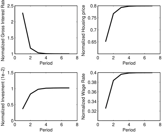
Figure 4: Transitional Dynamics after the Pension Reform

Model period equals 30 years. The fraction of homeowners ω = 0.33, payroll tax decreases to zero from τ = 0.40 after the reform, the downpayment ratio

dotted line denotes the demand and supply of loans before the pension reform. The

solid line denotes the loan demand and supply after the pension reform. Whether

the new equilibrium interest rate will be pushed down towards zero depends on

the tightness of collateral constraint. If the borrowing constraint is tight enough,

the increase in the loan supply will surpasses the increasing loan demand from

constrained homeowners. Therefore, bubble is possible.

Proposition 13 In the endowment economy, suppose the government remove the PAYG system. Bubble will arise if and only if θ > ω. A sufficient condition for housing wealth/GDP ratio to be higher than the pre-reform era isτ > θ−ω_1−ω.

Proof. See Appendix.

Figure 4 exhibits the policy experiments in all three cases, i.e.,θ < θL,θL <

θ < θH, and θ > θH. According to the Proposition 5, only pension reform in

case 2 and case 3 can trigger housing bubble.

In the production economy, the removal of pension system can trigger a

tran-sitional dynamics characterized by the following proposition.

Proposition 14 In the production economy, suppose the government remove the PAYG system and there exists a housing bubble in the new stationary equilibrium, then housing price and interest rate converge monotonically to the unique new steady state.

Proof. See Appendix.

During the transition, the housing price growth rate is equal to the gross

inter-est rate. The normalized interinter-est rate is defined as the gross interinter-est rate divided

by the gross population growth rate and productivity growth rate. The normalized

housing price growth rate is the housing price sequence divided by the current population and productivity. The investment is normalized in the similar way.

The normalized wage rate is defined as the wage rate divided by the current

3.2

Data

Housing price in China has been increasing strongly over the past decade. The

connected solid line in Figure 5 shows that the real land-selling price for the whole

country increases at an annual rate 15.7 percent from 2000 to 2009. There is no

constant quality official housing price index for China. I also draw the official

average commodity building selling price for 35 large cities in China. It shows a

slower annual growth rate, 7 percent, from year 2000 to 2009. Wu, Gyourko and

Deng (2012) also construct constant quality price index for newly-built private housing in 35 major Chinese cities. According to their estimate, the annual price

growth is nearly 10 percent from year 2000 to 2009. In the meantime, the US has

already experienced a burst in housing bubble in 2008.

The unprecedented housing boom in China encourage large increase real

es-tate investment and the boom in the home ownerships. As shown by Figure 6, the

share of real estate investment in total fixed investment increases from 13 percent

at 1999 to 20 percent at 2010. The urban households home ownerships rate

esti-mated from Urban Households Survey shows that China’s home ownership rate is

nearly 90 percent in 2010, among the highest in the world.3 These two facts

im-plies a lot of households own more than one apartment. Popular wisdoms claim that there is a housing bubble in China. One feature of the housing bubble is the

high vacancy rate in China. A vacant house/apartment is a unit that has been built

but is not occupied by anybody. The vacancy rate is defined as all vacant units/all

3_{The urban home ownership rate increases from less than 30 percent to 70 percent during}

4

4.5

5

5.5

6

Log Real Value

1990 1995 2000 2005 2010

date

Case−Shiller 10−MSA (US) Land Selling Price (China) Commodity Bldg Selling Price (China)

Figure 5: Housing Price and Land Price: China and the US

20

40

60

80

100

Homeownership Rate

.12

.14

.16

.18

.2

Share of Residential Investment

1990 1995 2000 2005 2010

year

Share of Residential Investment Homeownership Rate

Figure 6: Urban Residential Investment and Homeownership Rate

housing units (occupied + vacant). In the US, the gross vacancy rate is The gross

vacancy rates are 12.7, 13.0, 13.8, 14.4, 14.5, 14.3 during 2005-2010. In China,

according to the China Family Panel Studies 2011, 22 percent of urban

house-holds own more than one apartment. Only 25 percent of these rich househouse-holds

rent their apartments out. The vacancy rate in year 2010 is 11 percent according

to author’s estimate.

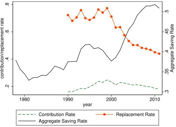
According to this paper, the insufficient social security for causing the

sky-rocketing housing prices because the elderly choose to own empty houses as a store of value to finance their later-life consumption. Figure 7 plots the pension

re-placement rate and contribution rate in China. The pension reform starts in China

from 1999, which changes the traditional pay-as-you-go (PAYG) system into a

mixture of PAYG system and fully-funded system. From then on, the replacement

rate of pension system decreases from around 75 percent to only 45 percent in

2009. During the same period, the saving rate in China increases by 15 percent,

which suggest that Chinese households increase savings partly to compensate the

huge decline in the pension payment.

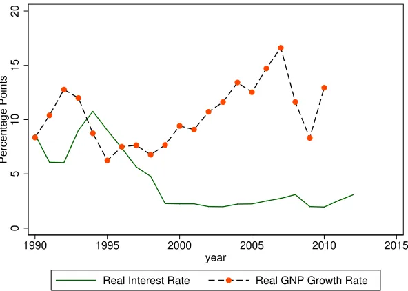
What if those households just invest their pension in terms of stocks and other

investment tools? Because the poor development in the financial market, the aver-age return on the stock market over the past twenty years in very low (the averaver-age

real return on shanghai stock market index is only 2 percent from year 2000 to

2009) and median households can only access to risk-free bond which delivers

almost zero interest actually. Therefore, the missing social security is

accompa-nied by the dynamic inefficiency in China. Figure 8 shows that the real interest

rate is China is much lower than the real growth rate, which makes risk-free bond

unattractive relative to housing investment for households.

Although there is studies documenting that the capital return in China is very high, however, those projects are not accessible to normal households in China.

In fact, Chinese government itself has accumulated great amount of foreign

as-sets and implicitly issue collateralized bonds to Chinese citizens. The low return

.3

.35

.4

.45

.5

Aggregate Saving Rate

.2

.4

.6

.8

contribution/replacement rate

1980 1990 2000 2010

year

Contribution Rate Replacement Rate Aggregate Saving Rate

Figure 7: Social Security Replacement Rate and Contribution Rate

0

5

10

15

20

Percentage Points

1990 1995 2000 2005 2010 2015

year

Real Interest Rate Real GNP Growth Rate

Figure 8: Dynamic Inefficiency

China. There are many reasons for causing the dynamic inefficiency problem,

e.g., the poor financial development, the absence of social security system, etc. If

the capital account were fully open, Chinese households would have purchased

huge amount of assets abroad directly. This dynamic inefficiency creates excess

supply of liquidity which allows for speculative bubble.

3.3

Test of the Model

The Chinese pension system is mainly operating at city or province level. Each

city or province has their own pension replacement standard and is running a

segmented pension fund account. Therefore, we can exploit the regional variation

in pension system to identify its effect on regional housing prices. If the theory

is correct, we would observe larger housing price appreciation for the province

where the pension contribution rate declines most. I first compute the theoretical

contribute rate τi,t_{, which is the tax rate that make the budget constraint of}

pay-as-you-go pension system holds for each provincei at yeart.

τi,t = expenditure

i,t

workeri,t ×wagei,t,i =1, . . . ,35,t =2001, . . . ,2011

where expenditurei,t the total expenditure of pension fund at provincei and year

t. workeri,t is the number of workered covered by the pension fund and wagei,t is the average wage rate of workers.

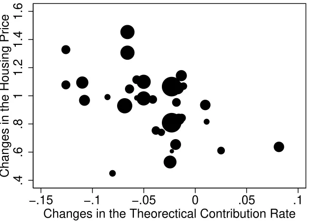
Figure 9 plots the changes in housing prices across 35 cities against the changes

in the theoretical contribution rates over year 2001-2011. There is a clear negative

correlation which confirms the prediction of the theory. The simple OLS univari-ate regression has a coefficient -2.84, which is significant at 1 percent confidence

level. The R squared is .24.

In order to estimate the effect of theoretical contribution rate on housing price

carefully, I estimate the following regression. However, the actual pension

contri-bution is usually higher than the theoretical contricontri-bution rate. I define the wealth

ac-.4

.6

.8

1

1.2

1.4

1.6

Changes in the Housing Price

−.15 −.1 −.05 0 .05 .1

Changes in the Theorectical Contribution Rate

Figure 9: Cross-section 10-year Changes in the Housing prices and Changes in the Theoretical Contribution Rate 2001-2011

Table 1: Regression Result on the Effect of Theoretical Contribution Rate on Housing Prices

Depend Var. log(housing price) Pooled regression Random Effect Fixed Effect

log(gdp) .0335 .157∗∗∗ .0335

(0.29) (3.61) (0.35)

Theoretical Contribution Rate -1.91∗∗∗ -1.88∗∗∗ -1.49∗∗∗

(-3.41) (-5.39) (-4.04)

Wealth Effect 1.42∗∗∗ 1.58∗∗∗ 1.42∗∗∗

(3.11) (4.12) (3.69)

Year Effect Yes Yes Yes

Province Dummies Yes Yes Yes

R-Squared 0.92 .68 .60

No. of Obs. 385 385 385

tual contribution rate. This measures the other channel which pension reform can

affect the households behavior and housing price.

ln Pi,t

=αZi,t +βτi,t +γwealth effecti,t

whereZi,tinclude the city dummies, year dummies and thelog gd pi,tfor province

i at yeart.

The result of regression is given by Table 1. The coefficient before the

the-oretical contribution rate is smaller than the slope in Figure 9. For example, the

fixed effect estimates shows that a 10 percentage points decline in the theoretical contribution rate contributed to a 14.2 percent increase in real housing price level.

4

Conclusion

This paper studies an economy inhabited by overlapping generations of

homeown-ers and investors, with the only difference between the two being that homeownhomeown-ers

derive utility from housing services whereas investors do not. Tight collateral

interest rate level down to the housing price growth rate, which makes housing

attractive as a store of value for investors. As long as the rental market friction is

high enough, the investors will hold a positive number of vacant houses in

equi-librium. A housing bubble arises in an equilibrium in which investors hold houses

for resale purposes only and without the expectation of receiving a dividend either

in terms of utility or rent. The model can be applied to China, where the housing

bubble can be attributed to the rapid decline in the replacement rate of the pension

system.

This paper also shed some lights on the issue of government debt. If the

gov-ernment lend to much if the borrowing constraint is high, it will only drive the

interest too low and investors will start to accumulate too much bubble asset. The

Chinese government has issued a rescue package after the financial crisis in the

US 2008, which triggered a further wave of housing price boom in China.

References

Arce, Aureo, and David Lopez-Salido. 2011. “Housing Bubbles.” American Economic Journal: Macroeconomics, 3(1): 212–41.

Brunnermeier, Markus K. 2009. “Bubbles: Entry in New Palgrave Dictionary of Economics.” , ed. Steven Durlauf and Lawrence Blume.

Caballero, Ricardo J., and Arvind Krishnamurthy.2006. “Bubbles and capital flow volatility: Causes and risk management.”Journal of Monetary Economics, 53(1): 35–53.

Caballero, Ricardo J., Emmanuel Farhi, and Pierre-Olivier Gourinchas.

2008. “An Equilibrium Model of &quot;Global Imbalances&quot; and Low

Interest Rates.”American Economic Review, 98(1): 358–93.

Farhi, Emmanuel, and Jean Tirole. 2012. “Bubbly liquidity.” The Review of Economic Studies, 79(2): 678–706.

Kocherlakota, Narayana. 2009. “Bursting bubbles: Consequences and cures.”

Unpublished manuscript, Federal Reserve Bank of Minneapolis.

Martin, Alberto, and Jaume Ventura.2012. “Economic Growth with Bubbles.”

American Economic Review, 102(6): 3033–58.

Miao, Jianjun, and Pengfei Wang. 2011. “Bubbles and Credit Constraints.”

Available at SSRN 1779485.

Samuelson, Paul A.1958. “An Exact Consumption-Loan Model of Interest with or without the Social Contrivance of Money.” Journal of Political Economy, 66: 467.

Tirole, Jean.1985. “Asset Bubbles and Overlapping Generations.”Econometrica, 53(6): 1499–1528.

A

Mathematical Appendix

A.1

Benchmark Model

A.1.1 Proof of Proposition 1

The Lagrangian function is

L =lnct_t +βlnc_tt₊₁

+λ1

(1−τ )y_tt −ct_t −a_tt₊₁− pthtt+1

+λ2

h

τ (1+n)y_tt₊+₁1+ Rt+1a_tt₊₁+ pt+1ht_t+1−c_tt₊₁

i

+µ₁a_tt₊₁+(1−θ)ptht_t+1

+ν1htt+1

The FOCs become

ct_t : 1

ct_t −λ1 =0

ct_t+1 : β

ct_t+1 −λ2 =0

a_tt₊₁ : −λ1+λ2Rt+1+µ1 =0

ht_t+1 : −λ1pt +λ2pt+1+µ1(1−θ ) pt+ν1=0

where

µ1 ≥ 0, ifatt+1+(1−θ)pthtt+1>0, thenµ1 =0

ν1 ≥ 0, ifh_tt+1 >0, thenν1=0

The life-time budget constraint for the investors is

c_tt + c

t t+1

Rt+1

=(1−τ )y_tt +τ (1+n)y

t+1

t+1

Rt+1

+

pt+1

Rt+1

− pt

1. a_tt₊₁+(1−θ )ptht_t+1 >0,i.e., the borrowing constraint of the investors is

not binding;ht_t+1>0,i.e., the unconstrained investors hold positive amount of housing. Thereforeµ1=ν1=0.Plug them into the FOCs

−λ1+λ2Rt+1 = 0

−λ1pt +λ2pt+1 = 0

The following equality holds

Rt+1 =

pt+1

pt

and the optimal consumption rules are

ct_t = 1

1+β

1−τ + τ (1+n) (1+g)

Rt+1

y_tt

ct_t+1 = βRt+1

1+β

1−τ + τ (1+n) (1+g)

Rt+1

y_tt

The allocation between the private IOUs and housing assets are

indetermi-nate. The total saving is determined by

at_t+1+pthtt+1=(1−τt)ytt −ctt

2. a_tt₊₁ + (1−θ ) ptht_t+1 > 0, i.e., the borrowing constraint of investor is

not binding; ht_t+1 = 0, i.e., the investor holds zero amount of housing. Therefore,µ1 =0, ν1≥0.Plug them into the FOCs,

−λ1+λ2Rt+1 = 0

−λ1pt +λ2pt+1+ν1 = 0

Hence,

Rt+1 ≥

pt+1

(a) Ifν1=0,then we go back to case 1

(b) Ifν1 >0,then Rt+1 > pt_p+_t1.The purchase of housing are less attrac-tive than the lending to the others.

a_tt₊₁ = (1−τ )y_tt −ct_t

ht_t+1 = 0

3. a_tt₊₁+(1−θ )ptht_t+1 =0,i.e., the borrowing constraint of the investors is binding; ht_t+1 > 0, i.e., the constrained investors hold positive amount of housing. Therefore,µ₁≥0, ν1 =0.

(a) Ifµ₁=v1=0,we go back to case 1. Ifµ1 >0, ν1=0, then

λ1

λ2

> Rt+1

λ1

λ2

> pt+1

pt

λ1

λ2

= pt+1−(1−θ )Rt+1pt θpt

Suppose pt+1

pt < Rt+1 <

λ1

λ2,then Rt+1 <

λ1

λ2 =

pt+1−(1−θ )Rt+1pt

θpt <

pt+1−(1−θ )pt+1

θpt =

pt+1

pt ,a contradiction! Therefore,

Rt+1<

pt+1

pt

< λ1 λ2

= pt+1−(1−θ )Rt+1pt θpt

Letγ_t ≡ λ1

λ2 =

pt+1−(1−θ )Rt+1pt

θpt .Rewrite the budget constraints as

c_tt = (1−τ )y_tt−θpthtt+1

Solve for ptht_t+1

pthtt+1 =

βγ_t(1−τ )−τ (1+n) (1+g) θ γ_t(1+β) y

t t

Therefore

c_tt = 1

1+β

1−τ +(1+n) (1+g) γ_t

y_tt

ct_t+1 = βγt

1+β

1−τ +(1+n) (1+g) γ_t

y_tt

at_t+1 = −(1−θ )ptht_t+1

pthtt+1 =

βγ_t(1−τ )−τ (1+n) (1+g) θ γ_t(1+β) y

t t

4. a_tt₊₁+(1−θ )ptht_t+1 = 0,i.e., the borrowing constraint of the investors is binding;ht_t+1=0,i.e., the investors hold positive amount of housing

c_tt = (1−τ )y_tt

ct_t+1 = τ (1+n) (1+g)y_tt

Thenµ₁, v1≥0.

−λ1+λ2Rt+1+µ1 = 0

−λ1pt +λ2pt+1+µ1(1−θ ) pt+ν1 = 0

(a) If µ₁, ν1 > 0, either investors have too little endowment when they

are young and do not want to save

λ1

λ2

> pt+1−Rt+1(1−θ )pt θpt

> pt+1

pt

or investors’ borrowing cost is too large

λ1

λ2

> Rt+1>

pt+1

pt

> pt+1−Rt+1(1−θ )pt θpt

In this article, I assume the young has enough endowment and wants

to save. Therefore, I rule out the case λ1

λ2 >

pt+1−Rt+1(1−θ )pt

θpt >

pt+1

pt >

Rt+1.

(b) Ifµ1>0, v1=0,We go back to Case 3

(c) Ifµ₁=0, ν1 >0,We go back to Case 2

(d) Ifµ₁=0, v1=0,We go back to Case 1

A.1.2 Proof of Proposition 2

The Lagrangian function is

L =lnct_t +βζln ht_t+1+β (1−ζ )lnct_t+1

+λ1

(1−τ )yt − ptht_t+1−c

t

t −att+1

+λ2

τ (1+n) (1+g)yt +Rt+1att+1+ pt+1htt+1−ctt+1

+µ₁a_tt₊₁+(1−θ)ptht_t+1

The FOCs become

c_tt : 1

ct_t −λ1 =0

c_tt₊₁ : β (1−ζ )

ct_t+1 −λ2 =0 a_tt₊₁ : −λ1+λ2Rt+1+µ1 =0

ht_t+1 : βζ

where

µ₁ ≥0, ifa_tt₊₁+(1−θ ) ptht_t+1>0, thenµ1=0

and the life-time budget constraint is given by

c_tt + c

t t+1

Rt+1

+

pt−

pt+1

Rt+1

ht_t+1=(1−τ )y_tt+ τ (1+n)y

t+1

t+1

Rt+1

1. a_tt₊₁+(1−θ )ptht_t+1 >0,i.e., the borrowing constraint of the homeowners

is not binding. Therefore,µ₁=0.Hence,

λ1

λ2

= Rt+1=

pt+1+ _1−ζζ

ct_t+1 ht_t+1

pt

The optimal decision rules are

c_tt = 1

1+β

1−τ + τ (1+n) (1+g)

Rt+1

y_tt

ct_t+1 = β (1−ζ )Rt+1

1+β

1−τ +τ (1+n) (1+g)

Rt+1

y_tt

pthtt+1 =

1 1− pt+1

ptRt+1

βζ

1+β

1−τ + τ (1+n) (1+g)

Rt+1

y_tt

a_tt₊₁ = (1−τ )y_tt− ptht_t+1−c

t t

2. a_tt₊₁+(1−θ )ptht_t+1 =0,i.e., the borrowing constraint of the homeowners is binding. Therefore,µ1 ≥0

(b) Ifµ₁>0

−λ1+λ2Rt+1+µ1 = 0

βζ

ht_t+1 −λ1pt +λ2pt+1+µ1(1−θ )pt = 0

Hence, the condition for Rt+1is given by

Rt+1<

λ1

λ2

Let λ1

λ2 ≡γt,then from the budget constraint

ct_t =(1−τ )y_tt −θpthtt+1

and

c_tt₊₁=τ (1+n) (1+g)y_tt +(pt+1−Rt+1(1−θ )pt)htt+1

From the FOC w.r.t.ht_t+1,we have

βζ

ht_t+1 −λ1θpt +λ2(pt+1−Rt+1(1−θ )pt)=0

Use the expression forλ1, λ2,we have

1 = λ1(1−τ )ytt −λ1θptht_t+1

β (1−ζ ) = λ2τ (1+n) (1+g)y_tt +λ2(pt+1−Rt+1(1−θ )pt)ht_t+1

βζ = λ1θpthtt+1−λ2(pt+1−Rt+1(1−θ )pt)htt+1

Therefore

Note that

1+β = (1−τ )y

t t

(1−τ )y_tt −θptht_t+1

+β (1−ζ ) τ (1+n) (1+g)y

t t

τ (1+n) (1+g)y_tt+(pt+1−Rt+1(1−θ )pt)ht_t+1

This is a quadratic equation for ptht_t+1.Let

x = ptht_t+1

ϕ = pt+1

pt

−(1−θ )Rt+1

a = (1−τ )y_tt

b = τ (1+n) (1+g)y_tt

Then

1+β = a

a−θx +

β (1−ζ )b b+ϕx

It has a unique positive solution

ptht_t+1 =x =

9t +8t

2θϕ (1+β)

where 9t = aϕβ − bθ (1+βζ ) , 8t =

q

9_t2+4abθβζ ϕ (β+1).

We can defineγ_t

γ_t = λ1 λ2

= c

t t+1

β (1−ζ )ct_t =

b+ϕx

and

c_tt = 1

1+β

1−τ + τ (1+n) (1+g) γ_t

y_tt

c_tt₊₁ = β (1−ζ ) γt

1+β

1−τ + τ (1+n) (1+g) γ_t

y_tt

pthtt+1 =

βγ_t(1−τ )−τ (1+n) (1+g) θ γ_t(1+β) y

t t

A.1.3 Proof of Lemma 1

We start first by looking the saving function of the unconstrained homeowner/investor.

It is obvious to see the saving function of the unconstrained homeowner/investor is

a decreasing function of interest rate. When the investor is borrowing constrained,

higher interest rate reduces γ_t and implies fewer housing bought. Hence, the

amount investor can borrowing is a decreasing function of interest rate. When the

homeowner is borrowing constrained, the loan demand function becomes

compli-cated. Differentiate ptht_t+1directly w.r.t.ϕ

ptht_t+1 =

9t+

q

9_t2+4abβζ θϕ (β+1)

2θ ϕ (β+1)

= 4abβζ θϕ (β+1)

2θ ϕ (β+1)

q

9_t2+4abβζ θ ϕ (β+1)−9t

= 2abβζ_q 1

Then

∂ptht_t+1

∂ϕ = −2abβζ

 

1

q

9_t2+4abβζ θ ϕ (β+1)−9t

 

2

×

d dϕ

q

9_t2+4abβζ θ ϕ (β+1)− d

dϕ9t

Note that9t =aϕβ−bθ (1+βζ )

d

dϕ9t =aβ

and also

d dϕ

q

9_t2+4abθ βζ ϕ (β+1)

= _qaβ9t +2abβζ θ (β+1) 9t2+4abβζ θϕ (β+1)

= aβ(aϕβq−bθ (1+βζ ))+2bζ θ (β+1)

9_t2+4abβζ θ ϕ (β +1) < aβ

because

((aϕβ−bθ (1+βζ ))+2bζ θ (β+1))2−9_t2+4abβζ θ ϕ (β+1)

= −4b2ζ θ2(β+1) (1−ζ ) <0

Therefore,

∂ptht_t+1

∂ϕ >0,

∂ptht_t+1

∂R <0

The loan demand of constrained homeowner is an increasing function of interest