Munich Personal RePEc Archive
Implementation Issues in the
Duclos-Jalbert-Araar Decomposition of
Redistributive Effect
Ivica, Urban
Institute of Public Finance
11 January 2011
Online at
https://mpra.ub.uni-muenchen.de/58826/
1
The Duclos-Jalbert-Araar Decomposition of Redistributive
Effect: Implementation Issues
IVICA URBAN
Institute of Public Finance, Zagreb, Croatia, [email protected]
Version: May 5, 2012
Abstract
Models decomposing the redistributive effect of fiscal systems into vertical and horizontal effects
are extensively used by practitioners. The Duclos, Jalbert, and Araar’s (2003) model, despite its
advantages, has not yet been widely employed in empirical research, possibly due to a relatively
challenging implementation procedure that involves the estimation of expected post-fiscal incomes.
To override these difficulties the designers of the software DAD (Duclos, Araar, and Fortin 2010)
have incorporated a module for implementation of the model. However, the application of this
module on Croatian tax-benefit system data revealed certain inaccuracies in the results. Carefully
unfolding the calculation and estimation procedures needed for implementation of the model, this
paper instructs practitioners on how to correctly apply the model and helps DAD designers improve
their module.
Keywords: redistributive effect, vertical equity, horizontal inequity, pre-fiscal equals
2
1 INTRODUCTION
Duclos, Jalbert, and Araar (2003) (henceforth DJA) have designed a comprehensive model to
decompose the redistributive effect (RE) of a fiscal system into vertical, classical horizontal inequity
(henceforth CHI), and reranking effects. The model is built into the framework of the Atkinson-Gini
social welfare function (henceforth AGF), which first converts incomes into utilities employing the
Atkinson’s (1970) utility function, and then aggregates utilities using rank-dependent weights,
which underlie the S-Gini and S-concentration coefficients proposed by Donaldson and Weymark
(1980) and Yitzhaki (1983).1
The DJA model has certain advantages over its competitors, the widely acknowledged
Kakwani’s (1984) (henceforth K84) and the Aronson, Johnson, and Lambert’s (1994) (henceforth
AJL) decompositions of RE. To measure the CHI effect, the researcher must determine the set of
counterfactual CHI-free or expected post-fiscal incomes (EPIs). While the AJL model relies on the
formation of arbitrary groups of close equals in this task, the DJA model employs purposefully
designed statistical procedures. Consequently, the implementation of the DJA model requires a
certain expertise related to data smoothing and curve-fitting methods. To facilitate the application
of the DJA model in empirical analysis, a module for calculation of the DJA indices from the sample
data is incorporated into the software DAD (Duclos, Araar, and Fortin 2010) (henceforth DAD-DJA).
The use of DAD-DJA in research on the Croatian tax-benefit system revealed certain
inaccuracies in the results. Specifically, when the ethical parameter of AGF is set to zero, the CHI
effect in the DJA model should be equal to zero by construction. However, the estimated value of the
CHI effect was significantly different from zero. Analysis has shown that DAD-DJA produces upward
biased estimates of EPIs in the low pre-fiscal income region. Furthermore, it was revealed that the
fitting procedure in DAD-DJA contains a ‘bug’, producing unreasonably high estimates of EPIs for the
3
In an attempt to obtain fully accurate estimates of DJA indices, independent procedures have
been developed. They are thoroughly explained in this paper to assist practitioners in implementing
the DJA model and to help DAD designers improve the working of DAD-DJA. A brief overview of data
smoothing methods is provided, accompanied by advice on how to accurately obtain EPIs estimates.
Relationships with other measurement models are explained.
The rest of the paper is organized as follows. Section 2 briefly exposes the elements of the
DJA model and its connections with other decompositions. Section 3 extensively describes the
procedures of data preparation, estimation and calculation of various elements of the DJA model,
and employs them on a simple hypothetical population of four income units. In section 4 the
procedures are applied to data on the Croatian tax-benefit system, and the results are compared
with those obtained by DAD-DJA. Section 5 concludes the paper.
2 THE DUCLOS-JALBERT-ARAAR MODEL
Post-fiscal income is equal to pre-fiscal income minus taxes plus benefits. The change of income
inequality induced by a fiscal system consisting of taxes and benefits is called the redistributive
effect (RE). In measurement terms, we have that ∆ , where ∆ represents RE, and
and are indices of pre- and post-fiscal income inequality.
In the DJA model, inequality indices · are derived using the Atkinson-Gini social welfare
function, proposed by Araar and Duclos (2003, 2006). For pre-fiscal income we have that
, ,ν , ,ν 1
where is the ethical parameter configuring the Atkinson’s (1970) utility function, ,
/ 1 for 1, and , ln for 1, with denoting the quantiles of
the pre-fiscal income distribution, and the income at quantile . The term ν is another ethical
parameter, characterizing the Donaldson and Weymark’s (1980) and Yitzhaki’s (1983) S-Gini
4
an inverse function of · and is obtained as ξ , ,ν 1 , ,ν / for 1, and
ξ , ,ν exp , ,ν for 1. Finally, the Atkinson-Gini inequality index is calculated as
follows:
1 ξ , ,ν /!" (2)
where !" is the mean pre-fiscal income. is obtained analogously, using the quantiles of the
post-fiscal income distribution.
The DJA model decomposes RE as follows:
∆ # $ % & ' & ' (3)
The vertical effect, # & , represents the potential RE or the reduction of
inequality that would be achieved by the counterfactual, CHI-free system. The discrepancy between
potential and actual RE is divided into a CHI effect, $ ' & , and a reranking effect,
% ' , which measure two different manifestations of horizontal inequity (HI). The
former effect (C) measures HI emerging from violation of the ‘classical horizontal equity principle’,
which says that equals should be treated equally. The latter effect (R) evaluates HI arising from
infringement of the ‘no-reranking principle’, which requires the fiscal process to not change the
ranks of income units in transition from pre- to post-fiscal income. Take, for example, four
households of equal size. A and B have fiscal incomes of 10 each, whereas C and D have
pre-fiscal incomes of 20 each. Suppose that A, B, C, and D end up with post-pre-fiscal incomes of 8, 16, 12,
and 24, respectively. Between pre-fiscal equals (A and B; C and D) CHI has occurred, whereas
between pre-fiscal unequals (B and C) reranking has taken place.
In equation (3), & is the inequality index obtained for EPIs, equal to &
(| (, where (| denotes a post-fiscal income at the qth quantile among all those income
5
inequality index obtained for expected post-fiscal utilities (EPUs) at quantile p, ' ,
(| , (. For & and ' , we obtain the respective social welfare functions
&, ,ν & , ,ν and ', ,ν ' , ,ν , while the
corresponding inequality indices are & 1 ξ &, ,ν /!* and ' 1 ξ ', ,ν /!*,
where !* is the mean post-fiscal income.
In the special case where 0, utilities are identical to incomes: :, 0 :. Therefore, we
have that (| , (| across all p and (| , and it follows that &, 0,ν
', 0,ν and &, 0,ν ', 0,ν . The consequence for the DJA model is that the CHI effect
collapses to zero, and the decomposition 3 can be rewritten as
∆ 0,ν # 0,ν % 0,ν , 0,ν &, 0,ν , 0,ν &, 0,ν (4)
It can be shown that , 0,ν , , 0,ν , and &, 0,ν are the S-Gini coefficient of pre-fiscal
income, H ,ν , the S-Gini coefficient of post-fiscal income, H ,ν , and the S-concentration
coefficient of post-fiscal income, I ,ν , respectively.2
Consequently, # 0,ν is equal to the S-Gini Kakwani’s (1984) index of vertical effect,
#J ν H ,ν I ,ν , and % 0,ν is the S-Gini Atkinson (1980), Plotnick (1981), and
Kakwani’s (1984) index of reranking, %K'J ν H ,ν I ,ν . The Kakwani’s (1984)
decomposition of RE into vertical and horizontal components can be rewritten in S-Gini terms as
∆ ν #J ν %K'J ν H ,ν I ,ν H ,ν I ,ν (5)
In another special case, where ν 1, the weights ,ν are equal for all p and the
reranking effect disappears. For L 0, the vertical and CHI effect, # , 1 and $ , 1 , become the
6
3 CALCULATION OF INDICES
3.1. Data Preparation
A typical research uses the following data for a household or family i: (a) unequivalized pre- and
post-fiscal incomes, MN and MN; (b) survey frequency (or sampling) weights, ON; and (c) equivalence
factor PN. The equivalized pre- and post-fiscal incomes are N MN/PN and N MN/PN (hereafter we
deal only with equivalized incomes, calling them plainly pre- and post-fiscal incomes). The
frequency weights are defined as φN ONPN. Thus, the equivalence factor PN is employed both for
deriving the equivalized income and for weighting households of different types.4
We form the 3 Q R matrix S , where R is the number of households in the sample:
S T …… NN … … VV φ … φN … φVW
(6)
To obtain the matrix SX (SY), the columns in S are sorted in increasing order of the values from the first (second) row:
SX T
X …
NX … VX X …
NX … VX φX … φNX … φVX
W; SY T
Y …
NY … VY Y …
NY … VY φY … φNY … φVY
W (7)
From SX we take out the values NX, NX, and φXN, while from SY the values NY and φNY. and
are extracted. Notice that the superscript x (n) denotes that income units are sorted in increasing
order of pre-fiscal (post-fiscal) income.
The sample estimates of quantiles p and the weights ,ν are obtained in the following manner:
ZNX 2Σ ∑ ]φ
^X_φ^X ` N
^a
bNX,ν Σ ν 1 Z
7 where Σ ∑V^a φ^X and φX 0.
When a large group of pre-fiscal exact equals exists in the sample, one of the inequality
indices would be biased if based on the weights bNX,ν, namely, cd
NX, ,ν; bNX,νf from equation (17) (see later discussion). Therefore, we derive a new set of weights, ωgNX,ν. Assume that income units
h 1, … , i have zero pre-fiscal incomes, i.e., X jX k lX 0, and corresponding post-fiscal
incomes X, jX, … , lX. The procedure described by equation (8) automatically ascribes to these
units the weights that are strictly decreasing in i and ZNX, i.e., bX,νL k L blX,ν, although all these
units have equal pre-fiscal income and rank. Therefore, we replace them with the new set of weights
obtained as follows:
ωgNX,ν d∑lma φmXf ∑nal φnX· bnX,ν, for h 1, … , i
ωgNX,ν bNX,ν, for h L i (9)
Thus, the original weights bNX,ν of pre-fiscal equals are transformed into their group average. An analogous procedure should be applied to other large groups of pre-fiscal equals, if they exist in
the sample.
Alternatively, we could use the original weights and randomize the order of income units
within each group of exact pre-fiscal equals. This procedure would reduce the bias to an
insignificant level, but each possible ordering of income units would still result in different values of
cd NX, ,ν; bNX,νf. However, for purposes of consistency and transparency, the use of weights ωgNX,ν is
recommended. For all the other indices derived below, it is irrelevant whether the weights bNX,ν or
ωgNX,ν are employed, because the income vectors they are based upon (namely, NX, N,', and N&) have identical values within a group of exact pre-fiscal equals.
Finally, analogously to the above procedures, the estimates ωgNY,ν are obtained from φNY (for
8
3.2 Indices of Inequality
The following equations show how to obtain utilities, the Gini-Atkinson welfare index, and the
inequality index for pre-fiscal incomes NX, when 1:
NX, NX / 1 o d NX, ,ν;ωg
N
X,νf ∑ d
^X, f ·φ^X·ωg^X,ν V
^a
pd NX, ,ν;ωgNX,νf 1 q 1 o d NX, ,ν;ωgNX,νfr
s
stu/!̂ NX (10)
where !̂ NX Σ ∑V^a φ^X· ^X is the mean pre-fiscal income. To shorten the presentation, the
formulas referring to the case where 1 are omitted. Analogously, the utilities and indices for
post-fiscal incomes NY are obtained, as shown by equation (16) in the Appendix.
pd NX, ,ν;ωg
NX,νf and pd NY, ,ν;ωgNY,νf from (10) and (16) are the sample estimates of the indices of pre- and post-fiscal income inequality, and . As equation (3) indicates, the
application of the DJA model requires the estimates of two other indices, & and ' , derived
from EPIs, & , and EPUs, ' , .
To obtain the sample estimates of EPUs, N,', we should smooth a dataset
w NX, NX, ;φNXxNaV . For each value of ε, we estimate the regression relationship NX,
y',
NX _ zN, to obtain the approximation y{', · . Subsequently, the vector of fitted values is
calculated as N,' y{', NX .
However, the following identity says that the whole procedure of estimating EPUs can be
circumvented, saving the practitioner’s time and energy in sensitivity analysis using multiple
scenarios for ν and . Genuinely, the sample estimate of ' is equal to pd N,', ,ν;ωgNX,νf from
equation (20), but it can be derived more simply by the inequality index pd NX, ,ν;ωgNX,νf from
equation (18), because of the following equality:
9
To understand why (11) holds, recall that ' , (| , ( and notice that the
theoretical values (| are represented by the sample values X. Imagine the population
consisting of two groups of exact pre-fiscal equals: B income units have pre-fiscal income X and
post-fiscal incomes X, … , |X, while F income units have pre-fiscal income Xj L X and
post-fiscal incomes |}X , … , |}~X . Their rank-dependent weights are ωgX,ν k ωg|X,ν ωgX,ν and
ωg|}X,ν k ωg|}~X,ν ωgX,jν. For given , the values of expected post-fiscal utilities, N,', are obtained
as averages of utilities ' , • ∑|^a d ^X, f and 'j , € ∑|}~^a|} d ^X, f. The welfare is
then obtained by (20) as
o d N,', ,ν;ωgNX,νf • ·ωgX,ν· • • d ^X, f |
^a _ € ·ωg j
X,ν
· € •|}~ d ^X, f
^a|}
ωgX,ν· •| d ^X, f
^a _ωg j
X,ν
· • d ^X, f
|}~
^a|}
Observe that according to (18) we would obtain the identical result for o d NY, ,ν;ωgNY,νf.
Consequently, pd N,', ,ν;ωgNX,νf and pd NX, ,ν;ωgNX,νf are also identical.
3.3 Estimation of Expected Post-fiscal Incomes and Utilities
Unlike the estimation of EPUs, the evaluation of EPIs cannot be avoided. To obtain the sample
estimates of & , we must smooth a dataset w NX, NX;φNXx
Na V
, i.e., approximate the mean response
curve y& in the regression relationship NX y& NX _ ‚N. The estimates of EPIs are then obtained
as N& y{& NX , where y{& NX is the approximation of y&.
The estimation of EPIs represents the greatest challenge in the implementation of the DJA
model. Although parametric models (such as polynomial regression) can be appropriate for some
datasets, it is better to rely on non-parametric approaches, assuming no a priori functional
relationship between post- and pre-fiscal incomes. One such approach is the ‘kernel-weighted local
10
(1996), Wand and Jones (1995), Keele (2008), and Härdle (1990), while the software applications
include Stata 12 (function lcpoly), R (function loess, package lokern, etc.), and XploRe (function
lpregxest).
The choice of the degree of polynomial (p), the type of the kernel function, and the size of the
kernel half-bandwidth rests on the analyst. For 0, KWLPR becomes the ‘Nadaraya-Watson
estimator’ (NWE), while for 1 we obtain the ‘local linear estimator’ (LLE). Fan and Gijbels
(1996) explain that the odd degree polynomials achieve the best balance between bias and
variability and automatically correct the boundary problem.
Another interesting smoothing technique came to light during the research: the ‘Fourier
series in trigonometric form’ (FSTF), which is a sum of sine and cosine functions describing a
periodic signal (Faunt and Johnson 1992). The estimation procedure is programmed in Matlab
R2011b’s Curve Fitting Toolbox 3.2, which contains several other fitting methods, such as
smoothing splines.
DAD-DJA and supporting documentation5 do not inform us which fitting method is used to
obtain EPIs for estimation of DJA indices. However, DAD incorporates a separate module, ‘Non
Parametric Regression’, enabling us to estimate EPIs independently of DAD-DJA. Two basic methods
are offered: NWE and LLE (henceforth DAD-NWE and DAD-LLE). Experimentation with different
options and choices offered by the module revealed that in estimating EPIs DAD-DJA in fact employs
DAD-LLE, using the default set of parameters.
Before moving further, we offer the following advice to help judge whether the estimates N&
are appropriate for use in the DJA model implementation.
(a) Although the fitting methods and their software implementations ensure optimality in the
statistical sense, the analyst still has the freedom and the responsibility to change some of the
parameters or the whole estimation method if the results contradict her/his knowledge of the
11
‘stretch’ it, perhaps by raising the kernel half-bandwidth. Another example may be the existence of
certain kinks or local minimums (maximums) we are aware of, which are not reflected by the EPIs
estimate.
(b) For certain data points the programmed fitting procedures may produce irregular results.
Some software tools are ‘smart’ in such cases, leaving a blank space instead of the estimate, while
others are not. Anyway, if this happens we should fill in the corresponding estimate manually, using
the best-guess approach.
(c) A simple preliminary test of the correctness of the approximation y{& NX is to check
whether the mean value of the estimated values N& is approximately equal to the mean of the
sample values NX, i.e., if
!̂d N&f !̂
NX (12)
(d) The discussion in section 2 indicated that when 0, we have that NX, 0 NX, and
N,' N&. Therefore, equation (11) becomes
pd N&, 0,ν;ωgNX,νf pd N,', 0,ν;ωgNX,νf pd NX, 0,ν;ωgNX,νf (13)
From equation (13) follows another test: the inequality indices pd N&, 0,ν;ωgNX,νf, obtained by
equation (19), for different values of parameter ν should be (approximately) equal to the inequality
indices obtained for pd NX, 0,ν;ωgNX,νf. Otherwise, the estimates of the DJA indices would be biased,
and we should try to obtain an alternative configuration of y{& NX .
3.4 Decompositions
Having defined all the indices needed, we can present RE and its decompositions in terms of sample
estimate formulas. RE is obtained as ∆ƒ p NX p NY . According to the DJA model from (3), RE is
decomposed as follows:
12
q p NX pd N&fr qpd N,'f pd N&fr q p NY pd N,'fr
q p NX pd N&fr qp NX pd N&fr q p NY p NX r (14)
where the last row in equation (14) arrives from the property (11), by which pd N,'f p NX . The
differences in the brackets, i.e., #ƒ p NX pd N&f, $p pd N,'f pd N&f p NX pd N&f, and
%ƒ p NY pd N,'f p NY p NX , are respectively the sample estimates of the vertical, CHI, and
reranking effects of the DJA model. Note that, if c NX is used instead of p NX , the CHI and
reranking effects would be biased. Furthermore, if the estimates N& are inappropriate, the vertical
and CHI effect would be biased.
Setting 0 and following (4) and (5), we can calculate the S-Gini K84 decomposition as
∆ƒ #„J ν %…K'J ν
q pd NX, 0,ν;ωg
NX,νf pd NX, 0,ν;ωgNX,νfr q pd NY, 0,ν;ωgNY,νf pd NX, 0,ν;ωgNX,νfr (15)
3.5 Simple Hypothetical Example
We return to the example of four hypothetical households from section 2 to illustrate how the DJA
model implementation procedures work. There are two groups of pre-fiscal equals in the sample: A
and B with fiscal income of 10 each belong to the lower quantile, whereas C and D with
pre-fiscal income of 20 each belong to the upper quantile of pre-pre-fiscal income distribution.
The first column in Table 1 shows the ‘original’ weights bNX,ν obtained by (8) for ν 2;
observe that A (C) obtains larger weight than B (D), although they belong to same pre-fiscal
quantile. Therefore, analogously to the procedure from equation (9), we obtain the new set of
weights, ωgNX,ν: for A and B (C and D) we have ωgX ωgjX bX_ bXj /2 [ωg†X ωg‡X b†X_ b‡X /2].
Table 1
As equation (11) explains, the estimate of ' can be obtained in two ways: by pd N,'f or
by p NX . In the former case, we first obtain the values N,', which are the sample estimates of
13
X and jX ( †X and ‡X), and the corresponding utilities are X and jX [ †X and ‡X ].
The expected post-fiscal utility at each quantile is simply the average utility of units belonging to the
corresponding quantile: ' j' X _ jX /2 and †' ‡' †X _ ‡X /2, for
the lower and the upper quantiles, respectively.
According to (20), for ν 2 and 0.5 we have that
o d N,', ,ν;ωg
NX,νf 2 · '·ωgX_ 2 · †'·ωg†X 7.21
and pd N,', ,ν;ωgNX,νf 0.133. Substituting back previously obtained utility terms into the expression
for welfare, we obtain
o d N,', ,ν;ωgNX,νf X _ jX ·ωgX_ †X _ ‡X ·ωg†X 7.21
which is identical to the result that would be obtained by (18):
o d NX, ,ν;ωgNX,νf X ·ωgX_ jX ·ωgjX_ †X ·ωgX†_ ‡X ·ωg‡X 7.21,
Thus, our hypothetical example confirms the identity (11). On the other hand, indices based
on the ‘wrong’ weights, bNX,ν, would produce quite a different picture. By (17) we have
Š d NX, ,ν; b
NX,νf X · bX_ jX · bjX_ †X · b†X_ ‡X · b‡X 6.89,
and cd NX, ,ν; bNX,νf 0.210.
The estimate of & is obtained as pd N&, ,ν;ωgNX,νf from (19), which is in turn based on
sample estimates N& of & (| (. In this example we can simply calculate & j&
X_
jX /2 and †& ‡& †X_ ‡X /2. According to (19),
o d N&, ,ν;ωgNX,νf 2 · &·ωgX_ 2 · †&·ωg†X 7.32,
14
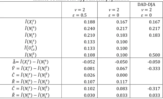
All inequality indices for ν 2 and 0.5 are presented in the first column of Table 2,
together with the DJA decomposition results. Although the vertical effect of the hypothetical system
is positive (#ƒ 0.081), the redistributive effect is negative (∆ƒ 0.052), because the CHI effect
($p 0.026) and especially the reranking effect (%ƒ 0.107) are very large.
Table 2
Another set of CHI and reranking effects is derived using c NX , which is based on the
weights bNX,ν. They show a completely different picture of the relative contributions of CHI
($c 0.102 vs. $p 0.026) and reranking (%Ž 0.030 vs. %ƒ 0.107) to the overall HI. We have
indicated that the weights ωgNX,ν are the ‘right ones’, but to demonstrate this in our example, we have to obtain the indices for ν 2 and 0, shown in the second column of Table 2.
Recall that equation (13) says that the inequality indices based on NX, N,', and N& must be
equal when 0; this is true for p NX 0.100, but not for c NX 0.183. The difference
c NX p
NX 0.083 presents by how much the CHI effect, which should be zero when 0, is
overestimated if the weights bNX,ν are used in computation of the inequality index for post-fiscal
incomes NX.
Finally, we look at how DAD-DJA deals with this small hypothetical case. The DAD
supporting documentation tells us that the estimate of ' is obtained by the index based on NX;
its value for ν 2 and 0 (0.183) is identical to c NX . This indicates that DAD-DJA does not
envisage the presence of exact equals in the sample. The third column in Table 2 shows the other
results. The index pd N&f diverges highly from our estimate (0.500 vs. 0.100), but this may be due to
15
4 APPLICATION: CROATIAN TAX-BENEFIT SYSTEM
4.1 Data
We analyze the fiscal system consisting of social security contributions (SSC) for the pension, health,
and unemployment insurance funds, personal income tax and surtax (PITS), public pensions, and
cash social benefits.6 The data on incomes come from the Croatian household budget survey (Anketa
o potrošnji kućanstava; APK) for 2008, whose sample contains 3,108 households. Since APK
registers only net incomes of household members, the amounts of pre-fiscal income, PITS, and SSC
are obtained by a microsimulation model.
Post-fiscal income of a household i is obtained as MN MN •MN_ •MN, where MN, •MN, and •MN are
pre-fiscal income, the sum of all taxes paid, and the sum of all benefits received. To obtain N and N,
MN and MN are deflated by the equivalence factor PN according to the ‘modified OECD scale’,
PN 1 _ 0.5 •N 1 _ 0.3‘N, where •N and ‘N are numbers of adults and children in household i.
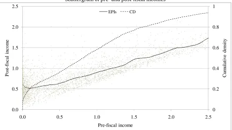
Before analyzing the results of the DJA decomposition, we observe the features of the data
set. The dots in the scattergram (Figure 1) are the post-fiscal and pre-fiscal incomes of sample
income units, expressed in terms of the mean pre-fiscal income (mpfi). The full line shows EPIs
obtained by KWLPR (see next section for details on estimation). The dotted line represents the
cumulative density, which tells us, for each pre-fiscal income X, the proportion of all income units
having pre-fiscal income below X (on the right axis). We can observe that quite a large proportion of
units, about 7 percent, have zero pre-fiscal income (group A), while the next 13 percent of units
have pre-fiscal income below 10 percent of mpfi (group B).
Figure 1
The mean post-fiscal incomes of groups A and B are 64 and 54 percent of mpfi, respectively.
Observe that the EPIs curve is decreasing on the interval [0, 0.1]. The following three facts taken
16
majority of pensioners’ households a public pension is the only source of income; since public
pensions are benefits in the current scenario, the pre-fiscal income of most pensioners’ households
is zero. Second, majority of households with zero pre-fiscal income (group A) are pensioners’
households. Third, pensions are on average higher than other social benefits.
4.2 Estimation of Expected Post-fiscal Incomes and the Decomposition
The indices of the DJA decomposition are estimated by three models, using three different fitting
methods described in section 3.3.
In model A, EPIs are estimated by KWLPR programmed in Stata 12. Following Bilger (2008),
we use the 3rd degree local polynomials, employing the Epanechnikov kernel. The optimal
half-bandwidth of the kernel obtained by the program was equal to 6.7 percent of mpfi and it was
increased by one half. In model B, EPIs are obtained using FSTF programmed in Matlab R2011b’s
Curve Fitting Toolbox 3.2. The number of harmonics is set to 7; the “Trust-Region” algorithm is
employed with the robust fitting option turned off. In both models the top five pre-fiscal income
units are excluded from the fitting process, and their values of N& are set to the values of NX. The
size of the half-bandwidth in model A and the number of harmonics in model B are chosen to
minimize the bias pd NX, 0,ν;ωgNX,νf pd N&, 0,ν;ωgNX,νf. For the estimates of ' , we used
pd NX, ,ν;ωgNX,νf with weights ωgNX,ν obtained by equation (9).
The aim of model C is to replicate the results obtained by DAD-DJA. We employ DAD-LLE to
estimate EPIs, with all observations included in the fitting process. To estimate ' , DAD-DJA also
uses the index based on NX, but does not envisage the possibility of pre-fiscal exact equals. To play
down the bias in the calculation of reranking and CHI effects, we randomize the order of income
units within the group of zero pre-fiscal equals; these data are then put into DAD-DJA to obtain the
17
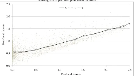
Before moving on to the results, let us look at the shapes of the different EPIs curves, shown
in Figure 2, concentrating first on the bottom part of the income distribution. While A and B both
reflect the initial fall in expected post-fiscal income, discussed above, C does not, i.e., its EPIs curve is
rather flat on the whole interval. For pre-fiscal income of zero all estimates are roughly the same,
but in the pre-fiscal income interval [0.025, 0.42] of mpfi, C’s EPIs lie above those estimated by A
and B. On the pre-fiscal income interval [0, 0.5] of mpfi the mean of EPIs obtained by A (B) is 0.5764
(0.5775) of mpfi, which is very close to the mean post-fiscal income for actual values, equal to
0.5762. On the other hand, the mean of EPIs obtained by C is 0.5881, or 2 percent above the actual
mean. This suggests that C overestimates EPIs for the lowest incomes. For pre-fiscal incomes above
0.5 of mpfi, the EPIs of B and C are almost identical, while the EPIs curve of A is “more flexible” and
intertwining the other two curves.
Figure 2
Models A and B convincingly pass the test from equation (12), as the ratios !̂d N&f/!̂ NX in
Table 3 are 0.999732 and 1.0, respectively. On the other hand, for method C, !̂d N&f is 1.75 percent
higher than !̂ NX . This is partly the consequence of the earlier noticed overestimation on the
interval [0, 0.5] of mpfi. However, there is another feature that is particularly odd: the estimate N&
for the two income units with top pre-fiscal incomes are 2.4 and 6.4 times larger than their
respective actual post-fiscal incomes NX! In this case we can talk about a ‘bug’ in DJA-LLE, which
seriously damages the estimate of !̂d N&f, which will lead to biased estimates of vertical and CHI
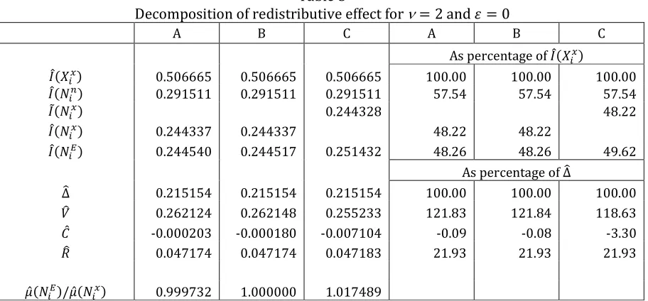
effects, as we will soon observe. Table 3 shows the results of the DJA decomposition for ν 2 and
0. All three models obtain equal values of p NX and p NY . Models A and B obtain the value of p NX equal to 0.244337, which is almost insignificantly different from the value of c
NX obtained
by model C, thanks to randomizing the order of income units within the group of zero pre-fiscal
18
(or decreasing) order of post-fiscal income, the difference ’c NX p NX ’ for the given data set
could be as high as 0.001183. The reranking and CHI effects in model C could be seriously biased.
Table 3
The estimates pd N&f obtained by A and B are close to the value of p NX , as expected from
equation (13); the differences p NX pd N&f are -0.000203 and -0.000180, or between -0.09 and
0.08 percent of the corresponding RE (∆ƒ). For the model C, the difference p NX pd N&f is no less
than -0.007104, or -3.3 percent of RE, meaning that the bias produced by C is about 35 times larger
than the bias of A and B.
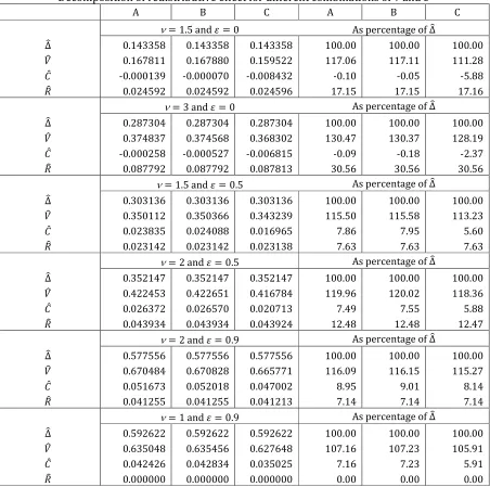
Table 4
Model C thus underestimates the vertical effect by about 3 percent of RE for ν 2 and 0. This underestimation is even larger (somewhat smaller) for ν 1.5 and 0 (ν 3 and 0) and amounts to 5.9 (2.4) percent of RE, as Table 4 indicates. Among the scenarios shown in Table 4,
the differences in the estimates of vertical effect obtained by models C and A (B) are lowest when
ν 2 and 0.9, equaling 0.8 (0.9) percent of RE.
5 CONCLUSION
Models decomposing the redistributive effect of fiscal systems into vertical and horizontal effects
are extensively used by practitioners. The Duclos, Jalbert, and Araar (2003) model, despite its
advantages over some other models, such as the Kakwani’s (1984) and the Aronson, Johnson and
Lambert’s (1994) decompositions of RE, has not yet been broadly employed in empirical research.
The reason may be the relatively complex implementation procedure, which involves
non-parametric methods in estimation of expected post-fiscal incomes.
To override these estimation and calculation difficulties, the designers of the software DAD
19
However, as the application data on the Croatian tax-benefit system indicates, DAD-DJA produces
somewhat inaccurate estimates of EPIs, resulting in biased values of DJA model indices. This paper
carefully explains the estimation procedures needed to obtain the indices of the DJA model, and the
problems occurring in DAD-DJA implementation.
The estimates of expected post-fiscal incomes are obtained by two fitting methods,
kernel-weighted local polynomial regression and Fourier series in trigonometric form. Both achieve
reasonable fit of the data at stake, unlike the method built into DAD-DJA, which seems to
overestimate EPIs at the bottom region of pre-fiscal income distribution. Furthermore, we have
realized that the fitting procedure in DAD-DJA contains a ‘bug’, producing unreasonably high
estimates of EPIs for the top pre-fiscal income units in the sample.
We have shown how the estimation of EPUs can be circumvented, saving a practitioner time
when doing multiple-scenario analysis. Instead of estimating EPUs for each different value of
parameter ε, the index of inequality based on EPUs can be obtained simply by using post-fiscal
incomes ordered according to pre-fiscal incomes. In this procedure, however, caution must be taken
in the presence of large groups of exact pre-fiscal equals: they should all be ascribed identical
20
REFERENCES
Araar, Abdelkrim, and Jean-Yves Duclos. 2003. An Atkinson-Gini Family of Social Evaluation
Functions. Economics Bulletin 3 (19): 1–16.
Araar, Abdelkrim, and Jean-Yves Duclos. 2006. An Atkinson-Gini Family of Social Evaluation
Functions: Theory and Illustration Using Data from the Luxembourg Income Study. Public
Finance 54 (3): 191–209.
Aronson, J. Richard, Paul Johnson, and Peter J. Lambert. 1994. Redistributive effect and unequal
income tax treatment. The Economic Journal 104: 262–270.
Atkinson, Anthony B. 1970. On the Measurement of Inequality. Journal of Economic Theory 2: 244–
263.
Atkinson, Anthony B. 1980. Horizontal Equity and the Distribution of the Tax Burden. In The
Economics of Taxation, Henry J. Aaron, and Michael J. Boskins, eds., 3–18. Washington D.C.:
Brookings Institution.
Bilger, Marcel. 2008. Progressivity, horizontal inequality and reranking caused by health system
financing: A decomposition analysis for Switzerland. Journal of Health Economics 27: 1582–
1593.
Dardanoni, Valentino, and Peter J. Lambert. 2001. Horizontal Inequity Comparisons. Social Choice
and Welfare 18: 799–816.
Donaldson, David, and John A. Weymark. 1980. A Single-Parameter Generalization of Gini indices of
Inequality. Journal of Economic Theory 22: 67–86.
Duclos, Jean-Yves, Abdelkrim Araar, and Carl Fortin. 2010. DAD: A software for Distributive Analysis
/ Analyse Distributive. MIMAP programme, International Development Research Centre,
Government of Canada, and CIRPÉE, Université Laval (version: DAD 4.6 of October 2010).
Duclos, Jean-Yves, Vincent Jalbert, and Abdelkrim Araar. 2003. Classical horizontal inequity and
21
Duclos, Jean-Yves, and Peter J. Lambert. 2000. A Normative and Statistical Approach to Measuring
Classical Horizontal Inequity. Canadian Journal of Economics 33: 87–113.
Ebert, Udo, 1997. Social Welfare When Needs Differ: An Axiomatic Approach. Economica 64: 233–
44.
Ebert, Udo. 1999. Using equivalent income of equivalent adults to rank income distributions. Social
Choice and Welfare 16: 233–258.
Fan, Jianqing, and Gijbels, Irène. 1996. Local polynomial modelling and its applications. London:
Chapman and Hall.
Faunt, Lindsay M., and Michael L. Johnson. 1992. Analysis of discrete, time-sampled data using
Fourier series method. Methods in Enzymology 210: 340–56.
Härdle, Wolfgang. 1990. Applied Nonparametric Regression. Cambridge University Press.
Kakwani, Nanak C. 1984. On the measurement of tax progressivity and redistributive effect of taxes
with applications to horizontal and vertical equity. Advances in Econometrics 3: 149–168.
Keele, Luke. 2008. Semiparametric Regression for the Social Sciences. London: Wiley & Sons.
Plotnick, Robert. 1981. A Measure of Horizontal Equity. The Review of Economics and Statistics 63:
283–288.
Wand, Matt P. and Chris M. Jones. 1995. Kernel Smoothing. London: Chapman and Hall.
Yitzhaki, Shlomo. 1983. On an Extension of the Gini Inequality Index. International Economic Review
24: 617–628.
Yitzhaki, Shlomo, and Ingram Olkin. 1991. Concentration curves and concentration indices. Lecture
22
APPENDIX 1 SAMPLE ESTIMATES OF INEQUALITY INDICES
The sample estimates of Atkinson-Gini Inequality indices based on NY, NX, N& and N' are obtained
in the following equations:
NY, NY / 1 o d NY, ,ν;ωg
N
Y,νf ∑ d
^Y, f ·φ^Y·ωg^Y,ν V
^a
pd NY, ,ν;ωgNY,νf 1 q 1 o d NY, ,ν;ωgNY,νfr
s
stu/!̂ NY (16)
NX, NX / 1
Š d NX, ,ν; bNX,νf ∑V^a d ^X, f ·φ^X· b^X,ν cd NX, ,ν; b
NX,νf 1 q 1 Š d NX, ,ν; bNX,νfr
s
stu/!̂ NX (17)
o d NX, ,ν;ωgNX,νf ∑V^a d ^X, f ·φ^X·ωg^X,ν pd NX, ,ν;ωg
N
X,νf 1 q 1 o d
NX, ,ν;ωgNX,νfr
s
stu/!̂ NX (18)
d N&, f d N&f / 1 o d N&, ,ν;ωg
N
X,νf ∑ d
^&, f ·φ^X·ωg^X,ν V
^a
pd N&, ,ν;ωgNX,νf 1 q 1 o d N&, ,ν;ωgNX,νfr
s
stu/!̂d N&f (19)
o d N,', ,ν;ωgNX,νf ∑V^a N,' ·φ^X·ωg^X,ν
pd N,', ,ν;ωgNX,νf 1 q 1 o d N,', ,ν;ωgNX,νfr
s stu/!̂
NX (20)
where !̂ NY , !̂ NX , and !̂d N&f are means of post-fiscal income variables, equal to !̂ NY
Σ ∑V^a φ^Y· ^Y, !̂ NX Σ ∑^aV φ^X· ^X, and !̂d N&f Σ ∑V^a φ^X· ^&, respectively. It is
clear that !̂ NX !̂ NY , because NX and NY contain the same sample values, only differently
23
ENDNOTES
1 Araar and Duclos (2003, 2006) describe the properties of AGF based inequality indices: “Income
inequality aversion is captured by decreasing marginal utilities, and aversion to rank inequality is
captured by rank-dependent ethical weights, thus providing an ethically-flexible dual basis for the
assessment of inequality and equity” (Araar and Duclos 2006, 192). Furthermore, it is shown that
AGF is the only family of social evaluation functions “to obey a set of popular axioms in the income
distribution literature” (Araar and Duclos 2006, 204).
2 Independent proof of this relationship can be found in Yitzhaki and Olkin (1991), who derive the
“relative concentration curve” of post-fiscal income N with respect to pre-fiscal income X as
$ , “, !* y ” €
" ” ~•ts–
— , where y “ ˜™ | “š corresponds to & . Duclos
and Araar (2006) present the same concentration curve as $ , “, !* – & › ›, from
which the S-Gini concentration coefficient is obtained as I ,ν qd $ , “, frϖ ,ν ,
where ϖ ,ν ν ν 1 1 ν j are rank-dependent weights.
3 These authors have derived their indices using the “cost of inequality” approach, compared with
the “change of inequality” approach used in this paper. Duclos, Jalbert, and Araar (2003) employ
both approaches.
4 According to Ebert (1997, 1999) this is the right approach to investigate the concepts of Lorenz
dominance, social welfare function, and progressive transfers when populations are heterogeneous.
Using the number of ‘real’ household members, œN, instead of the number of ‘equivalent’ members,
PN, leads to “some unpleasant and unsatisfactory paradoxa or impossibility results”. The usual
objection to this approach is that “not all persons have the same weight and significance”, which
contradicts the democratic principles; for the rebuttal of this objection see Ebert (1999, 251).
24
6 Basic support allowances, unemployment benefit, child allowance, sick-leave benefit, maternity
and layette supplement, and supplement for the injured and support for rehabilitation and
25
TABLES
Table 1
Hypothetical population: weight, incomes, and utilities
# bNX ωgNX NX NX NY N& NX NX NY N& N,'
1 (A) 0.438 0.375 10 8 8 12 6.32 5.66 5.66 6.93 6.83
2 (B) 0.313 0.375 10 16 12 12 6.32 8.00 6.93 6.93 6.83
3 (C) 0.188 0.125 20 12 16 18 8.94 6.93 8.00 8.49 8.36
4 (D) 0.063 0.125 20 24 24 18 8.94 9.80 9.80 8.49 8.36
1 1 60 60 60 60 30.54 30.38 30.38 30.83 30.38
[image:26.595.126.471.392.603.2]Note: weights are obtained for ν 2; utilities are obtained for 0.5.
Table 2
Indices obtained for hypothetical population
ν 2
0.5 ν 20
DAD-DJA
ν 2
0
p NX 0.188 0.167 0.167
p NY 0.240 0.217 0.217
c NX 0.210 0.183 0.183
p NX 0.133 0.100
pd N,'f 0.133 0.100
p N& 0.108 0.100 0.500
∆ƒ p NX p NY -0.052 -0.050 -0.050
#ƒ p NX p N& 0.081 0.067 -0.333
$p p NX p
N& 0.026 0.000
%ƒ p NY p
NX 0.107 0.117
$c c NX p
N& 0.102 0.083 -0.317
26 Table 3
Decomposition of redistributive effect for ν 2 and 0
A B C A B C
As percentage of p NX
p NX 0.506665 0.506665 0.506665 100.00 100.00 100.00
p NY 0.291511 0.291511 0.291511 57.54 57.54 57.54
c NX 0.244328 48.22
p NX 0.244337 0.244337 48.22 48.22
p N& 0.244540 0.244517 0.251432 48.26 48.26 49.62
As percentage of ∆ƒ
∆ƒ 0.215154 0.215154 0.215154 100.00 100.00 100.00
#ƒ 0.262124 0.262148 0.255233 121.83 121.84 118.63
$p -0.000203 -0.000180 -0.007104 -0.09 -0.08 -3.30
%ƒ 0.047174 0.047174 0.047183 21.93 21.93 21.93
27 Table 4
Decomposition of redistributive effect for different combinations of ν and
A B C A B C
ν 1.5 and 0 As percentage of ∆ƒ
∆ƒ 0.143358 0.143358 0.143358 100.00 100.00 100.00
#ƒ 0.167811 0.167880 0.159522 117.06 117.11 111.28
$p -0.000139 -0.000070 -0.008432 -0.10 -0.05 -5.88
%ƒ 0.024592 0.024592 0.024596 17.15 17.15 17.16
ν 3 and 0 As percentage of ∆ƒ
∆ƒ 0.287304 0.287304 0.287304 100.00 100.00 100.00
#ƒ 0.374837 0.374568 0.368302 130.47 130.37 128.19
$p -0.000258 -0.000527 -0.006815 -0.09 -0.18 -2.37
%ƒ 0.087792 0.087792 0.087813 30.56 30.56 30.56
ν 1.5 and 0.5 As percentage of ∆ƒ
∆ƒ 0.303136 0.303136 0.303136 100.00 100.00 100.00
#ƒ 0.350112 0.350366 0.343239 115.50 115.58 113.23
$p 0.023835 0.024088 0.016965 7.86 7.95 5.60
%ƒ 0.023142 0.023142 0.023138 7.63 7.63 7.63
ν 2 and 0.5 As percentage of ∆ƒ
∆ƒ 0.352147 0.352147 0.352147 100.00 100.00 100.00
#ƒ 0.422453 0.422651 0.416784 119.96 120.02 118.36
$p 0.026372 0.026570 0.020713 7.49 7.55 5.88
%ƒ 0.043934 0.043934 0.043924 12.48 12.48 12.47
ν 2 and 0.9 As percentage of ∆ƒ
∆ƒ 0.577556 0.577556 0.577556 100.00 100.00 100.00
#ƒ 0.670484 0.670828 0.665771 116.09 116.15 115.27
$p 0.051673 0.052018 0.047002 8.95 9.01 8.14
%ƒ 0.041255 0.041255 0.041213 7.14 7.14 7.14
ν 1 and 0.9 As percentage of ∆ƒ
∆ƒ 0.592622 0.592622 0.592622 100.00 100.00 100.00
#ƒ 0.635048 0.635456 0.627648 107.16 107.23 105.91
$p 0.042426 0.042834 0.035025 7.16 7.23 5.91
28
[image:29.595.70.528.162.419.2]FIGURES
Figure 1
Scattergram of pre- and post-fiscal incomes
0 0.2 0.4 0.6 0.8 1 0.0 0.5 1.0 1.5 2.0 2.5
0.0 0.5 1.0 1.5 2.0 2.5
C u m u la ti v e d en si ty P o st -f is ca l in co m e Pre-fiscal income
Series1 EPIs CD
Notes: (a) each point represents one sample income unit; (b) EPIs – expected post-fiscal incomes
29 Figure 2
Scattergram of pre- and post-fiscal incomes
0.0 0.5 1.0 1.5 2.0 2.5
0.0 0.5 1.0 1.5 2.0 2.5
P
o
st
-f
is
ca
l
in
co
m
e
Pre-fiscal income Series1 A B C
Note: (a) each point represents one sample income unit; (b) A, B, and C – estimates of expected
post-fiscal incomes obtained by KWLPR, FTTF, and DJA-LLE fitting methods, respectively (see details in