A space time generator for rainfall nowcasting: the PRAISEST model

www.hydrol-earth-syst-sci.net/13/441/2009/ © Author(s) 2009. This work is distributed under the Creative Commons Attribution 3.0 License.

Earth System

Sciences

A space-time generator for rainfall nowcasting: the PRAISEST

model

P. Versace, B. Sirangelo, and D. L. De Luca

Dipartimento di Difesa del Suolo, Universit`a della Calabria, Rende, Italy

Received: 22 January 2008 – Published in Hydrol. Earth Syst. Sci. Discuss.: 18 March 2008 Revised: 3 February 2009 – Accepted: 25 March 2009 – Published: 7 April 2009

Abstract. The paper introduces a stochastic technique for

forecasting rainfall in space-time domain: the PRAISEST Model (Prediction of Rainfall Amount Inside Storm Events: Space and Time). The model is based on the assumption that the rainfall heightH accumulated on an interval1t be-tween the instantsi1tand(i+1) 1tand on a spatial cell of size1x1y is correlated either with a variableZ, represent-ing antecedent precipitation at the same point, either with a variableW, representing simultaneous rainfall at neighbour cells. The mathematical background is given by a joined probability densityfH,W,Z(h, w, z)in which the variables

have a mixed nature, that is a finite probability for null value and infinitesimal probabilities for the positive values. As study area, the Calabria region, in Southern Italy, has been selected. The region has been discretised by 10 km×10 km cell grid, according to the raingauge network density in this area. Storm events belonging to 1990–2004 period were an-alyzed to test performances of the PRAISEST model.

1 Introduction

The risk mitigation in landslide or flood prone areas is one of the most important topics in environmental sciences. In the next future this relevance will increase owing to the devel-opment of mitigation and adaptation policies related to cli-matic change (Stern, 2006; IPCC, 2007). In this scenario the non structural measures, mainly based on early warning system, will play, increasingly, a relevant role. So all the related hydrological topics like rainfall-runoff modelling or rainfall-landslide relationships will be also developed, with the general scientific aim of realizing an accurate simulation of the real phenomena, but also in order to forecast landslide

Correspondence to: D. L. De Luca ([email protected])

and flood events with a lag time large enough for activating civil protection measures.

Indeed, in all the cases where the phenomenon rapidly evolves, like flash floods or shallow landslides, the lag time between observed rainfall and flood or landslide occurrence results too short and must be extended by rainfall fields fore-casting. This is the main reason for the rise of the interest in this topic (Reed et al., 2007; Bloschl et al., 2008).

In the technical literature rainfall forecasting models can be classified in time stochastic models, space-time stochastic models and meteorological ones.

In the first class, we consider the “discrete time-series models”, that include AutoRegressive Stochastic Models (Box and Jenkins, 1976; Toth et al., 2000). They describe the rainfall process at discrete time steps, are not intermit-tent and therefore can be applied for describing the “within storm” rainfall. Space-temporal stochastic models can be classified in Multivariate models and Multidimensional ones. The former consider several rain gauges simultaneously and are intended to preserve the covariance structure of the his-torical rainfall data existing in the network points. On the temporal axis, forecasting is made by autoregressive scheme (STARMA and CARMA models, Cliff et al., 1975; Burlando et al., 1996).

The latter models attempt to characterize the rainfall phe-nomenon at every point over the area of interest (Bras and Rodriguez-Iturbe, 1984; Meiring et al., 1997).

Finally, meteorological models (Untch et al., 2006) solve in numerical way partial differential equations of atmosphere thermodynamics: they can be classified in GCM (Global Cir-culation Models) and LAM (Limited Area Models).

the precision of this kind of models also decrease (Koussis et al., 2003; Bartholmes and Todini, 2005; Sharma et al., 2007). Unfortunately this is the time space scale of the fast phenomena (flash floods and shallow landslide) that require rainfall forecast for civil protection measures. Then it is not plenty profitable to rely on meteorological models for quan-titative rainfall forecasting, as the probability of both missed and false alarms may be too large.

Consequently, in order to perform short term real-time rainfall forecasts for small basins (i.e. with size ranging 100– 1000 km2), stochastic models appear to be competitive, as they take account of the hydrological characteristics of the investigated area.

Nevertheless, stochastic models input is only constituted by antecedent rainfalls, so they provide the same prevision, whether meteorological models forecast a wet period or a dry one. For these reasons, coupling stochastic and meteo-rological models appears a very interesting topic for rainfall forecasting in the small time space scale (Di Tria et al., 1999; Sirangelo et al., 2006).

This work introduces a space-temporal models to fore-cast rainfall fields named PRAISEST (Prediction of Rainfall Amount Inside Storm Events: Space and Time). It is a mul-tidimensional space-time model, that can be considered like the generalization of the at-site model PRAISE proposed by the authors (Sirangelo et al., 2007).

PRAISEST is based on the assumption that the evaluation rainfall heightH, accumulated over an interval1t and on a spatial cell of size1x1y, depends on antecedent precipita-tion at the same site, and on rainfalls of neighbour cells.

In the following Sections the theoretical bases of the pro-posed model (Sect. 2), fitting techniques (Sect. 3) and rainfall generation algorithm (Sect. 4) are discussed. The application of the model to the case study of Calabria region, in Southern Italy, is reported in Sect. 5.

2 The PRAISEST Model

2.1 Identification of random variables

In the PRAISEST model there are three fundamental random variables:

a)Hi+1, defined as the rainfall height on the forecasting interval1tbetween the instantsi1tand(i+1) 1t for a cell having area1x1y.

b) for a fixed lag in time,ν, and for a given pixel where the future rainfallHi+1must be estimated, construct the au-toregression of rainfall heights

Z_i(ν)=

ν−1

X

j=0

αjHi−j (1)

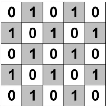
Fig. 1. PRAISEST Scheme for each pixel.

whereαj are autoregressive coefficients to be estimated for

each lag, with the conditions 0<αj≤1, forj=0,1, ..., ν−1,

and

ν−1

P

j=0 αj=1.

c)Wi+1, defined as a weighted average of rainfall heights over the four closest neighbouring pixels:

Wi+1= 4

X

j=1

β_j0H_i(j )₊₁ (2)

where the superscript indicates the pixel in the neighbour-hood, as shown in Fig. 1.

Considering larger neighbourhoods or a different weight-ing procedure, to allow for either anisotropy or influence from a larger region, implies a greater number of parameters and gives us similar results.

As regardsZ(ν)_i , the linear stochastic dependence between the random variable Hi+1 and the generic antecedent ran-dom variablesHi−j,j=0,1,2, ..., i.e. the extension of the

temporal “memory”ν of the rain field, for every cell, can be assumed equal to the minimum value ofν for which the sample maximum absolute scatteringχr(ν)(Sirangelo et al.,

2007) results less than a fixed critical valueχr,cr.

The coefficientsαj can be estimated by maximization of

the coefficient of linear correlation ρ Hi+1Zi(ν)

of linear filtering results convenient, as the coefficients αj

depend on a reduce number of parameters.

In this paper, the gamma-power function is used as filter (De Luca, 2005), depending on three parameters, that pro-vides a good fitting of the estimated values ofαj.

Then, the coefficientsαjcan be calculated as:

αj =

Pa, ((j+1)b1t )c−Pa, (j b1t )c

Pa, (ν b1t )c (3)

whereP (a, x)= 1

0(a) x R

0

e−tta−1dtis the incomplete gamma function (Abramowitz and Stegun, 1970).

More precisely, for every set (a, b, c), the sample vari-ablez(ν)_i ,i = ν, ν+1, ..., N −1, can be evaluated and then the optimal valuesa,ˆ b,ˆ cˆcan be obtained by maximizing the sample linear correlation coefficientrH Z betweenHi+1and Z_i(ν). A numerical procedure (Press et al., 1988) is adopted.

As regards the random variableWi+1, theβ

0

j coefficients

can be evaluated as:

β_j0 = ρ

0

j,0 4

P

j=1 ρ_j,0 ₀

j=1,2,3,4 (4)

andρ₁0_,0, ρ₂0_,0, ρ₃0_,0, ρ₄0_,0indicate the linear correlation coef-ficients between the reference cell 0 and the neighbour cells 1, 2, 3 and 4 (Fig. 1).

Obviously if the field can be considered locally isotropic, the coefficientsβ_j0 assume the same value equal to 1/4.

For each pixel the aim is then to predict the rainfall to-tal Hi+1 at a subsequent timestep considering the triple

Hi+1, Wi+1, Z(ν)i

, where Wi+1 is a weighted average at the forecast timestep and this results in a implicit scheme. Section 4 outlines a methodology for using this scheme in the forecasting of rainfall fields.

The PRAISEST Model can be used considering several temporal and spatial scales, according to the available rainfall data. In the case of high-resolution timestep, for example hourly or sub-hourly, storm advection may be reproduced, in stochastic way, by the correlation structure referred to the spatial neighbourhood approach.

In the following, for notation simplicity, the subscripts of random variablesH,WandZwill be removed where possi-ble.

2.2 Structure of the joint and conditional probability density

Starting from the joint probability densityfH,W,Z(h, w, z)is

important for deriving the expression of the conditional one fH|W,Z(h|w, z), used to forecast rainfall fields.

To identifyfH,W,Z(h, w, z)it is necessary to consider the

mixed nature of random variablesH,W andZ. All the three

variables are non-negative and characterized by a finite prob-ability in correspondence of the null value and by infinitesi-mal probabilities in correspondence of the positive values.

Then, indicated with pH,W,Z, pH,W,0, pH,0,Z, p0,W,Z, pH,0,0,p0,W,0,p0,0,Zandp0,0,0the probabilities associated, for each pixel, to the events:

H >0∩W >0∩Z>0, H >0∩W >0∩Z=0, H >0∩W=0∩Z>0, H=0∩W >0∩Z>0, H >0∩W=0∩Z=0, H=0∩W >0∩Z=0, H=0∩W=0∩Z>0,

H=0 ∩ W=0 ∩ Z=0, the joint probability density fH,W,Z(h, w, z)assumes the form:

fH,W,Z(h, w, z)=p0,0,0δ (h) δ (w) δ (z)+

pH,0,0·gH,0,0(h)·δ (w) δ (z)+ p0,W,0·g0,W,0(w)·δ (h) δ (z)+ p0,0,Z·g0,0,Z(z) δ (h) δ (w)+ pH,W,0·gH,W,0(h, w) δ (z)+ pH,0,Z·gH,0,Z(h, z) δ (w)+ p0,W,Z·g0,W,Z(w, z) δ (h)+ pH,W,Z·gH,W,Z(h, w, z)

(5)

where the symbolδ (·)indicates the Dirac’s delta function and:

gH,W,Z(h, w, z) dhdwdz= (6)

Pr [h≤H <h+dh∩w≤W < w+dw∩z≤Z<z+dz| H >0∩W >0∩Z>0]

gH,W,0(h, w) dhdw= (7)

Pr [h≤H < h+dh∩w≤W < w+dw| H >0∩W >0∩Z=_0]

gH,0,Z(h, z) dhdz= (8)

Pr [h≤H < h+dh∩z≤Z < z+dz| H >0∩W =0∩Z >0]

g0,W,Z(w, z) dwdz= (9)

Pr [w≤W < w+dw∩z≤Z < z+dz| H=0∩W >0∩Z >0]

gH,0,0(h) dh= (10)

g0,W,0(w) dw= (11) Pr [w≤W < w+dw|H =0∩W >0∩Z=_0]

g0,0,Z(z) dz= (12)

Pr [z≤Z < z+dz|H =0∩W =0∩Z >0]

and clearly, p0,0,0+pH,0,0+p0,W,0+p0,0,Z+pH,W,0 + pH,0,Z+p0,W,Z+pH,W,Z=1.

The conditional distribution fH|W, Z(h|w, z), necessary

to perfom the forecasting, is characterized by four separate cases, due toW null or positive andZnull or positive.

Considering the cumulative distribution function (CDF) FH|W,Z(h|w, z), we obtain the following expressions:

– ifW=0 andZ=0 then FH|W,Z(h|w, z)=

p0,0,0+pH,0,0GH,0,0(h) p0,0,0+pH,0,0

(13a) whereGH,0,0(h)is the CDF ofgH,0,0(h)and the probability referred to the eventH=0|W=0∩Z=0 is:

p0,0,0 p0,0,0+pH,0,0

(13b)

– ifW >0 andZ=0 then

FH|W,Z(h|w, z)= (14a)

p0,W,0·g0,W,0(w)+pH,W,0·GH|W,0(h|w)·gW(w) p0,W,0·g0,W,0(w)+pH,W,0·gW(w)

whereGH|W,0(h|w)is the CDF of the conditional density gH|W,0(h|w), gW(w)is the marginal density with the

re-spect toW, derived fromgH,W,0(h, w), and the probability referred to the eventH=0|W >0∩Z=0 is:

p0,W,0·g0,W,0(w)

p0,W,0·g0,W,0(w)+pH,W,0·gW(w)

(14b)

– ifW=0 andZ>0 then

FH|W,Z(h|w, z)= (15a)

p0,0,Z·g0,0,Z(z)+pH,0,Z·GH|0,Z(h|z)·gZ(z) p0,0,Z·g0,0,Z(z)+pH,0,Z·gZ(z)

whereGH|0,Z(h|z) is the CDF of the conditional density gH|0,Z(h|z),gZ(z)is the marginal density with the respect

toZ, derived fromgH,0,Z(h, z), and the probability referred

to the eventH=0|W=0∩Z>0 is: p0,0,Z·g0,0,Z(z)

p0,0,Z·g0,0,Z(z)+pH,0,Z·gZ(z)

(15b)

– ifW >0 andZ>0 then

FH|W,Z(h|w, z)= (16a)

p0,W,Z·g0,W,Z(w, z)+pH,W,Z·GH|W,Z(h|w, z)·gW,Z(w, z)

p0,W,Z·g0,W,Z(w, z)+pH,W,Z·gW,Z(w, z)

whereGH|W,Z(h|w, z)is the CDF of the conditional density gH|W,Z(h|w, z), gW,Z(w, z) is the marginal density with

the respect toWandZ, derived fromgH,W,Z(h, w, z), and

the probability referred to the eventH=0|W >0∩Z>0 is: p0,W,Z·g0,W,Z(w, z)

p0,W,Z·g0,W,Z(w, z)+pH,W,Z·gW,Z(w, z)

(16b) In each case reported in Eqs. (6–12) the marginal distribu-tion of the positive variablesH,W andZ will be assumed to follow a Weibull distribution FX(x)=1−exp(−λxη),

where the parameters λ and η can be estimated via the method of moments.

It is important to emphasise that each conditioning case will have different power transformation parameters, as the distribution of one variable differs depending on whether the other variables are positive or zero. Moreover, the whole en-semble of parameters varies from a pixel to each other. After performing a power transformation, to model the joint den-sity of the variables it suffices to consider multivariate expo-nential distributions (Kotz et al., 2000). The Moran-Dowton multivariate exponential distribution for a vectorXhavingp unit mean marginals is written as:

fX x

= (17)

θp−1exp −θ·

p X

i=1 xi

!

·Sp "

(θ−1) θ(p−1)·

p Y

i=1 xi

#

whereθis an association parameter that is the same between all dimensions and where

Sp[q]= ∞ X

r=0 qr

(r!)p (18)

The Eq. (17) is characterized by exponential marginal den-sity functions. The association parameter respect the condi-tionθ ≥ 1 and it is related to the linear correlation coeffi-cient between any two variablesXi andXj asρi,j=1−1θ.

Consequently, ifθ=1 thenρi,j =0 and the Eq. (17) can be

written as:

fX x

=exp −

p X

i=1 xi

!

=

p Y

i=1

exp(−xi) (19)

that implies the independence among the random variables. From the Eq. (17) the conditional densitygH|W,Z(h|w, z)

gH|W,Z(h|w, z)= (20) gH,W,Z(h, w, z)

gW,Z(w, z)

=θhwzλhηhhηh−1exp −θhwzλhhηh

· S3(θhwz−1) θ_hwz2 λhhηhλwwηwλzzηz

S2(θhwz−1) θhwzλwwηwλzzηz

where(λh, ηh), (λw, ηw), (λz, ηz)are the power

transfor-mation parameters, respectively, forh,w, z andθhwzdenotes

that the association parameter is estimated from the observa-tions(h>0, w>0, z>0). Asθhwzis the same in each

dimen-sion it is evaluated from all of the pairs within this group (h, w), (h,z), and (w,z).

The conditional densitygH|W,0(h|w)can be written as:

gH|W,0(h|w)=

gH,W,0(h, w) gW(w)

= (21)

θhwλhηhhηh−1exp −θhwzλhhηh

· S2(θhw−1) θhwλhhηhλwwηw

where the power transformation parameters (λh, ηh), (λw, ηw)are different from those of Eq. (20) because they

are evaluated from the observations(h>0, w>0, z=0); the same ensemble of observations is used for theθhw

estima-tion.

A similar expression forgH|0,Z(h|z)can be developed

re-quiring a separateθhzthat is estimated from the recordered

data(h>0, w=0, z>0). Starting from Eq. (17), it is easily to determine the structure of the probability density function g0,W,Z(w, z), whilegH,0,0(h),g0,W,0(w)andg0,0,Z(z)are

simply the univariate Weibull distributions and do not require any additional parameters apart from the power transforma-tion ones.

3 Model calibration

The trivariate probability distribution function fH,W,Z(h, w, z) presents 42 parameters for every pixel.

This number is not too large, if we consider that in 10 years there are 87 600 hourly data (supposing that the rainfall process is stationary in time during the whole year) related to every cell, i.e. the d/p (data/parameters in a generic cell) ratio is approximatively equal to 2050, and remains high enough (about 150) also if positive rainfall data are only considered. Using raingauge data and cells domain the ratio does not change if the number of stations and cells are similar.

This d/p ratio value allows consistent evaluations of PRAISEST parameters referred to the whole spatial domain. The first calibration step, for every cell, is the evaluation of (a, b, c) by numerical technique. Estimation ofβ_j0,j=1, 2, 3,

4, follows by analyzing sample linear correlation coefficient r₁0_,0, r₂0_,0, r₃0_,0, r₄0_,0.

The probabilitiespH,W,Z,pH,W,0,pH,0,Z,p0,W,Z,pH,0,0, p0,W,0andp0,0,Zcan be estimated by the frequencies of the

corresponding events.

The power transformation parameters referred to the prob-ability densities of the Eq. (5) can be estimated by using classic expressions of Weibull distribution parameters esti-mation, referred to the method of moments.

The estimation of the association parameterθhwz, is

per-formed minimizing the following function:

R (θhwz)= (22)

ω1(ρH W −rH W)2+ω2(ρH Z−rH Z)2+ω3(ρW Z−rW Z)2

whererH W,rH Z,rW Zare the sample linear correlation

coef-ficients, and the sum of the weightsω1,ω2andω3is unitary. The Eq. (22) depends only on the parameterθhwz, since the

remaining parameters have been evaluated in a previous step. With similar procedures, the association parameters of the remaining density functions of Eq. (5) can be evaluated.

4 Rain fields generation algorithms

The generation of the rainfall heights on the entire domain differs from the standard Monte Carlo approach. In fact, at the current timei, the values of the random variableZi in

every cell are known, but values ofWi+1 andHi+1 on the entire domain must be generated. Such generations cannot be carried out independently cell by cell, because the variables are linked by congruence equations. This problem has been solved using the following “Chess-Board” algorithm (Fig. 2): 1. for every “0” cells of the spatial domain, know-ing the value of Zi, generation is made

us-ing the random number R(_U0), by the formula h_i(0₊)₁=F_H−_|1_ZR_U(0)|W_i(₊0)₁≥0, Z_i(0)=z(_i0), i.e. the vari-ableHi+1is generated supposing zero as lower bound for Wi+1. The formulation of the densityFH|Z(h|z),

marginal with respect to W and conditional with re-spect toZ, is easily obtained from the Eq. (5). This type of generation is justified because, in the model, rainfall heights in the “0” cells are each other independent. 2. As regards the “1” cells, knowing the value of

Zi, W_i(+1)1 is set equal to the linear combination of the H_i(₊0)₁ in the neighbours “0” cells. Con-sequently, generation is made by the formula h(_i1₊)₁=F_H−_|1_W,ZR(_U1)|W_i(₊1)₁=w(_i1₊)₁, Z_i(0)=z(_i0) us-ing the random numberR(_U1).

Fig. 2. “Chess-Board” algorithm.

5 Application

5.1 Parameters estimation

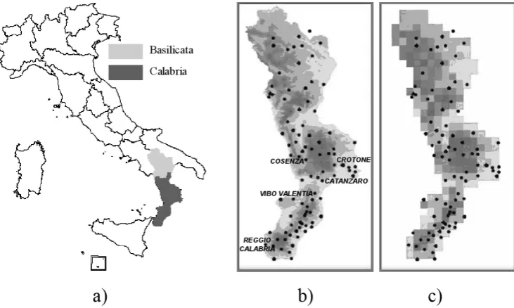
PRAISEST model has been applied using the hourly rain heights database of the tele-metering raingauge network of the “Centro Funzionale Meteorologico Idrografico Mare-ografico” of the Calabria region. The network, extended all over the Calabria and Basilicata regions has 92 stations for the period 1990–2001, and 126 stations from 2002 to 2004 (Fig. 3). Approximately, 13 million of hourly rainfalls form the database, of which about 7% are rainy.

The region was discretized by 10 km×10 km cell grid, ac-cording to the raingauge network density.

In order to respect the hypothesis of stationary process, only the data measured during the “rainy season”, 1 October– 31 May have been used (De Luca, 2005). In this period, correlation structure, mean and variance of the sample appear significantly homogeneous (Sirangelo et al., 2007). So the d/p ratio is equal to about 2050 and about 150 considering only rainy intervals.

The historical series do not refer to a regular mesh, so the model parameters have been estimated for every raingauge and then mapped on the regular discretized domain by using a surface spline technique (Yu, 2001).

The extension of the “temporal memory”, i.e. the param-eter ν, has been determined for every raingauge starting from sample partial autocorrelogram, and using the tech-nique cited at point 2.1 (Sirangelo et al., 2007). The value of χr,crhas been fixed equal to 0.025, and the estimate ofνhas

beenνˆ=8, as depicted in Fig. 4, where the mean value of the scatteringχr(ν), considering all the telemeter-raingauges, is

represented.

The coefficientsαj have been calculated, for every

rain-gauge, applying the gamma-power function as filter (Eqs. 2– 3).

For the evaluation of coefficientsβ_j0 definingWi+1(Eq. 4), sample directional spatial correlograms have been analysed, using simultaneous rainfall, and considering, on abscissa, distance between raingauges over the range [5 km; 15 km], representing spatial resolution of the region, discretized by 10 km×10 km cell grid. Four circular sectors of 90 degrees, centred in the NE, SE, SW, NW directions have been consid-ered. Sample correlation values appear to be independent on the directions, as depicted in Fig. 5, so the rain fields can be considered as local isotropic, and thenβ_j0=1/4,j=1, 2, 3, 4. Table 1 reports a set of estimated parameters, evaluated as described in Sect. 3.

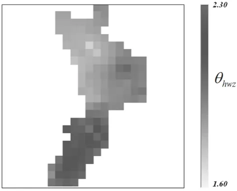
Figure 6 shows an example of parameter mapping in Cal-abria region, referred toθhwz, forH >0∩W >0∩Z>0 event.

Greater values are located in the Southern Calabria, so in this area the variablesH,W andZ appear more strongly corre-lated.

5.2 Model validation

The hourly scattered data, referred to raingauges network, have been interpolated, by a surface spline technique, on reg-ular mesh, of 10×10 km square cells.

Each rain field simulation requires the knowledge of the rainfalls during the eight previous hours, equal to the tem-poral memory. The rain field simulations can be carried out for the successive hours, but the temporal extension of the forecasting should not exceed six hours, to avoid rainfall es-timations based on only simulated precipitations. Beyond this limit the uncertainty in rainfall evaluation increases, as the influence of recorded rainfall decreases.

In the application here described, 10 000 simulations of the process have been carried out, by Monte Carlo technique de-scribed in Sect. 4, in order to obtain a large synthetic sample, necessary to determine probabilistic distribution of rainfall height for every pixel and for each hour. The Monte Carlo technique is adopted because of the complexity of determin-ing analytical probabilistic distributions for forecast rainfall during the hours successive to the first one. For these distri-butions, convolution operations are required.

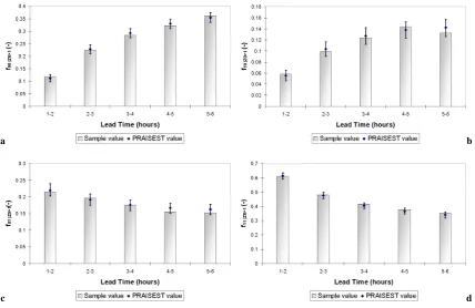
Firstly, the validation is carried out focusing our attention on the ensemble of events inside the storm development char-acterized byZ0>1 mm (where the subscript “0” is related the eight previous hours of recorded data), which are of major interest for our approach, and then testing the model perfor-mance on reproducing, for each of the successive six hours of forecasting, the following sample moments which are not fitted in the parameters estimation:

– meanmH|Z0>1and standard deviationssH|Z0>1;

Fig. 3. (a) Location of Basilicata and Calabria regions; (b) Rainguage network; (c) Discretization of spatial domain.

Table 1. Example of estimated parameters set.

event p(−) 1

λh(mm) ηh(−) 1λw(mm) ηw(−) 1λz(mm) ηz(−) θ(−)

H >0∩W >0∩Z>0 0.062 1.27 0.76 1.25 0.81 1.10 0.75 1.94

H >0∩W >0∩Z=0 0.008 0.81 0.66 0.83 0.73 2.12

H >0∩W=0∩Z>0 0.013 0.61 0.66 0.61 0.65 1.75

H=0∩W >0∩Z>0 0.034 0.46 0.64 0.44 0.56 1.16

H >0∩W=0∩Z=0 0.005 0.46 0.63

H=0∩W >0∩Z=0 0.028 0.45 0.59

H=0∩W=0∩Z>0 0.107 0.26 0.46

Fig. 4. Evaluation of temporal memory extension.

– dry ratios f00|Z0>1, wet-to-dry f10|Z0>1, dry-to wet f01|Z0>1and wet-to-wetf11|Z0>1ratios for two subse-quent images.

The number of events is about 2000 and the results are reported in Figs. 7–8, in which the histograms represent the

sample values averaged on the whole spatial domain. More-over for each index, mean value and 95% band of PRAISEST simulations are reported. The figures demonstrate the over-all capability of the method to reproduce the rainfover-all fields properties.

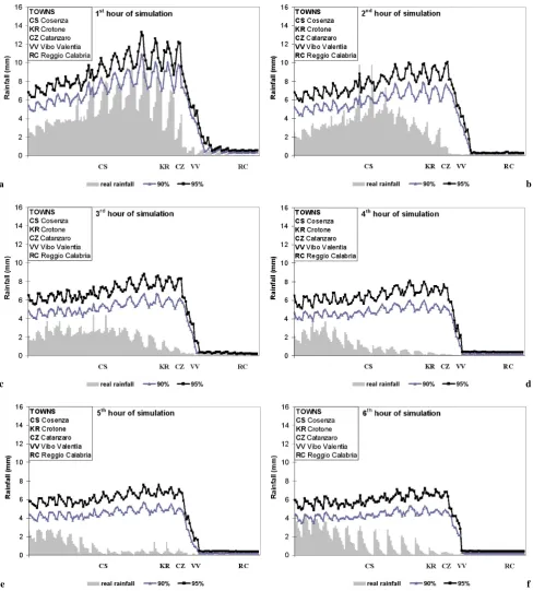
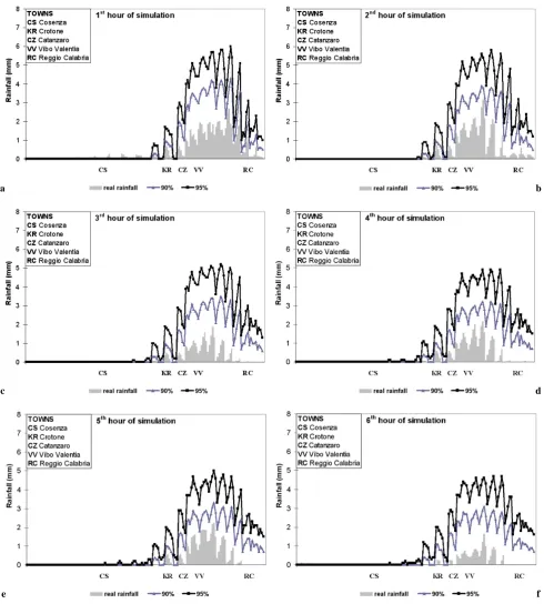
Moreover, as examples of model output, the applications relative to 1 February 1998 and 24 November 1999 events in the Calabria region are illustrated in Figs. 9–10.

Fig. 5. Sample directional spatial correlograms.

Fig. 6. Mapping of the parameterθhwz.

Cosenza (CS), Crotone (KR), Catanzaro (CZ), Vibo Valentia (VV) and Reggio Calabria (RC) are met in this order. One tail significance test, at 5% and 10% significance level, has been performed. The diagrams show that observed rainfall for all, but one, cells are inferior to percentiles 95% of fore-cast values. In the most cases observed values are also in-ferior to percentiles 90% of forecast ones. Then in all cases the results obtained by PRAISEST model seem in agreement with observed data.

6 Conclusions

The PRAISEST model, presented herein, is a multidimen-sional space-time model for forecasting rainfall fields. Math-ematical background is characterized by a trivariate

proba-bility distribution, referred to the random variablesH,Zand W, representing rainfall to forecast at the generic cell, an-tecedent precipitation in the same cell and rainfall in the ad-jacent cells.

The results in simulation at regional scale show the capa-bility of the model to reproduce, for each forecasting hour, mean and standard deviations values, autocorrelations and spatial correlations, dry ratios, wet-to-dry, dry-to-wet and wet-to-wet ratios for two subsequent images.

Consequently it is able to provide distribution functions of the rainfall in the successive hours that are in agreement with the observed values, at least at 10% significance level.

PRAISEST therefore can be easily coupled with other models like rainfall-runoff and rainfall-landslide ones for nowcasting of fast phenomena, characterized by short lag time, like flash floods and shallow landslides.

Moreover the model is highly flexible and can be usefully adopted with any cell grid, within the limit of the raingauge density. Then it is very suitable for the analysis of spatial rainfall data like the radar derived ones, which give a finer spatial description of the precipitation fields. Radar data are, in fact, compatible with the cell organization of the PRAIS-EST spatial domain.

The proposed model also seems appropriate for coupling with meteorogical models in order to realize a Bayesian approach to rainfall nowcasting.

a b

c d

Fig. 7. Validation results for (a) mean valuemH|Z0>1; (b) standard deviation valuesH|Z0>1; (c) spatial correlationrH W|Z0>1; (d) autocor-relation of lag 1r1|Z0>1.

a b

c d

a b

c d

e f

a b

c d

e f

References

Abramowitz, M. and Stegun, I. A.: Handbook of mathematical functions, Dover, New York, NY, USA, 1970.

Bartholmes, J. and Todini, E.: Coupling meteorological and hydro-logical models for flood forecasting. Hydrol. Earth Syst. Sci. 9, 333–346, 2005.

Bloschl, G., Reszler, C., and Komma, J.: A spatially distributed flash flood forecasting model. Environ. Model. Soft. 23, 464– 478, 2008.

Box, G. E. P. and Jenkins, G. M.: Time series analysis: forecasting and control. Holden-Day, S. Francisco, 1976.

Bras, R. L. and Rodriguez-Iturbe, I.: Random functions and hydrol-ogy, Dover Publications, 1984.

Brockwell, P. J. and Davis, R. A.: Time Series. Theory and Meth-ods, Springer Verlag, New York, NY, USA, 1987.

Burlando, P., Montanari, A., and Ranzi, R.: Forecasting of storm rainfall by combined use of radar, rain gages and linear models. Atmos. Res., 42, 199–216, 1996.

Cliff, A. D., Hagget, P., Ord, J. K., Bassett, K. A., and Davies, R. B.: Elements of Spatial Structure: A Quantitative Approach, Cambrige University Press, 1975.

De Luca, D. L.: Metodi di previsione dei campi di pioggia. Tesi di Dottorato di Ricerca, Universit`a della Calabria, Italy, 2005. Di Tria, L., Grimaldi, S., Napolitano, F., and Umbertini, L.:

Rain-fall forecasting using limited area models and stochastic models, Proc. of EGS Plinius Conference, Maratea, 193–204, 1999 IPCC (Inter Governmental Panel on Climate Change): Climate

Change 2007: Mitigation, Cambridge University Press, 2007. Kotz, S., Balakrishanan, N., and Johnson, N.L.: Continuous

Mul-tivariate Distributions – Models And Applications. Wiley, New York, NY, USA, 2000.

Koussis, A. D., Lagouvardos, K., Mazi, K., Kotroni, V., Sitzmann, D., Lang, J., Zaiss, H., Buzzi, A., and Malguzzi, P.: Flood Forecasts for Urban Basin with Integrated Hydro-Meteorological Model, J. Hydrologic Eng., 8(1), 1–11, 2003.

Meiring, W., Monestiez, P., Sampson, P. D., and Guttorp, P.: De-velopments in the modelling of nonstationary spatial covari-ance structure from space-timing monitoring data. In Baafi and Schofield editors, Geostatistics Wollongong ‘96, Kluver, Dor-drecht, The Netherlands, 162–173, 1997.

Press, W. H., Flannery, B. P., Teukolsky, S. A., and Vetterling, W. T.: Numerical Recipes in C. The art of scientific computing, Cam-brige University Press, 1988.

Reed, S., Schaake, J., and Zhang, Z.: A distributed hydrologic model and threshold frequency-based method for flash flood forecasting at ungauged locations, J. Hydrol., 337, 402–420, 2007.

Sharma, D., Das Gupta, A., and Babel, M. S.: Spatial disaggre-gation of bias-corrected GCM precipitation for improved hydro-logic simulation: Ping River Basin, Thailand, Hydrol. Earth Syst. Sci., 11, 1373–1390, 2007,

http://www.hydrol-earth-syst-sci.net/11/1373/2007/.

Sirangelo, B., Versace, P., De Luca, D. L.: Rainfall nowcasting: in-tegrazione bayesiana di modelli stocastici e meteorologici. Atti del XXX Convegno di Idraulica e di Costruzioni Idrauliche, Roma, 2006.

Sirangelo, B., Versace, P., De Luca, D. L.: Rainfall nowcasting by at site stochastic model P.R.A.I.S.E. Hydrol. Earth Syst. Sci. 11, 1341–1351, 2007.

Stern, N.: The Economics of Climate Change The Stern Review, Cambridge University Press, 2006.

Toth, E., Brath, A., and Montanari, A.: Comparison of short-term rainfall prediction models for real-time flood forecasting. J. Hy-drol., 239(1), 132–147, 2000.

Untch, A., Miller, M., Hortal, M., Buizza, R., and Janssen, P.: To-wards a global meso-scale model: the high-resolution system TL799L91 and TL399L62 EPS. Newsletter n. 108, ECMWF, Shinfield Park, Reading RG2-9AX, UK, 2006.