Reviving the “Ganges Water Machine”: where and how much?

www.hydrol-earth-syst-sci.net/21/2545/2017/ doi:10.5194/hess-21-2545-2017

© Author(s) 2017. CC Attribution 3.0 License.

Reviving the “Ganges Water Machine”: where and how much?

Lal Muthuwatta1, Upali A. Amarasinghe1, Aditya Sood1, and Lagudu Surinaidu2

1_{International Water Management Institute (IWMI), Colombo, Sri Lanka}

2_{Council for Scientific and Industrial Research – National Geophysical Research Institute (CSIR-NGRI), Hyderabad, India}

Correspondence to:Lal Muthuwatta ([email protected]) Received: 21 July 2015 – Discussion started: 25 September 2015

Revised: 8 March 2017 – Accepted: 14 April 2017 – Published: 23 May 2017

Abstract. Runoff generated in the monsoon months in the upstream parts of the Ganges River basin (GRB) contributes substantially to downstream floods, while water shortages in the dry months affect agricultural production in the basin. This paper examines the potential for subsurface stor-age (SSS) in the Ganges basin to mitigate floods in the down-stream areas and increase the availability of water during drier months. The Soil and Water Assessment Tool (SWAT) is used to estimate “sub-basin” water availability. The water availability estimated is then compared with the sub-basin-wise unmet water demand for agriculture. Hydrological anal-ysis reveals that some of the unmet water demand in the sub-basin can be met provided it is possible to capture the runoff in sub-surface storage during the monsoon season (June to September). Some of the groundwater recharge is returned to the stream as baseflow and has the potential to increase dry season river flows. To examine the impacts of groundwa-ter recharge on flood inundation and flows in the dry season (October to May), two groundwater recharge scenarios are tested in the Ramganga sub-basin. Increasing groundwater recharge by 35 and 65 % of the current level would increase the baseflow during the dry season by 1.46 billion m3(34.5 % of the baseline) and 3.01 billion m3(71.3 % of the baseline), respectively. Analysis of pumping scenarios indicates that 80 000 to 112 000 ha of additional wheat area can be irrigated in the Ramganga sub-basin by additional SSS without reduc-ing the current baseflow volumes. Augmentreduc-ing SSS reduces the peak flow and flood inundated areas in Ramganga (by up to 13.0 % for the 65 % scenario compared to the baseline), in-dicating the effectiveness of SSS in reducing areas inundated under floods in the sub-basin. However, this may not be suffi-cient to effectively control the flood in the downstream areas of the GRB, such as in the state of Bihar (prone to floods),

which receives a total flow of 277 billion m3from upstream sub-basins.

1 Introduction

Matching water demand with supply in river basins with monsoonal climate is a major challenge. The monsoon-driven seasonal hydrology in India is often associated with floods and droughts, which affects the most vulnerable peo-ple of society (women and children, the poor and other disad-vantaged social groups), and causes damage to crops and in-frastructure. In these basins, upstream storage is generally the preferred solution to buffer the variability of flow and reduce floods downstream (Khan et al., 2014). Traditionally, dams are the major surface water storage structures. However, the construction of large dams requires huge investments, dis-places people, submerges forests, and some of the water is lost to non-beneficial evaporation (Pavelic et al., 2012). In contrast, underground aquifers are efficient water reservoirs with minimum evaporative losses and no displacement of people or submergence of land (Bouwer, 2000; Dillon, 2005; Ghayoumian et al., 2007).

80 % of total annual rainfall and about 80 % of the annual river flow (Revelle and Lakshminarayana, 1975). The rain-fall during the rest of the year is low and the river flows, gen-erated mainly through recharged groundwater and snowmelt, are barely sufficient to satisfy the water needs of all the sec-tors (Huda and Shamsul, 2001). For instance, the estimated average annual flow (1990 to 2008) at the Harding Bridge in Bangladesh (just downstream of the Indian border, with a drainage area of 944 000 km2) was about 340 billion m3and ranged from 197 to 486 billion m3, whereas flow in the dry season, at the same location, varied from 43 to 63 billion m3. Extensive flooding in the Ganges River basin, especially in the downstream areas, occurs annually (Mishra, 1997). The major causes of floods in the downstream areas are the shallow groundwater table and high monsoonal rainfall in these areas, and the large runoff generated in the upstream sub-basins. Previous studies (Revelle and Lakshminarayana, 1975; Sadoff et al., 2013) indicated that, due to the limita-tion of the construclimita-tion of large surface reservoirs, recharg-ing groundwater beyond the natural level is the best way to control floods downstream. Subsurface storage (SSS) also al-lows one to meet water requirements during the dry months. Popular belief is that having large dams is the only option to meet the basin’s water storage needs (Onta, 2001). How-ever, contrary to that, the Ganges strategic basin assessment conducted by the World Bank (2012) found that the sus-tainable use of the basin’s vast groundwater aquifers can store far greater volumes of water compared to the poten-tial of man-made storage in the basin, which is about 130– 145 billion m3(Sadoff et al., 2013). For instance, the mean annual replenishable groundwater in the Ganges basin is about 202.5 billion m3 (Ministry of water resources, 2014). Another study found that the estimated storage available in the shallow alluvial aquifers of eastern Uttar Pradesh and Bi-har, which could be utilized in the dry season and naturally recharged in the wet season, is 30–50 billion m3 (SMEC, 2009).

From a purely biophysical perspective, four conditions are necessary to develop sustainable SSS solutions (that involve groundwater recharge beyond the natural levels) to tackle water scarcity and flood damage in the basin:

1. existence of adequate unmet demand (e.g., for agricul-ture and other uses) to deplete the water pumped from the aquifers in a basin/sub-basin;

2. existence of adequate flows for capture during the mon-soon season;

3. existence of extra underground space, which can be cre-ated by pumping and depleting groundwater before the onset of the monsoon;

4. ability to actually capture the excess monsoon runoff to recharge that additional space created – naturally (through surface water and groundwater interactions) or artificially (through managed aquifer recharge – MAR).

Amarasinghe et al. (2016) examined the first condition above and estimated unmet demand throughout the basin under two scenarios of irrigation expansion. The main objective of this paper is to examine the second condition above, i.e., assess the potential availability of runoff and the impact of man-aged groundwater recharge on the river flow. A hydrolog-ical model – the Soil and Water Assessment Tool (SWAT) – was used to conduct a hydrological analysis of the sub-basins of the Ganges River basin. This study does not de-termine whether there is sufficient aquifer storage available to hold the excess runoff, as this requires detailed ground-water aquifer modeling in sub-basins of the GRB. In fact, a comprehensive assessment of the groundwater system in the Ganges is beyond the scope of this work. To the best of the authors’ knowledge, no such work has been done for the whole of the GRB, although this could be done by us-ing the Gravity Recovery and Climate Experiment (GRACE) satellite (Swenson and Wahr, 2006; Morrow et al., 2011; Rodell et al., 2009). Rodell et al. (2009) used GRACE satel-lite data to estimate the mean rate of groundwater deple-tion over the Indian states of Rajasthan, Panjab and Haryana as 17.7±4.5 km3y−1r. Chinnasamy (2017) estimated the groundwater depletion rate over the Ramganga sub-basin lo-cated in the northwestern part of the GRB as 1.6 km3yr−1, and concluded that the depleted aquifer volume can be used to store up to 76 % of the rainfall in the sub-basin. Khan et al. (2014) showed that the subsurface storage created in Uttar Pradesh by pumping groundwater during dry periods can ac-commodate up to 37 % of the yearly average monsoon flow.

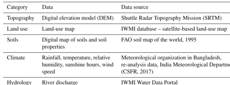
Table 1.An overview of the main data sets used in this study.

Category Data Data source

Topography Digital elevation model (DEM) Shuttle Radar Topography Mission (SRTM)

Land use Land-use map IWMI database – satellite-based land-use map

Soils Digital map of soils and soil FAO soil map of the world, 1995 properties

Climate Rainfall, temperature, relative Meteorological organization in Bangladesh, humidity, sunshine hours, wind re-analysis data, India Meteorological Department

speed (CSFR, 2017)

Hydrology River discharge IWMI Water Data Portal

of the GRB. Although this study is a theoretical exercise, it provides a scientific justification for a complete investigation (including field pilot tests) into the plausibility for a well-designed managed aquifer recharge program to enhance the sub-surface storage in the GRB.

2 Methodology 2.1 The model

Many models have been developed (e.g., Eastham et al., 2010; Gosain et al., unpublished data; World Bank, 2012) to study water issues in the Ganges River basin (Johnston and Smakhtin, 2014). However, they are not available to the public. To overcome this restriction and provide the research community with a working hydrological model for the Ganges River basin, the International Water Man-agement Institute (IWMI) has developed a publicly avail-able hydrological model for the basin (Muthuwatta et al., 2014) using the Soil and Water Assessment Tool (SWAT) (Arnold et al., 1998). The model setup files can be down-loaded from the website http://waterdata.iwmi.org/pages/ model_inventory.php and used in further applications and scenario analyses in a variety of projects.

SWAT is a widely used, semi-distributed conceptual hydrological model developed by the Agricultural Re-search Service of the United States Department of Agricul-ture (USDA) over the last 30 years, and is available free of charge as a public domain model (Arnold et al., 1998; Gassman et al., 2007; Sood et al., 2013). The model has been previously being used for number of studies for different wa-tershed scales (e.g., Muttiah and Wurbs, 2002; Ringler et al., 2010; Singh and Gosain, 2011; Sood et al., 2013). The hy-drological ability of the model to capture real-world situa-tions is extensively discussed in these articles. Broadly, the SWAT input data can be grouped into five categories: topog-raphy or terrain, land use, soil, land use management and cli-mate (Neitsch et al., 2002). SWAT possesses adequate rep-resentation of processes governing hydrology and is

particu-larly suitable for application in large river basins. In SWAT, a river basin is subdivided into a number of catchments, so that each catchment has at least one representative stream. Based on unique combinations of soil, land use and slope, the catchments were further divided into hydrological response units (HRUs), which are the fundamental units of calculation. Subdividing the watershed into areas having unique land use, soil and slope combinations enables the model to reflect dif-ferences in evapotranspiration and other hydrologic condi-tions. HRUs allow for a modeling efficiency by lumping pix-els with similar land use, soil and slope properties.

SWAT simulates the local water balance of the catchment through four storage volumes – snow, soil profile, shallow aquifer and deep aquifer – based on the soil water balance (Eq. 1):

SWt=SW0+ t

X

t=1

(Rt−SRt−ETt−Pt−Gt) , (1)

where SWt is the soil water content minus the wilting-point

water content at time t, and Rt, SRt, ETt,Pt, and Gt are

the daily amounts (in millimeters) of rainfall, runoff, evapo-transpiration, percolation and groundwater flow, respectively, at time t. SW0 is the initial soil water content. The

simu-lated processes include direct runoff (in SWAT direct runoff is termed surface runoff), infiltration, evaporation, transpi-ration, lateral flow, and percolation to shallow and deep aquifers.

2.2 The data and model setup

The model used in this study was set up using the data sets shown in Table 1. The Ganges River basin was delineated us-ing 3000 ha as the minimum area threshold and has resulted in 1684 catchments (Fig. 1). The area threshold was selected by trial and error in an attempt to represent major tributaries in GRB, while also keeping the SWAT sub-basins to a mini-mum.

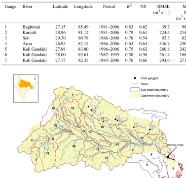
Table 2.Model performance indicators for seven locations in the GRB.

Gauge River Latitude Longitude Period R2 NS RMSE Max. (m3s−1) flow (m3s−1)

1 Baghmati 27.15 85.49 1981–2006 0.83 0.82 39.7 987.0 2 Karnali 28.96 81.12 1981–2006 0.79 0.61 224.4 2140.7 3 Seti 29.30 80.78 1986–2006 0.76 0.54 92.3 827.4 4 Arun 26.93 87.15 1986–2006 0.63 0.64 446.7 2300.6 5 Kali Gandaki 27.88 83.80 1996–2006 0.75 0.62 280.8 2420.6 6 Kali Gandaki 28.00 83.61 1987–1995 0.58 0.58 261.4 1081.9 7 Kali Gandaki 27.75 82.35 1984–2006 0.76 0.66 293.6 2710.4

Figure 1.Sub-basins and catchments of the Ganges River basin (names of the sub-basins are given in Table 3).

SWAT model developed for the Ganges does not entirely cover the areas that belong to West Bengal and Bangladesh. However, this does not affect the current study, as its focus is to assess water availability in the upstream sub-basins of the Ganges River basin.

Figure 1 shows the 22 major sub-basins (Table 3) in the GRB as defined by the Central Water Commission (CWC) of India, which is the main government agency responsible for water resource development and management in the Ganges River basin. Since the focus of this study is to estimate wa-ter availability in the sub-basins within India, Nepal is con-sidered one region. The smaller spatial units inside those 22 sub-basins and Nepal are termed “catchments” and were developed using the SWAT interface, as discussed above. The catchments do not completely match with some of the sub-basins due to limitation in SWAT in processing coastal basins.

The model was initially calibrated and validated for the monthly discharge data collated at Harding Bridge. The

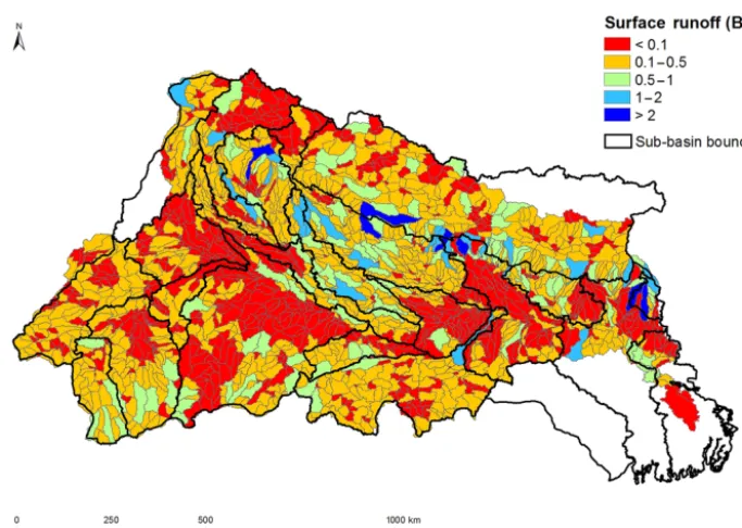
Table 3.Runoff of the sub-basins.

Number Sub-basin Share of runoff as a

Runoff (billion m3) percentage of the total

Mean Standard SR75 Wet Dry

deviation months months (June– (November– October) May)

1 Above the Ramganga confluence 10.02 5.04 5.48 81.2 18.8

2 Banas 9.89 7.11 3.51 93.8 6.2

3.4 Bangladesh – – – –

5 Bhagirathi and others – – – –

6 Chambal Lower 2.24 1.37 1.23 94.8 5.2

7 Chambal Upper 8.73 3.01 6.60 90.2 9.8

8 Damodar – – – –

9 Gandak and others 16.03 6.57 11.79 86.0 14.0

10 Ghaghara 35.56 17.55 23.34 84.0 16.0

11 Ghaghara confluence to the Gomti confluence 4.72 2.07 3.32 88.3 11.7

12 Gomti 13.64 7.34 9.75 90.8 9.2

13 Kali Sindh and others up to the confluence with Parbati 15.48 6.64 10.51 80.9 19.1

14 Kosi 9.44 3.95 6.81 72.8 27.2

15 Nepal 63.17 11.59 54.44 88.0 12.0

16 Ramganga 15.56 7.79 10.11 82.6 17.4

17 Son 19.50 7.88 14.08 85.1 14.9

18 Tons 6.75 2.47 5.17 88.5 11.5

19 Upstream of the Gomti confluence with Muzaffarnagar 9.38 4.77 5.70 87.8 12.2

20 Yamuna Lower 22.42 10.78 15.21 93.8 6.2

21 Yamuna Middle 4.81 3.70 2.14 78.7 21.3

22 Yamuna Upper 7.19 3.92 4.49 82.7 17.3

2.3 Simulating sub-basin runoff

Annual time series of catchment-scale runoff from 1991 to 2010 were constructed by aggregating daily runoff sim-ulated by SWAT. Next, using geographic information sys-tem (GIS) techniques, annual runoff time series were esti-mated for all sub-basins within the modeled area of the GRB. The study uses the hydrographs of the simulated runoff (SR) to estimate the 75 % dependable runoff (SR75). SR75 is an

estimate of the runoff that can be expected in the basin, on average, every 3 out of 4 years, and is considered to be a re-liable estimate of water availability for augmenting ground-water storage (Wang et al., 2014).

2.4 Simulating groundwater recharge scenarios in Ramganga

To examine the effect of groundwater recharge on the hydrol-ogy such as monthly river flow, the Ramganga sub-basin lo-cated in the northwestern part of the basin was selected. The Ramganga sub-basin was selected because it is the first major upstream basin with the typical water resource management challenge of managing seasonal water variability and meet-ing water demand. The area of the Ramganga sub-basin is about 32 000 km2 and it belongs to two administrative

dis-tricts: Uttaranchal and Uttara Pradesh. The important trib-utaries that flow into the Ramganga River are Kho, Gangan, Aril, Kosi, and Gorra. The surface water potential in the basin is about 18.6 billion m3. The population in the basin is about 20 million. The groundwater recharge was controlled in the SWAT model by changing the curve number (CN). The CN determines the runoff in hydrological models. Reducing the CN in the SWAT increases groundwater recharge.

2.5 Linking river flow to flood inundated areas

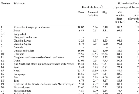
Figure 2.Mean annual runoff of the 1684 sub-basins (1991–2010).

3 Results

3.1 Runoff of the sub-basins

The spatial and temporal distribution of the annual runoff is analyzed to determine the water availability in different sub-basins. River flow includes direct runoff on surface, lat-eral flow and baseflow from groundwater, which can be cap-tured by diversion or from dams. Direct runoff is calculated in SWAT using the SCS curve number method (Soil conser-vation service, 1972). In standard hydrological definitions, it is infiltration excess overland flow, which is part of precipita-tion, that is left after infiltration. It can be captured for MAR before it reaches the stream (in this paper runoff is referred to as the direct runoff calculated by SWAT). Therefore, only the runoff portion was considered for augmenting SSS. Figure 2 shows the simulated catchment-scale mean annual runoff.

The runoff of catchments ranges from less than 0.1 billion m3 to more than 2.0 billion m3. The statistics of the estimated surface runoff for the sub-basins are given in Table 3.

The estimates of mean annual runoff at sub-basin scale range from 2.24 billion m3 in Chambal Lower (6) to 63.17 billion m3 in Nepal (15). Additionally, the high stan-dard deviations in Table 4 indicate significant temporal vari-ation within sub-basins. Further analysis shows that runoff in the wet months (June to October) is more than 80 % of the annual runoff in most sub-basins (Table 4, last two columns). This intra- and inter-annual variability of the flows clearly indicates the need for storages to capture the excess runoff during the monsoon season, which could be SSS. For this

analysis, SR75 was used to identify the sub-basins that

con-sistently produce higher volumes of runoff. Figure 3 shows the spatial distribution of the SR75of the sub-basins.

The Ghaghara (10) sub-basin and Nepal have, by far, the largest SR75. The Kali Sindh (13), Ramganga (16),

Son (17) and Yamuna Lower (20) sub-basins have more than 10 billion m3of SR75. The Gandak (9) also produces higher

runoff, but the sub-basin is located in the downstream area of the Ganges River basin. Because of the high monsoon runoff, the upstream sub-basins contribute substantially to flooding in the downstream areas of the Ganges River basin.

3.2 Total discharge of the sub-basins

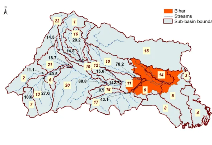
The mean annual discharge from the upstream sub-basins from 2001 to 2010 was estimated and is presented in Fig. 4.

Figure 3.Sub-basin-scale annual dependable runoff (SR75) in the Ganges River basin (1991–2010).

Figure 4.Mean annual outflow (billion m3) from the sub-basins in the Ganges River basin (the numbers in black represent the mean annual outflow, and the numbers in brown in the yellow background represent the numbers of the sub-basins).

and Ramganga are 17, 10 and 7 %, respectively. The esti-mated discharges at the sub-basin outlets, as shown in Fig. 4, include the contributions from upstream sub-basins and also the contribution of groundwater and runoff to the river flow. Therefore, the values presented in Fig. 4 are significantly higher compared to the surface values presented in Fig. 3.

3.3 Unmet water demand for agriculture

Amarasinghe et al. (2016) estimated the unmet agricultural water demand. Two scenarios were considered in the analysis (Table 4).

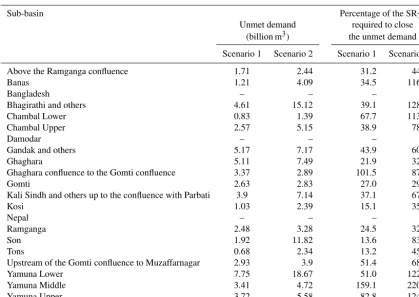
(Novem-Table 4.Sub-basin-wise unmet agricultural water demand and the percentage of runoff required to close the unmet demand.

Sub-basin Percentage of the SR75

Unmet demand required to close (billion m3) the unmet demand

Scenario 1 Scenario 2 Scenario 1 Scenario 2

Above the Ramganga confluence 1.71 2.44 31.2 44.5

Banas 1.21 4.09 34.5 116.6

Bangladesh – – – –

Bhagirathi and others 4.61 15.12 39.1 128.4

Chambal Lower 0.83 1.39 67.7 113.4

Chambal Upper 2.57 5.15 38.9 78.0

Damodar – – – –

Gandak and others 5.17 7.17 43.9 60.8

Ghaghara 5.11 7.49 21.9 32.1

Ghaghara confluence to the Gomti confluence 3.37 2.89 101.5 87.1

Gomti 2.63 2.83 27.0 29.0

Kali Sindh and others up to the confluence with Parbati 3.9 7.14 37.1 67.9

Kosi 1.03 2.39 15.1 35.1

Nepal – – – –

Ramganga 2.48 3.28 24.5 32.4

Son 1.92 11.82 13.6 83.9

Tons 0.68 2.34 13.2 45.3

Upstream of the Gomti confluence to Muzaffarnagar 2.93 3.9 51.4 68.5

Yamuna Lower 7.75 18.67 51.0 122.8

Yamuna Middle 3.41 4.72 159.1 220.2

Yamuna Upper 3.72 5.58 82.8 124.2

ber to March) from 26 million ha (current irrigated area in this season) to 30 million ha (irrigable area), and in the hot-weather season (April to June) from 3 million ha (current irrigated area in this season) to 30 million ha (ir-rigable area), respectively.

– Scenario 2: provide irrigation to the total cropped area. At present, not all cropped area is equipped for irriga-tion; i.e., irrigable area (30 million ha) is less than the cropped area (35 million ha). Therefore, scenario 2 in-creases irrigable area and inin-creases irrigated area from 26 to 35 million ha in the Rabi season and from 3 to 35 million ha in the hot-weather (April to June) season, respectively.

As of now, all the sub-basins in the Ganges River basin have substantial unmet water demand for agriculture in the dry season. Therefore, capturing a substantial portion of the runoff during the monsoon months can help close the gap be-tween current supply of water and demand in the dry months, thus increasing agricultural productivity in these sub-basins. Table 4 presents the sub-basin-wise unmet demand and the percentage of dependable runoff required to close the unmet demand.

In the sub-basins, the total unmet demands are 55.03 and 108.4 billion m3 under scenarios 1 and 2, respectively. The values presented in Table 4 show that, for some sub-basins,

annual unmet demand exceeds the annual water availability. In these sub-basins, only a part of the unmet demand can be satisfied by additional underground storage. In some other sub-basins, the unmet demand is less than 30 % of the SR75

of runoff. These sub-basins have the potential to meet all the unmet demand with SSS. In the Ramganga sub-basin, the SR75 of runoff is about 10.1 billion m3, and approximately

83 % of this runoff occurs during the wet season. To meet the maximum unmet agricultural water demand in the Ramganga sub-basin only requires one to capture 33 % of the monsoon runoff.

3.4 Effect of enhanced groundwater recharge and increased pumping on the hydrology

im-Table 5.Mean monthly distribution of river flow and baseflow in the Ramganga sub-basin under different groundwater recharge and abstrac-tion scenarios (BL – baseline scenario; S-35 – 35 % increase in groundwater recharge; S-65 – 65 % increase in groundwater recharge).

Month Baseflow Additional Baseflow Baseflow

(groundwater recharge water additional irrigation additional irrigation Flow scenarios) requirement scenarios S-35 scenarios S-65

C1 C2 C3 C4 C5 C6 C7 C8 C9 C10 C11 C12 C13

BL S-35 S-65 BL S-35 S-65 100 % 60 % 50 % 100 % 70 % 60 %

Jan 0.24 0.23 0.25 0.16 0.25 0.29 0.27 0.02 0.09 0.11 0.02 0.10 0.13 Feb 0.33 0.28 0.25 0.14 0.23 0.27 0.17 0.07 0.13 0.15 0.10 0.15 0.17 Mar 0.24 0.23 0.24 0.20 0.24 0.29 0.03 0.20 0.22 0.22 0.25 0.26 0.27 Apr 0.12 0.13 0.15 0.17 0.17 0.24 0.17 0.17 0.18 0.20 0.20 0.27 May 0.06 0.07 0.07 0.10 0.11 0.13 0.09 0.10 0.10 0.11 0.11 0.11 Jun 0.87 0.66 0.51 0.05 0.06 0.10 0.06 0.07 0.07 0.08 0.08 0.08 Jul 4.02 3.40 2.90 0.43 0.54 0.80 0.39 0.44 0.45 0.80 0.79 0.79 Aug 6.00 5.51 5.12 1.47 2.07 2.57 2.07 2.07 2.07 2.57 2.57 2.57 Sep 5.33 5.38 5.43 2.24 3.07 3.77 3.07 3.07 3.07 3.77 3.77 3.77 Oct 2.01 2.55 2.99 1.97 2.67 3.25 2.67 2.67 2.67 3.25 3.25 3.25 Nov 0.91 1.23 1.48 1.03 1.39 1.79 0.13 1.26 1.31 1.32 1.66 1.70 1.71 Dec 0.41 0.54 0.64 0.45 0.62 0.97 0.23 0.39 0.48 0.51 0.74 0.81 0.83

Total 20.54 20.20 20.02 8.42 11.41 14.45 0.83 10.46 10.82 10.92 13.55 13.79 13.95

plemented in the SWAT model by removing water from the groundwater storage. The groundwater pumped is assumed to be consumptive use for ET and hence is lost from the system. In Amarasinghe et al. (2016), scenario 2 of unmet agriculture water demand indicated that the agricultural ar-eas in the Ramganga sub-basin could be incrar-eased by an-other 160 000 ha. Thus for this analysis we only consider scenario 2 (from Amarasinghe et al., 2016) of the unmet agri-culture water demand. We assume that the additional agricul-ture area will be wheat, as this crop is predominantly grown during the period of November to March. To estimate wa-ter requirements for additional wheat areas from Novem-ber to March, crop coefficients (kc) for wheat as obtained

from FAO56 (Allen et al., 1998) for similar climatic condi-tions and crop development stages were used. The Penman– Monteith method served to estimate the daily reference evap-otranspiration (ET0) as required for the crop water

require-ment estimations. Estimated water requirerequire-ment for wheat was calculated as 520 mm, which is within the range of rec-ommended water requirements (450–650 mm) for regions with similar settings (see Doorenbos and Kassam, 1979).

Table 5 shows the effect of enhanced groundwater recharge and increased pumping on the baseflow and to-tal streamflow at the main outlet of Ramganga (billion m3). Columns 1–3 (c1 to c3) present the total streamflow at the main outlet of the Ramganga sub-basin under baseline (BL), S-35 and S-65 scenarios, respectively. Columns 4 to 6 show the simulated monthly baseflow under the three scenarios. Additional water required to expand the irrigated wheat area of 160 000 ha during the period November to March is pre-sented in column 7. The effect of additional pumping under

S-35 and S-65 is presented in columns 8 to 13. Column 8 shows the monthly baseflow if 100 % of the additional area is irrigated by groundwater under the S-35 scenario, while val-ues in columns 9 and 10 are estimated by assuming 60 and 50 % of the 160 000 ha irrigated. Columns 11–13 present the monthly baseflow under S-65 and assume 100, 70 and 60 % of the 160 000 ha irrigated by groundwater, respectively.

Under S-35 scenarios, irrigating 100 % of the additional area would result in reduction of baseflow below the BL sce-nario during December to February. However, as presented in Table 5, for scenario S-35, additional irrigation to cover 50 % of the new wheat area would still maintain the baseflow above the BL level other than in January. Irrigating 60 % of additional irrigated wheat areas would reduce the baseflow volumes below the BL levels in January and February. Re-sults, further, indicate that under the S-65 scenario it will be possible to supply irrigation to 70 % of the additional irri-gated area without reducing the volumes of baseflow simu-lated in the BL scenario. When it is 70 % of the additional irrigated area, baseflow will reduce by a negligible amount in January.

When water balance is considered, the summation of to-tal baseflow under abstraction scenarios and additional water requirement must be equal to the total baseflow under a no pumping scenario. For instance, the sum of the totals of C8 and C7 must be equal to the total of the C5 column. However, we found some differences which are negligible. In this case, the error is about 0.12, which is about 1.05 % compared to the total baseflow presented in C5. The water balance errors un-der the remaining five abstraction scenarios also range from 0.0 to 0.8 %. We presume that these small differences are due to changes in other hydrological process such as changes in soil moisture and evapotranspiration as a result of increased groundwater infiltration.

3.5 Effect on floods

The relationship between the simulated maximum monthly river flow and the maximum flood inundated areas in Ram-ganga is shown in Fig. 5. The horizontal axis represents simulated maximum monthly river flow during each year from 2003 to 2010 at the Ramganga outlet. The vertical axis shows the maximum flood inundation areas estimated based on the satellite images in the corresponding year (Amarnath et al., 2012).

The coefficient of the determinant (R2) indicates a strong correlation between the area under floods and the annual runoff, and this implies that the maximum monthly runoff explains more than 70 % of the variation in maximum flood inundated area. The mathematical relationship between max-imum flood inundated area and the runoff is given in Eq. (2): Maximum flood inundated area=568.7×ln(Flow)−356.2. (2) The maximum monthly flow in Ramganga of about 6.0 billion m3in August (Table 5) has a corresponding flood inundated area of about 660 km2. Reduction of peak flow to 5.5 billion m3 (35 % groundwater recharge scenario) would reduce the flood inundated area by about 6.9 %. Similarly, the reduction of flood inundated areas compared to the baseline scenario is about 13.0 % for the 65 % groundwater recharge scenario. For this scenario, the reduced outflow (in August) from the basin is about 15 %. This analysis shows the

poten-Figure 5.Relationship between annual maximum flood inundated area and the maximum monthly river flow in Ramganga.

tial impacts of enhanced sub-surface storage on the flooding in the Ramganga sub-basin located in the upstream. The vol-ume of inflow in the Ramganga is negligible compared to the inflow received by the areas such as Bihar in the down-stream. Therefore, to understand the potential impacts of SSS on flooding in the GRB, further research is required to inves-tigate the effect of SSS on control of floods in the down-stream areas.

4 Discussion

Water availability and demand analysis conducted in the Ganges River basin show that there is a substantial mis-match between water demand and supply. For instance, es-timated unmet annual water demand for agriculture in the GRB (based on the two scenarios discussed above) ranges from 55.03 to 108.4 billion m3, while annual total runoff gen-erated in the basin is about 298±99 billion m3, of which 80 % occurs during the monsoon months. In this situation, strategies must be formulated to manage available water in the GRB in a more productive manner. One management op-tion discussed in this paper is using SSS. Augmenting SSS is important in securing downstream water availability for ecosystems and other uses such as agricultural, domestic and industrial.

soil moisture could have made the model more robust, but such data do not exist (although satellite products are there). Results of the SWAT model demonstrate its capability in estimating the spatial and temporal water availability in the sub-basins of the GRB and in assessing the effect of aug-menting SSS on the hydrology of the basin. In all the sce-narios, augmenting SSS does not show much difference in total annual flow from Ramganga, but there are intra-year changes. There is reduction in flow during the peak season but an increase in flow during the dry season. This indicates that augmenting SSS can help in flood reduction while im-proving water availability for crops in the dry season. For the excess irrigation scenarios considered, 80 000 to 112 000 ha of additional agriculture land can be irrigated by groundwa-ter without affecting the baseflow in the basin. There still remain some limitations in this study, mainly due to the lim-itations with the model such as unavailability of the model in handling of groundwater depth and no detailed linkages between surface water and groundwater (since SWAT is pre-dominantly a surface water model).

Flood inundated areas based on satellite remote sensing data (provided by another study) allowed us to investigate the impact of SSS on downstream floods. However, the re-lationship established between flood inundated areas and the river flow was only for Ramganga, and further investigations are required to understand how SSS will impact large floods in the downstream part of the basin.

5 Conclusions

Creating additional SSS beyond the current levels in the Ganges River basin can simultaneously enhance water sup-ply and control downstream floods. The sub-basin-wise mean annual runoff ranges from 2.24 to 35.56 billion m3, and the contribution of runoff from Nepal is about 63 billion m3. Several sub-basins in the Ganges River basin produce suf-ficiently high dependable annual runoff that can be stored underground and used during the dry season. For instance, annual runoff in each of the five sub-basins in the upstream of the Ganges River basin is more than 10 billion m3, which is about 30 % of total runoff generated in the GRB. Compari-son of sub-basin-wise runoff with the estimated unmet water demand indicates that capturing only a portion of the wet-season runoff would be sufficient to provide water to irrigate all the irrigable land in the dry months. Sub-basin-wise river flow analysis in the GRB shows that approximately 30 % of the upstream flow to Bihar comes through the Ghaghara and Yamuna Lower sub-basins. This runoff contributes to the re-current floods in Bihar.

A case study based on Ramganga indicates that increasing 35 and 65 % groundwater recharge compared to the baseline scenario may reduce the peak monthly flow by about 6.8 and 12.3 %, respectively. Further, the results indicate that the dry season flow (October to May) can increase by 21 and 40 % in

these two scenarios before meeting unmet demand by pump-ing.

More than 70 % of the variations of flood inundated areas in the Ramganga sub-basin can be explained by the maxi-mum monthly river flow values. By increasing groundwater recharge by 35 and 65 % during the peak flow months the flood inundated area can be reduced by about 6.6 and 8 %, respectively.

This study focused on spatio-temporal water availability and the impacts of SSS on the hydrology in the GRB. Pump-ing scenarios simulated by the SWAT model indicated that additional wheat areas in the Rabi season could be irrigated by the increased SSS under a 35 % increase in groundwater recharge and a 65 % increase in groundwater recharge sce-narios.

This study only discusses the surface water availability for SSS, without going into details regarding suitability of recharge areas. A detailed analysis of the soil, topographic and geological characteristics is required to determine the suitable areas for groundwater recharge.

Data availability. Sources of the data used in this study are shown in Table 1. The SWAT model setup files can be found from the web-site: http://waterdata.iwmi.org/pages/model_inventory.php.

Part of the daily meteorological data sets used here were ob-tained from Indian Meteorological Department (IMD) and are not available to the public as far as the authors know. Therefore, the authors cannot provide them. The other meteorological data were downloaded from The National Centers for Environmental Pre-diction (NCEP) HYPERLINK http://rda.ucar.edu/pub/cfsr.html Cli-mate Forecast System Reanalysis (CFSR). This data set is freely available https://globalweather.tamu.edu/ (CSFR, 2017).

Competing interests. The authors declare that they have no conflict of interest.

Acknowledgements. This research study was undertaken as part of the CGIAR Research Program on Water, Land and Ecosystems (WLE) by the International Water Management Institute (IWMI), Colombo, Sri Lanka, and the National Institute of Hydrology (NIH), Roorkee, India. The authors would like to acknowledge the satellite data provided by the IWMI’s senior researcher, Giriraj Amarnath, for flood inundation areas in the study area. Authors thank the two anonymous reviewers and Nanditha Basu for their useful comments and suggestions during the review process.

Edited by: N. Basu

References

Allen, R. G., Pereira, L. S., Raes, D., and Smith, M.: Crop evapo-transpiration: guidelines for computing crop water requirements, FAO irrigation and drainage paper 56, FAO, Rome, 300 pp., 1999.

Amarasinghe, U. A., Muthuwatta, L., Surinaidu, L., Anand, S., and Jain, S. K.: Reviving the Ganges Water Machine: potential, Hy-drol. Earth Syst. Sci., 20, 1085–1101, doi:10.5194/hess-20-1085-2016, 2016.

Amarnath, G., Ameer, M., Aggarwal, P., and Smakhtin, V.: Detect-ing spatio-temporal changes in the extent of seasonal and annual flooding in South Asia using multi-resolution satellite data, Proc. SPIE, 8538, 853818, doi:10.1117/12.974653, 2012.

Arnold, J. G., Srinivasan, R., Muttiah, R. S., and Williams, J. R.: Large area hydrologic modeling and assessment part 1: Model development, J. Am. Water Resour. Assoc., 34, 73–89, 1998. Bouwer, H.: Integrated water management: Emerging issues and

challenges, Agr. Water Manage., 45, 217–228, 2000.

Chinnasamy, P.: Depleting groundwater – an opportunity for flood storage? A case study from part of the Ganges River basin, India, Hydrol. Res., 48, 431–441 doi:10.2166/nh.2016.261, 2016 CSFR (Climate Forecast System Reanalysis): National Centers

for Environmental Prediction, available at: https://globalweather. tamu.edu/, last access: 22 May 2017.

Dillon, P. J.: Future management of aquifer recharge, Hydrogeol. J., 13, 313–316, 2005.

Doorenbos, J. and Kassam, A. H.: Yield response to water, Irriga-tion and drainage paper 33, FAO, Rome, Italy, 1979.

Eastham, J., Kirby, M., Mainuddin, M., and Thomas, M.: Water use accounts in CPWF basins: Simple water-use accounting of the Ganges Basin, CPWF Working Paper: Basin Focal Paper series BFP05, CGIAR Challenge Program on Water and Food, Colombo, Sri Lanka, p. 30, 2010.

Gassman, P. W., Reyes, M. R., Green, C. H., and Arnold, J. G.: The soil water assessment tool: Historical development, applications, and future research directions, T. ASABE, 50, 1211–1250, 2007. Ghayoumian, J., Mohseni Saravi, M., Feiznia, S., Nouri, B., and Malekian, A.: Application of GIS techniques to determine ar-eas most suitable for artificial groundwater recharge in a coastal aquifer in southern Iran, J. Asian Earth Sci., 30, 364–374, 2007. Gosain, A. K. and Sirinivasan, R.: Water system modeling for

Ganges basin, World bank, New Delhi, 2011.

Huda, A. and Shamsul, T. M.: Constraints and opportunities for cooperation towards development of water resources in the Ganges basin, in: Sustainable Development of the Ganges– Brahmaputra–Meghna Basins, edited by: Biswas, A. K. and Uitto, J. I., United Nations University Press, Tokyo, Japan, 46– 57, 2001.

Johnston, R. and Smakhtin, V.: Hydrological modeling of large river basins: How much is enough?, Water Resour. Manage., 28, 2695–2730, doi:10.1007/s11269-014-0637-8, 2014.

Khan, M. R., Voss, C. I., Yu, W., and Michael, H. A.: Water re-sources management in the Ganges Basin: A comparison of three strategies for conjunctive use of groundwater and surface water, Water Resour. Manage., 28, 1235–1250, doi:10.1007/s11269-014-0537-y, 2014.

Ministry of water resources: Ganges Basin Report, version 2, Gov-ernment of India, 2014.

Mishra, D. K.: The Bihar flood story, Econ. Polit. Week., 32, 2206– 2217, 1997.

Morrow, E., Mitrovica, J., and Fotopoulos, G.: Water storage, net precipitation, and evapotranspiration in the Mackenzie River Basin from october 2002 to september 2009 inferred from GRACE satellite gravity data, J. Hydrometeorol., 12, 467–473, 2011.

Muthuwatta, L. P., Sood, A., and Sharma, B.: Model to assess the impacts of external drivers on the hydrology of the Ganges River Basin, IAHS Publ., 364, 76–81, 2014.

Muttiah, R. S. and Wurbs, R. A.: Modeling the impacts of climate change on water supply reliabilities, Water Int., 27, 407–419, 2002.

Neitsch, S. L., Arnold, J. G., Kiniry, J. R., Williams, J. R., and King, K. W.: Soil and water assessment tool theoretical documentation, version 2000, Grassland, Soil and Water Research Laboratory, Temple, TX, and Blackland Research Center, Temple, TX, 2002. Onta, I. R.: Harnessing the Himalayan waters of Nepal: A case for partnership for the Ganges basin, in: Sustainable development of the Ganges–Brahmaputra–Meghna basins, UNU Press, Tokyo, 100–121, 2001.

Pavelic, P., Srisuk, K., Saraphirom, P., Nadee, S., Pholkern, K., Chusanathas, S., Munyou, S., Tangsutthinon, I., and Smakhtin, V.: Balancing-out floods and droughts: Opportunities to utilize floodwater harvesting and groundwater storage for agricultural development in Thailand, J. Hydrol., 470–471, 55–64, 2012. Revelle, R. and Lakshminarayana, V.: The Ganges water machine,

Science, 188, 611–616, 1975.

Ringler, C., Caib, X., Wang, J., Ahmed, A., Xue, Y., Xu, Z., and You, L.: Yellow River basin: Living with scarcity, Water Int., 35, 681–701, 2010.

Rodell, M., Velicogna, I., and Famiglietti, J. S.: Satellite-based esti-mates of groundwater depletion in India, Nature, 460, 999–1002, 2009.

Sadoff, C., Harshadeep, N. R., Blackmor, D., Wu, X., O’Donnell, A., Jeuland, M., Lee, S., and Whittington, D.: Ten fundamental questions for water resources development in the Ganges: Myths and realities, Water Policy, 15, 147–164, 2013.

Sharma, B. R. and de Condappa, D.: Opportunities for harnessing the increased contribution of glacier and snowmelt flows in the Ganges basin, Water Policy, 15, 9–25, 2013.

Singh, A. and Gosain, A. K.: Climate-change impact assessment using GIS-based hydrological modelling, Water Int., 36, 386– 397, 2011.

SMEC – Snow Mountain Engineering Corporation International Pty Ltd, Preparation of Ghanga Gomti Basin plans and development of decision support systems, Final Report prepared for the State Water Resources Agency, Uttar Pradesh, 2009.

Soil conservation service: section 4, Hydrology in National Engi-neering hand book, University of Minnesota, 1972.

Sood, A., Muthuwatta, L., and McCartney, M.: A SWAT evaluation of the effect of climate change on the hydrol-ogy of the Volta River basin, Water Int., 38, 297–311, doi:10.1080/02508060.2013.792404, 2013.

Swenson, S. and Wahr, J.: Post-processing removal of corre-lated errors in GRACE data, Geophys. Res. Lett., 33, L08402, doi:10.1029/2005GL025285, 2006.

World Bank: Ganges strategic basin assessment: A discussion of regional opportunities and risks, Draft final report, March 2012, World Bank, Washington, 2012.