Assessment of precipitation and temperature data from CMIP3 global climate models for hydrologic simulation

www.hydrol-earth-syst-sci.net/19/361/2015/ doi:10.5194/hess-19-361-2015

© Author(s) 2015. CC Attribution 3.0 License.

Assessment of precipitation and temperature data from CMIP3

global climate models for hydrologic simulation

T. A. McMahon1, M. C. Peel1, and D. J. Karoly2

1_{Department of Infrastructure Engineering, University of Melbourne, Victoria, 3010, Australia}

2_{School of Earth Sciences and ARC Centre of Excellence for Climate System Science, University of Melbourne,} Victoria, 3010, Australia

Correspondence to: M. C. Peel ([email protected])

Received: 25 March 2014 – Published in Hydrol. Earth Syst. Sci. Discuss.: 5 May 2014 Revised: 8 December 2014 – Accepted: 9 December 2014 – Published: 21 January 2015

Abstract. The objective of this paper is to identify better

performing Coupled Model Intercomparison Project phase 3 (CMIP3) global climate models (GCMs) that reproduce grid-scale climatological statistics of observed precipitation and temperature for input to hydrologic simulation over global land regions. Current assessments are aimed mainly at exam-ining the performance of GCMs from a climatology perspec-tive and not from a hydrology standpoint. The performance of each GCM in reproducing the precipitation and tempera-ture statistics was ranked and better performing GCMs iden-tified for later analyses. Observed global land surface precip-itation and temperature data were drawn from the Climatic Research Unit (CRU) 3.10 gridded data set and re-sampled to the resolution of each GCM for comparison. Observed and GCM-based estimates of mean and standard deviation of an-nual precipitation, mean anan-nual temperature, mean monthly precipitation and temperature and Köppen–Geiger climate type were compared. The main metrics for assessing GCM performance were the Nash–Sutcliffe efficiency (NSE) index and root mean square error (RMSE) between modelled and observed long-term statistics. This information combined with a literature review of the performance of the CMIP3 models identified the following better performing GCMs from a hydrologic perspective: HadCM3 (Hadley Centre for Climate Prediction and Research), MIROCm (Model for In-terdisciplinary Research on Climate) (Center for Climate System Research (The University of Tokyo), National Insti-tute for Environmental Studies, and Frontier Research Cen-ter for Global Change), MIUB (Meteorological Institute of the University of Bonn, Meteorological Research Institute of KMA, and Model and Data group), MPI (Max Planck

Insti-tute for Meteorology) and MRI (Japan Meteorological Re-search Institute). The future response of these GCMs was found to be representative of the 44 GCM ensemble mem-bers which confirms that the selected GCMs are reasonably representative of the range of future GCM projections.

1 Introduction

Our primary objective in this paper is to identify better per-forming GCMs from a hydrologic perspective. To do this we assess how well 22 global climate models (GCMs) from the World Climate Research Programme’s (WCRP) Cou-pled Model Intercomparison Project phase 3 (CMIP3) multi-model data set (Meehl et al., 2007) are able to reproduce GCM grid-scale climatological statistics of observed precip-itation and temperature over global land regions. We recog-nise that GCMs model different variables with a range of success and that no single model is best for all variables and/or for all regions (Lambert and Boer, 2001; Gleckler et al., 2008). The approach adopted here is not inconsistent with Dessai et al. (2005) who regarded the first step in evaluat-ing GCM projection skill is to assess how well observed cli-matology is simulated. We also recognise there have been assessments published in peer-reviewed journals, but all ap-pear to be assessed from a climate science perspective. This review concentrates on GCM variables and statistical tech-niques that are relevant to engineering hydrologic practice.

pro-duce long-term mean annual statistics that are broadly simi-lar to observed conditions across a wide range of locations. Here, the assessment of CMIP3 GCMs is made by compar-ing their long-term mean annual precipitation (MAP), stan-dard deviation of annual precipitation (SDP), mean annual temperature (MAT), mean monthly patterns of precipitation and temperature and Köppen–Geiger climate type (Peel et al., 2007) with concurrent observed data for 616 to 11 886 terrestrial grid cells worldwide (the number of grid cells de-pends on the resolution of the GCM under consideration). These variables were chosen to assess GCM performance because they provide insight into the mean annual, inter-annual variability and seasonality of precipitation and tem-perature, which are sufficient to estimate the mean and vari-ability of annual runoff from a traditional monthly rainfall– runoff model (Chiew and McMahon, 2002) or from a top– down annual rainfall–runoff model (McMahon et al., 2011) for hydrologic simulation purposes.

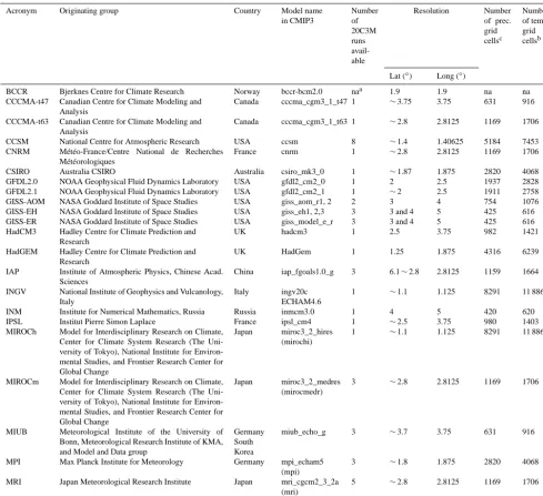
The GCMs included in this assessment are detailed in Ta-ble 1 (model acronyms adopted are listed in the taTa-ble). Al-though no quantitative assessment of the BCCR (Bjerknes Centre for Climate Research) model is made, this model is included in Table 1 as details of its performance are available in the literature which is discussed in Sect. 2. Other details in the table include the originating group for model devel-opment, country of origin, model name given in the CMIP3 documentation (Meehl et al., 2007), the number of 20C3M runs available for analysis, the model resolution and the num-ber of terrestrial grid cells used in the precipitation and tem-perature comparisons.

Readers should note that when this project began as a com-ponent of a larger study in 2010, runs from the CMIP5 were not available. We are of the view that the approach adopted here is equally applicable to evaluating CMIP5 runs for hy-drologic simulations. Conclusions about better performing models drawn from this analysis may prove similar to a comparable analysis of CMIP5 runs since most models in CMIP5 are, according to Knutti et al. (2013), “strongly tied to their predecessors”. Analysis of the CMIP5 models indi-cates that the CMIP3 simulations are of comparable quality to the CMIP5 simulations for temperature and precipitation at regional scales (Flato et al., 2013).

This study is part of a larger research project that seeks to enhance our understanding of the uncertainty of future an-nual river flows worldwide through catchment-scale hydro-logic simulation, leading to more informed decision-making for the sustainable management of scarce water resources, nationally and internationally. To achieve this, it is necessary to determine, as a minimum, how the mean and variability of annual streamflows will be affected by climate change. Other factors of less importance are changes in the auto-correlation of annual streamflow, changes in net evaporation from reservoir water surfaces and changes in monthly flow patterns, with the latter being more important for relatively small reservoirs. In this paper we deal with the key drivers of

streamflow production, namely the mean and the standard de-viation of annual precipitation and mean annual temperature, the latter is adopted here as a surrogate for potential evapo-transpiration (PET), along with secondary factors, the mean monthly patterns of precipitation and temperature. Adopting temperature as a surrogate for PET is contentious. We pro-vide a detailed discussion of this issue in the Supplementary Material associated with this paper. Suffice to say that a more complex PET formulation requires additional GCM variables other than temperature which are less reliable. This simplic-ity comes at the expense of potentially inadequate represen-tation of future changes in PET, which may have important negative consequences when modelling streamflow in energy limited catchments. Nevertheless, in the following discus-sion we concentrate on mean annual temperature as the GCM variable representing PET.

Computer models of most water resource systems that rely on surface reservoirs to offset streamflow variability adopt a monthly time step to ensure that seasonal patterns in demand and reservoir inflows are adequately accounted for. However, in a climate change scenario it is more likely that an absolute change in streamflow will have a greater impact on system yield than shifts in the monthly inflow or demand patterns. This will certainly be the case for reservoirs that operate as carryover systems rather than as within-year systems (for an explanation see McMahon and Adeloye, 2005). Therefore, in this paper we assess the GCMs in terms of annual precipita-tion and annual temperature, and patterns of mean monthly precipitation and temperature.

Following this introduction we describe, and summarise in the next section, several previous assessments of CMIP3 GCM performance. We also include some general comments on GCM assessment procedures. In Sect.3, data (observed and GCM based) used in the analysis are described. Details and results of the subsequent analyses comparing GCM esti-mates of present climate mean and standard deviation of an-nual precipitation, mean anan-nual temperature, mean monthly precipitation and temperature patterns and Köppen–Geiger climate type against observed data are set out in Sect. 4. In Sect. 5, we review the results and compare the literature in-formation with our assessments of the GCMs. The final sec-tion of the paper presents several conclusions.

2 Literature

Table 1. Details of 23 GCMs considered in this paper.

Acronym Originating group Country Model name

in CMIP3

Number of 20C3M runs avail-able

Resolution Number

of prec. grid cellsc

Number of temp. grid cellsb

Lat (◦_{) Long (}◦₎

BCCR Bjerknes Centre for Climate Research Norway bccr-bcm2.0 naa 1.9 1.9 na na

CCCMA-t47 Canadian Centre for Climate Modeling and

Analysis

Canada cccma_cgm3_1_t47 1 ∼3.75 3.75 631 916

CCCMA-t63 Canadian Centre for Climate Modeling and

Analysis

Canada cccma_cgm3_1_t63 1 ∼2.8 2.8125 1169 1706

CCSM National Centre for Atmospheric Research USA ccsm 8 ∼1.4 1.40625 5184 7453

CNRM Météo-France/Centre National de Recherches

Météorologiques

France cnrm 1 ∼2.8 2.8125 1169 1706

CSIRO Australia CSIRO Australia csiro_mk3_0 1 ∼1.87 1.875 2820 4068

GFDL2.0 NOAA Geophysical Fluid Dynamics Laboratory USA gfdl2_cm2_0 1 2 2.5 1937 2828

GFDL2.1 NOAA Geophysical Fluid Dynamics Laboratory USA gfdl2_cm2_1 1 ∼2 2.5 1911 2758

GISS-AOM NASA Goddard Institute of Space Studies USA giss_aom_r1, 2 2 3 4 754 1076

GISS-EH NASA Goddard Institute of Space Studies USA giss_eh1, 2,3 3 3 and 4 5 425 616

GISS-ER NASA Goddard Institute of Space Studies USA giss_model_e_r 3 3 and 4 5 425 616

HadCM3 Hadley Centre for Climate Prediction and

Research

UK hadcm3 1 2.5 3.75 982 1421

HadGEM Hadley Centre for Climate Prediction and

Research

UK HadGem 1 1.25 1.875 4316 6239

IAP Institute of Atmospheric Physics, Chinese Acad.

Sciences

China iap_fgoals1.0_g 3 6.1∼2.8 2.8125 1159 1664

INGV National Institute of Geophysics and Vulcanology,

Italy

Italy ingv20c

ECHAM4.6

1 ∼1.1 1.125 8291 11 886

INM Institute for Numerical Mathematics, Russia Russia inmcm3.0 1 4 5 420 620

IPSL Institut Pierre Simon Laplace France ipsl_cm4 1 ∼2.5 3.75 980 1403

MIROCh Model for Interdisciplinary Research on Climate,

Center for Climate System Research (The Uni-versity of Tokyo), National Institute for Environ-mental Studies, and Frontier Research Center for Global Change

Japan miroc3_2_hires

(mirochi)

1 ∼1.1 1.125 8291 11 886

MIROCm Model for Interdisciplinary Research on Climate,

Center for Climate System Research (The Uni-versity of Tokyo), National Institute for Environ-mental Studies, and Frontier Research Center for Global Change

Japan miroc3_2_medres

(mirocmedr)

3 ∼2.8 2.8125 1169 1706

MIUB Meteorological Institute of the University of

Bonn, Meteorological Research Institute of KMA, and Model and Data group

Germany South Korea

miub_echo_g 3 ∼3.7 3.75 631 916

MPI Max Planck Institute for Meteorology Germany mpi_echam5

(mpi)

3 ∼1.8 1.875 2820 4068

MRI Japan Meteorological Research Institute Japan mri_cgcm2_3_2a

(mri)

5 ∼2.8 2.8125 1169 1706

PCM National Center for Atmospheric Research USA pcm 1 ∼2.8 2.8125 1169 1706

a_{na: not available.}b_{Based on mean annual temperature comparison between GCM and CRU.}c_{Based on mean annual precipitation comparison between GCM and CRU.}

2.1 Procedures to assess GCM performance

Ever since the first GCM was developed by Phillips (1956) (see Xu, 1999), attempts have been made to assess the ade-quacy of GCM modelling. Initially, these evaluations were simple side-by-side comparisons of individual monthly or seasonal means or multi-year averages (Chervin, 1981). To assess model performance, Chervin (1981) extended the evaluation procedure by examining statistically the agree-ment or otherwise of the ensemble average and standard de-viation between the GCM modelled climate and the observed data using the vertical transient heat flux in an example appli-cation. Legates and Willmott (1992) compared observed with

Murphy et al. (2004). Whetton et al. (2005) introduced a demerit point system in which GCMs were rejected when a specified threshold was exceeded. Min and Hense (2006) in-troduced a Bayesian approach to evaluate GCMs and argued that a skill-weighted average with Bayes factors is more in-formative than moments estimated by conventional statistics. Shukla et al. (2006) suggested that differences in observed and GCM simulated variables should be examined in terms of their probability distributions rather than individual mo-ments. They proposed the differences could be examined us-ing relative entropy. Perkins et al. (2007) also claimed that assessing the performance of a GCM through a probability density function (PDF) rather than using the first or a sec-ond moment would provide more confidence in model as-sessment. To compare the reliability of variables (in time and space) rather than individual models, Johnson and Sharma (2009a, b) developed the variable convergence score which is used to rank a variable based on the ensemble coefficient of variation. They observed the variables with the highest scores were pressure, temperature and humidity. Reichler and Kim (2008) introduced a model performance index by first esti-mating a normalised error variance based on the square of the grid-point differences between simulated (interpolated to the observational grid) and the observed annual climate weighted and standardised with respect to the variance of the annual observations. The error variance was scaled by the average error found in the reference models and, finally, averaged over all climates.

It is clear from this brief review that no one procedure has been universally accepted to assess GCM performance, which is consistent with the observations of Räisänen (2007). We also note the comments of Smith and Chandler (2010, p. 379) who said “It is fair to say that any measure of per-formance can be subjective, simply because it will tend to reflect the priorities of the person conducting the assessment. When different studies yield different measures of perfor-mance, this can be a problem when deciding on how to in-terpret a range of results in a different context. On the other hand, there is evidence that some models consistently per-form poorly, irrespective of the type of assessment. This would tend to indicate that these model results suffer from fundamental errors which render them inappropriate.”

In 1992, Legates and Willmott (1992) assessed the ade-quacy of GCMs based mainly on January and July precipi-tation fields. Although a number of GCM assessments were carried out during the following one and a half decades, it was not until 2008 that mean precipitation, either absolute or bias, was included in GCM published assessments. In that year, Reichler and Kim (2008, p. 303) argued that the mean bias is an important component of model error.

In Table 2a and b we summarize the application of the numerical metrics and the ranking metrics of precipitation and temperature respectively applied to CMIP3 data sets at the global or country scales. These references cover the pe-riod from 2006 to 2014. Across these 15 papers, we observe

that for precipitation and temperature the spatial root mean square error, either using raw data (root mean square error – RMSE) or normalised data as a percentage of the mean value (RRMSE), is adopted in 7 of the 15 studies. (The data are normalised by the corresponding standard deviation of the reference or observed data.) This spatial root mean square metric, as well as the bias in the mean of the data, is relevant to hydrologists as it provides an indication of the uncertainty in the climate variables of interest to them. Of more rele-vance to hydrologists is the uncertainty in temporal mean and variance of climatic variables, which for precipitation are only reported in 4 of the 15 studies. Although spatial correlation is not used directly in general hydrologic inves-tigations, in GCM assessments it is often combined with the variance and spatial RMSE through the Taylor diagram (Tay-lor, 2001) which is an excellent summary of the performance of a GCM projected variable. As noted in Table 2, three pa-pers utilise this approach. Lambert and Boer (2001, p. 89) ex-tended the Taylor diagram to display the relative mean square differences, the pattern correlations and the ratio of variances for modelled and observed data. This approach to displaying the second-order statistics appears not to have been widely adopted. It is noted in Table 2a that only four papers include the mean or bias of the raw precipitation data in the GCM as-sessments which is important from a hydrologic perspective. The second set of metrics listed in Table 2b is used essentially for ranking GCMs by performance. Several other assessment tools not included in Table 2b are the climate prediction in-dex (Murphy et al., 2004) and Bayesian approaches (Min and Hense, 2006).

Specific climate features like the preservation of the ENSO (El Niño–Southern Oscillation) signal (van Oldenborgh et al., 2005) would also be considered to be a non-numerical measure of GCM performance, but in some regions to be no less important to hydrologists than the numerical mea-sures. Most of these ranking metrics have been developed for specific purposes with respect to GCMs and several have little utility for the practicing hydrologist who is primarily interested in bias, variance and uncertainty in projected es-timates of precipitation and temperature (plus net radiation, wind speed and humidity to derive potential ET) as input to drive stand-alone global and catchment hydrologic models.

2.2 Results of CMIP3 GCMs assessments

T able 2a. Numerical measures of performance assessment of CMIP3 GCMs. Reference Global, country , lar ge re gion GCMs Precipitation T emperature Reference data sets Mean of ra w data Bias in mean of ra w data V ariance of ra w data RMS or similar metric Spat. correl. T aylor plots Reference data sets Mean of ra w data Bias in mean of ra w data RMS or similar metric Spat. correl. T aylor plots Bonsal and Pro wse (2006) Northern Canada 7 GCMs CR U and other data yes yes (abs) yes yes (abs) Suppiah et al. (2007) Australia 23 GCMs Bureau of M et., Australia yes (abs) ∧ yes Bureau of Met., Australia yes yes Räisänen (2007) Global 21 GCMs CR U, GPC Pv2

yes as figure yes as figure

yes yes CR U TS2.0, NCEP-NCAR

yes as figure yes (abs) yes Gleckler et al. (2008) Global 22 GCMs GPCP/ CMAP yes (norm)# yes (norm) ERA40/NCEP- NCAR yes (norm) yes (norm) Reifen and T oumi (2009) Global 17 GCMs HadCR UT3 5 ◦× 5 ◦ yes (abs) Knutti et al. (2010) Global 23 GCMs ERA40 yes yes (abs) yes Macadam et al. (2010) Global 17 GCMs HadCR UT3 data set

yes as figure*

Hagemann

et

al.

(2011)

Global

MPI CNRM IPSL WFD (ERA-40) yes as

figure

yes as figure yes as figure

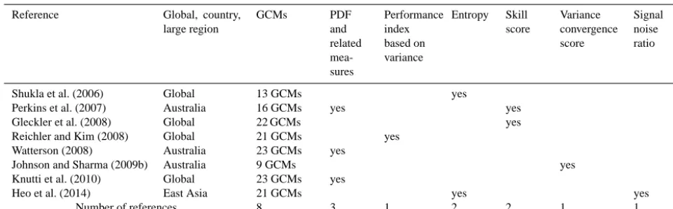
Table 2b. Ranking measures of performance assessment of CMIP3 GCMs.

Reference Global, country,

large region

GCMs PDF

and related mea-sures

Performance index based on variance

Entropy Skill

score

Variance convergence score

Signal noise ratio

Shukla et al. (2006) Global 13 GCMs yes

Perkins et al. (2007) Australia 16 GCMs yes yes

Gleckler et al. (2008) Global 22 GCMs yes

Reichler and Kim (2008) Global 21 GCMs yes

Watterson (2008) Australia 23 GCMs yes

Johnson and Sharma (2009b) Australia 9 GCMs yes

Knutti et al. (2010) Global 23 GCMs yes

Heo et al. (2014) East Asia 21 GCMs yes yes

Number of references 8 3 1 2 2 1 1

Räisänen (2007) results illustrate the wide range of model performances that exist: for precipitation, RMSE=1.35 mm day−1_{with a range of 0.97–1.86 and for} temperature, RMSE=2.32◦_{C with a range of 1.58–4.56.}

Reichler and Kim (2008) considered 14 variables covering mainly the period 1979–1999 to assess the performance of CMIP3 models using their model performance index. They concluded that there was a continuous improvement in model performance from the CMIP1 models compared to those available in CMIP3 but there are still large differences in the CMIP3 models’ ability to match observed climates. Gleck-ler et al. (2008) normalised the data in Taylor diagrams for a range of climate variables and concluded that some mod-els performed substantially better than others. However, they also concluded that it is not yet possible to answer the ques-tion: what is the best model?

Reifen and Toumi (2009) (Table 2b) using temperature anomalies observed that “. . . there is no evidence that any subset of models delivers significant improvement in predic-tion accuracy compared to the total ensemble”. On the other hand, Macadam et al. (2010) (Table 2a) assessed the per-formance of 17 CMIP3 GCMs comparing the observed and modelled temperatures over five 20-year periods and con-cluded that GCM rankings based on anomalies can be in-consistent over time, whereas rankings based on actual tem-peratures can be consistent over time.

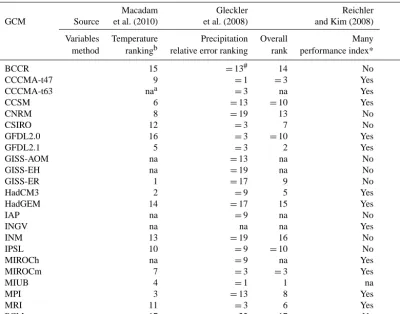
In summary, Gleckler et al. (2008) stated that the best GCM will depend on the intended application. In the over-arching project of which this study is a component, we are interested in the uncertainty in annual streamflow estimated through hydrologic simulation using GCM precipitation and temperature and how that uncertainty will affect estimates of future yield from surface water reservoir systems. Con-sequently, we are interested in which GCMs reproduce pre-cipitation and temperature satisfactory. Based on the refer-ences of Reichler and Kim (2008), Gleckler et al. (2008) and Macadam et al. (2010), the performance of 23 CMIP3 GCMs assessed at a global scale are ranked in Table 3. In

Ta-ble 3 eight models that meet the Reichler and Kim (2008) criterion are also ranked in the upper 50 % based on the Macadam et al. (2010) and Gleckler et al. (2008) references. These models are CCCMA-t47 (Canadian Centre for Climate Modeling and Analysis), CCSM (Community Climate Sys-tem Model), GFDL2.0 (Geophysical Fluid Dynamics Lab-oratory), GFDL2.1, HadCM3 (Hadley Centre for Climate Prediction and Research), MIROCm (Model for Interdisci-plinary Research on Climate), MPI (Max Planck Institute for Meteorology) and MRI (Japan Meteorological Research In-stitute).

3 Data

Two data sets are used in the GCM assessment that follows in Sect. 4. One is based on observed data and the other on GCM simulations of present climate (20C3M). It should be noted that of the 22 GCMs examined herein, multiple runs or projections were available for nine models. The resulting 46 runs are identified in the tables summarising the results.

The first data set is based on monthly observed precipita-tion and temperature gridded at 0.5◦×0.5◦ resolution over the global land surface from Climatic Research Unit (CRU) 3.10 (New et al., 2002) for the period January 1950 to De-cember 1999. For grid cells where monthly observations are not available, the CRU 3.10 data set is based on interpola-tion of observed values within a correlainterpola-tion decay distance of 450 km for precipitation and 1200 km for temperature. The CRU 3.10 data set provides information about the number of observations within the correlation decay distance of each grid cell for each month. In this analysis we defined a grid cell as observed if≥90 % of months at that grid cell has at least one observation within the correlation decay distance for the period January 1950 to December 1999. Only ob-served grid cells are used to compute summary statistics in the following analysis.

Table 3. Summary of performance of 23 CMIP3 GCMs in simulating present climate based on literature review.

Macadam Gleckler Reichler

GCM Source et al. (2010) et al. (2008) and Kim (2008)

Variables Temperature Precipitation Overall Many

method rankingb relative error ranking rank performance index*

BCCR 15 =13# 14 No

CCCMA-t47 9 =1 =3 Yes

CCCMA-t63 naa =3 na Yes

CCSM 6 =13 =10 Yes

CNRM 8 =19 13 No

CSIRO 12 =3 7 No

GFDL2.0 16 =3 =10 Yes

GFDL2.1 5 =3 2 Yes

GISS-AOM na =13 na No

GISS-EH na =19 na No

GISS-ER 1 =17 9 No

HadCM3 2 =9 5 Yes

HadGEM 14 =17 15 Yes

IAP na =9 na No

INGV na na na Yes

INM 13 =19 16 No

IPSL 10 =9 =10 No

MIROCh na =9 na Yes

MIROCm 7 =3 =3 Yes

MIUB 4 =1 1 na

MPI 3 =13 8 Yes

MRI 11 =3 6 Yes

PCM 17 22 17 No

* As summarised in Smith and Chandler (2010) (The performance index is based on the error variance between modelled and observed climate for 14 climate and ocean variables. “Yes” indicates the variance error is less than the median across the GCMs.)a_{na: not available or not}

applicable.b_{Rank 1 is best rank.}#_{more than one GCM with this rank.}

23 GCMs listed in Table 1 and consists of 46 GCM runs. The 20C3M monthly data for precipitation and temperature were extracted from the CMIP3 data set. As shown in Ta-ble 1 the GCMs have a wide range of spatial resolutions, all of which are coarser than the observed CRU data. In or-der to make comparisons between observed and GCM data either the CRU and/or GCM data must be re-sampled to the same resolution. To avoid re-sampling coarse resolution data to a finer resolution we only re-sampled the CRU data here. Thus, in the following analysis the performance of each GCM is assessed at the resolution of the GCM and the CRU data are re-sampled to match the GCM resolution. There-fore, the number of grid cells in each comparison varies with the GCM resolution and ranged from 616 to 11 886 for the temperature comparisons and 425 to 8291 for the precipi-tation comparisons. The difference in number of grid cells between temperature and precipitation is due to more terres-trial grid cells having observed temperature data than precip-itation data over the period 1950–1999.

In the following analysis comparisons are made between observed and GCM values of mean and standard deviation of annual precipitation and mean annual temperature. The

GCM values are based on concurrent raw (that is, not down-scaled nor bias corrected) data from the 20C3M simulation. For example, if a grid cell has observed calendar-year data from 1953 to 1994, then the comparison will be made with GCM values from the 20C3M run for the concurrent calendar years 1953–1994. Although the aim of a 20C3M run from a given GCM is not to strictly replicate the observed monthly record, we expect better performing GCMs to reproduce mean annual statistics that are broadly similar to observed conditions. Average monthly precipitation and temperature patterns are also compared to assess how well GCM runs re-produce observed seasonality. Finally, we assess how well the Köppen–Geiger climate classification (Peel et al., 2007) estimated from the CMIP3 data compares with present-day gridded observed climate classification.

4 Comparison of present climate GCM data with

observed data

for terrestrial grid cells with≥90 % observed data during the period 1950–1999.

Eight standard statistics – Nash–Sutcliffe efficiency (NSE) (Nash and Sutcliffe, 1970), product moment coefficient of determination (R2) (MacLean, 2005), standard error of regression (Maidment, 1992), bias (MacLean, 2005), percentage bias (Maidment, 1992), absolute percentage bias (MacLean, 2005), root mean square error (RMSE) (MacLean, 2005) and mean absolute error (MacLean, 2005) – were computed as the basis of comparison, but we report only the NSE,R2and RMSE in the following discussion. For our analysis, the NSE is the most useful statistic as it shows the proportion of explained variance relative to the 1 : 1 line in a comparison of two estimates of the same variable.R2is included because many analysts are familiar with its interpre-tation. Both NSE andR2were computed in arithmetic (un-transformed) and natural log space. We have also included RMSE values (computed from the untransformed values) as many GCM analyses include this measure.

In the following sub-sections comparisons between the concurrent raw GCM data and observed values for MAP, SDP, MAT, long-term average monthly precipitation and temperature patterns and Köppen–Geiger climate classifica-tion at the grid cell scale are presented and discussed. Al-though we rank the models by each selection criteria and combine the ranks by addition, we note the warning of Stain-forth et al. (2007) who argue that model response should not be weighted but ruled in or out. We follow this approach in this paper by identifying better performing GCMs to be used for hydrologic simulations reported in a companion paper (Peel et al., 2015). This approach is consistent with the concept recognised by Randall et al. (2007, p. 608) that “. . . for models to predict future climatic conditions reliably, they must simulate the current climatic state with some as yet unknown degree of fidelity. Poor model skill in simu-lating present climate could indicate that certain physical or dynamical processes have been misrepresented”. It is noted that our comparisons are conducted over the global terrestrial land surface rather than focussing on a single catchment, re-gion or continent. This allows us to assess whether a GCM performs consistently well across a large area and reduces the chance of a GCM being selected due to a random high performance over a small area.

4.1 Mean annual precipitation

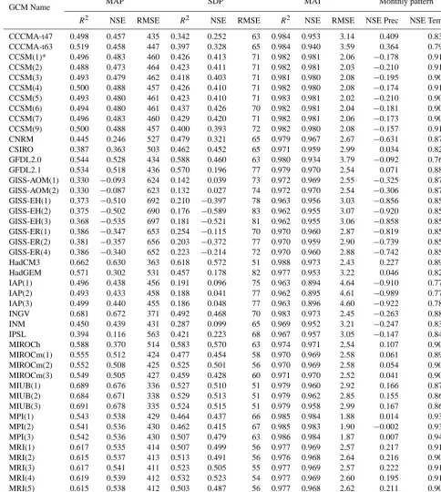
Comparisons of mean annual precipitation and the standard deviation of annual precipitation between GCM estimates and observed data for the grid cells across the 46 runs are pre-sented in Table 4. For MAP, the NSE varied from a maximum of 0.68 (R2=0.69) with a RMSE value of 335 mm year−1 for model MIUB(3) (Meteorological Institute of the Univer-sity of Bonn) to −0.54 for GISS-EH(3) (NASA Goddard Institute of Space Studies). (GCM run number is enclosed by parenthesis, for example MIUB(3) is run 3 for the GCM

y = 8.52x0.69

R² = 0.66 n = 632

10 100 1000 10000

10 100 1000 10000

GC

M

m

ea

n

annua

l g

idde

d

pr

ec

ipi

ta

tio

n

(m

m

y

ea

r

-1

)

CRU mean annual gridded precipitation (mm year-1₎ MIUB(3)

Figure 1. Comparison of MIUB(3) model estimates of observed

mean annual precipitation with CRU estimates. (Based on

untrans-formed precipitation NSE=0.678, rank 1 of 46 runs, andR2=

0.691.)

y = 2.71x0.83

R² = 0.36 n = 425

10 100 1000 10000

10 100 1000 10000

GC

M

m

ea

n

annua

l g

idde

d

pr

ec

ipi

ta

tio

n

(m

m

y

ea

r

-1

)

CRU mean annual gridded precipitation (mm year-1₎ GISS-EH(3)

Figure 2. Comparison of GISS-EH(3) model estimates of observed

mean annual precipitation with CRU estimates. (Based on

untrans-formed precipitation NSE = −0.535, rank 46 of 46 runs, and

R2=0.368.)

MIUB.) The MAP values for MIUB(3) are compared with the observed CRU MAP values in Fig. 1. Each data point in this figure represents a MAP comparison at one of the 632 MIUB(3) terrestrial grid cells where observed CRU 3.10 data were available for the period January 1950 to Decem-ber 1999. The relationship between GCM and observed MAP shown in this figure is representative of the other GCMs where high MAP is underestimated and low MAP is over-estimated. GISS-EH(3), shown in Fig. 2, is an example of a poorly performing GCM in terms of mean annual precipita-tion. Here, based on untransformed data, the NSE is−0.54 (R2=0.37) with a RMSE value of 697 mm year−1.

Table 4. Performance statistics comparing CMIP3 GCM mean and standard deviation of annual precipitation, mean annual temperature, and

mean monthly patterns of precipitation and temperature with concurrent observed data. (Analysis based on untransformed data.)

GCM Name MAP SDP MAT Monthly pattern

R2 NSE RMSE R2 NSE RMSE R2 NSE RMSE NSE Prec NSE Temp

CCCMA-t47 0.498 0.457 435 0.342 0.252 63 0.984 0.953 3.14 0.409 0.838

CCCMA-t63 0.519 0.458 447 0.397 0.328 65 0.984 0.940 3.59 0.364 0.797

CCSM(1)* 0.496 0.483 460 0.426 0.413 71 0.982 0.981 2.06 −0.178 0.910

CCSM(2) 0.488 0.473 464 0.423 0.411 71 0.982 0.981 2.03 −0.210 0.912

CCSM(3) 0.493 0.479 462 0.418 0.403 71 0.981 0.980 2.08 −0.195 0.908

CCSM(4) 0.500 0.488 457 0.426 0.410 71 0.982 0.980 2.08 −0.174 0.911

CCSM(5) 0.493 0.480 461 0.423 0.410 71 0.983 0.981 2.02 −0.210 0.909

CCSM(6) 0.494 0.480 461 0.437 0.426 70 0.982 0.981 2.04 −0.181 0.909

CCSM(7) 0.496 0.483 460 0.429 0.420 71 0.982 0.981 2.06 −0.173 0.907

CCSM(9) 0.500 0.488 457 0.400 0.393 72 0.982 0.980 2.08 −0.157 0.910

CNRM 0.445 0.246 527 0.479 0.321 65 0.979 0.967 2.67 −0.631 0.879

CSIRO 0.387 0.363 503 0.462 0.452 65 0.971 0.959 2.99 0.034 0.825

GFDL2.0 0.544 0.528 434 0.588 0.460 63 0.980 0.934 3.79 −0.092 0.760

GFDL2.1 0.534 0.518 436 0.570 0.196 77 0.979 0.970 2.54 0.071 0.884

GISS-AOM(1) 0.330 −0.093 624 0.142 0.039 73 0.972 0.969 2.55 −0.325 0.873

GISS-AOM(2) 0.330 −0.087 623 0.132 0.027 74 0.972 0.970 2.54 −0.306 0.876

GISS-EH(1) 0.373 −0.510 692 0.210 −0.397 78 0.963 0.956 3.03 −0.856 0.858

GISS-EH(2) 0.375 −0.502 690 0.176 −0.589 83 0.962 0.955 3.07 −0.920 0.852

GISS-EH(3) 0.368 −0.535 697 0.181 −0.521 81 0.962 0.955 3.06 −0.858 0.856

GISS-ER(1) 0.386 −0.347 653 0.254 −0.115 70 0.970 0.960 2.87 −0.819 0.854

GISS-ER(2) 0.381 −0.357 656 0.203 −0.372 77 0.970 0.959 2.90 −0.739 0.850

GISS-ER(4) 0.386 −0.340 652 0.223 −0.214 72 0.970 0.960 2.88 −0.742 0.854

HadCM3 0.662 0.630 363 0.618 0.572 51 0.988 0.973 2.43 0.227 0.893

HadGEM 0.571 0.302 531 0.457 0.178 82 0.977 0.953 3.22 0.046 0.824

IAP(1) 0.496 0.438 456 0.191 0.096 75 0.963 0.894 4.64 −0.910 0.777

IAP(2) 0.493 0.433 458 0.188 0.041 77 0.962 0.895 4.61 −0.989 0.779

IAP(3) 0.499 0.440 455 0.186 0.048 77 0.963 0.896 4.60 −0.922 0.781

INGV 0.681 0.672 371 0.492 0.468 70 0.983 0.973 2.45 −0.263 0.882

INM 0.450 0.439 431 0.287 0.099 65 0.969 0.952 3.21 −0.247 0.833

IPSL 0.394 0.116 563 0.421 0.223 68 0.967 0.957 3.05 −0.147 0.846

MIROCh 0.588 0.370 514 0.583 0.570 63 0.974 0.971 2.54 0.107 0.906

MIROCm(1) 0.555 0.512 424 0.477 0.454 58 0.970 0.969 2.58 0.061 0.899

MIROCm(2) 0.552 0.508 425 0.525 0.501 56 0.970 0.969 2.58 0.054 0.900

MIROCm(3) 0.549 0.505 427 0.459 0.428 60 0.971 0.970 2.52 0.041 0.902

MIUB(1) 0.689 0.676 336 0.527 0.510 51 0.979 0.960 2.92 0.166 0.870

MIUB(2) 0.684 0.671 338 0.529 0.513 51 0.979 0.962 2.85 0.155 0.867

MIUB(3) 0.691 0.678 335 0.524 0.515 51 0.979 0.958 2.99 0.167 0.860

MPI(1) 0.543 0.538 429 0.464 0.437 66 0.985 0.984 1.88 0.014 0.939

MPI(2) 0.541 0.536 430 0.462 0.415 67 0.985 0.983 1.90 −0.002 0.939

MPI(3) 0.542 0.536 430 0.507 0.479 63 0.986 0.984 1.87 0.007 0.940

MRI(1) 0.617 0.535 414 0.507 0.499 56 0.977 0.969 2.57 0.217 0.912

MRI(2) 0.615 0.537 413 0.513 0.491 56 0.976 0.968 2.64 0.216 0.907

MRI(3) 0.617 0.541 411 0.523 0.505 55 0.977 0.969 2.57 0.222 0.911

MRI(4) 0.619 0.539 412 0.532 0.523 54 0.977 0.969 2.60 0.195 0.911

MRI(5) 0.615 0.538 412 0.503 0.487 56 0.977 0.968 2.62 0.211 0.907

PCM 0.360 0.190 546 0.336 0.135 73 0.975 0.943 3.49 −0.415 0.798

CCM A t4 7 CCM A t6 3 CCS M CN RM CS IR O GFDL 2. 0 GFDL 2. 1 GI SS A O M GI SS E

H _GISS E

R Had CM 3 Had GE M IA P IN GV IN M IPS

L M

IR

O

CH _MIRO

CM M IUB M PI MR I PC M -0.8 -0.6 -0.4 -0.2 0 0.2 0.4 0.6 0.8 NSE m od el led v er su s g rid ded MA P es tim at es

Figure 3. Nash–Sutcliffe efficiency (NSE) values for modelled

ver-sus observed MAP untransformed estimates for 46 CMIP3 GCM runs.

y = 8.40x0.54

R² = 0.58 n = 632

10 100 1000

10 100 1000

GC M st anda rd de vi at io n o f a nnua l g ridde d pr ec ip ita tio n ( m m y ea r -1)

CRU standard deviation of annual gridded precipitation (mm year-1₎

MIUB(3)

Figure 4. Comparison of MIUB(3) model estimates of the standard

deviation of annual precipitation with CRU observed estimates.

(Based on untransformed precipitation NSE=0.515, rank 4 of 46

runs, andR2=0.524.)

the average observed MAP across all grid cells (Gupta et al., 2009).

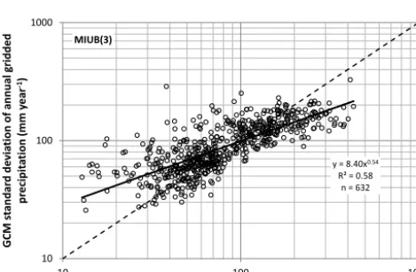
4.2 Standard deviation of annual precipitation

For the standard deviation of annual precipitation, HadCM3 was the best performing model with a NSE of 0.57, R2of 0.62 and a RMSE of 51 mm year−1_{. MIROCh also yielded} a NSE of 0.57 and an R2 of 0.58 but with a RMSE of 63 mm year−1_{. These results along with other standard} de-viation values are listed in Table 4. Figure 4 is a plot for MIUB(3), which is representative (rank 4, that is the fourth best performance of the 46 runs) of the relationship between GCM and observed SDP, and shows the model underesti-mates the standard deviation of annual precipitation for high values and overestimates at low values of standard deviation compared with observed values.

y = 1.063x - 2.25 R² = 0.98

n = 632

-40 -30 -20 -10 0 10 20 30 40

-40 -30 -20 -10 0 10 20 30 40

GC M m ea n annua l g ridde d te m pe ra tur e ( oC)

CRU mean annual gridded temperature(o_C) MIUB(3)

Figure 5. Comparison of MIUB(3) model estimates of mean annual

temperature with CRU estimates. (Based on untransformed

temper-ature NSE=0.958, rank 33 of 46 runs, andR2=0.979.)

4.3 Mean annual temperature

The comparison of the GCM mean annual temperatures with concurrent observed data for the grid cells are listed for each model run in Table 4. In contrast to the precipitation mod-elling, the mean annual temperatures are simulated satis-factorily by most of the GCMs. Except for the IAP (Insti-tute of Atmospheric Physics, Chinese Acad. Sciences) and the GFDL2.0 models (NSE= ∼0.90 and 0.93, respectively), all model runs exhibit NSE values ≥0.94 with 17 of the 46 GCM runs having a NSE value≥ 0.97. A comparison between MIUB(3) estimates of mean annual temperature (NSE=0.96, rank 33) and observed values from the CRU data set is presented in Fig. 5. Also shown in Fig. 5 is a lin-ear fit between GCM and observed MAT. The average fit for the 46 GCM runs (not shown) exhibited a small negative bias of−1.03◦_{C and a slope of 1.01.}

4.4 Average monthly precipitation and temperature

patterns

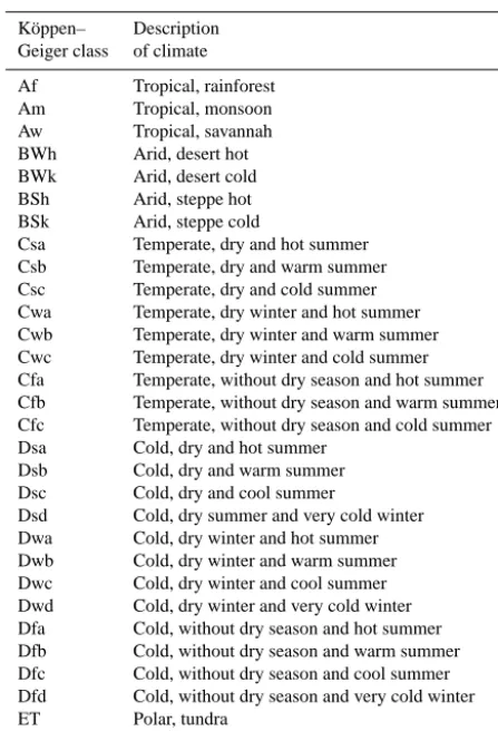
Table 5. Köppen–Geiger climate classification (adapted from Peel

et al., 2007).

Köppen– Description

Geiger class of climate

Af Tropical, rainforest

Am Tropical, monsoon

Aw Tropical, savannah

BWh Arid, desert hot

BWk Arid, desert cold

BSh Arid, steppe hot

BSk Arid, steppe cold

Csa Temperate, dry and hot summer

Csb Temperate, dry and warm summer

Csc Temperate, dry and cold summer

Cwa Temperate, dry winter and hot summer

Cwb Temperate, dry winter and warm summer

Cwc Temperate, dry winter and cold summer

Cfa Temperate, without dry season and hot summer

Cfb Temperate, without dry season and warm summer

Cfc Temperate, without dry season and cold summer

Dsa Cold, dry and hot summer

Dsb Cold, dry and warm summer

Dsc Cold, dry and cool summer

Dsd Cold, dry summer and very cold winter

Dwa Cold, dry winter and hot summer

Dwb Cold, dry winter and warm summer

Dwc Cold, dry winter and cool summer

Dwd Cold, dry winter and very cold winter

Dfa Cold, without dry season and hot summer

Dfb Cold, without dry season and warm summer

Dfc Cold, without dry season and cool summer

Dfd Cold, without dry season and very cold winter

ET Polar, tundra

EF Polar, frost

NSE value of<0. For these GCMs their predictive power for the monthly precipitation pattern is less than using the aver-age of the 12 monthly values at each of the terrestrial grid cells. Only two GCMs have NSE values>0.25. In contrast, the median NSEs of all monthly temperature patterns are

>0.75, with 41 %>0.90. The NSE metric reflects how well the GCM replicates both the monthly pattern and the over-all average monthly value (bias). Thus, the monthly pattern of temperature is generally well reproduced by the GCMs, whereas the monthly pattern of precipitation is not, which is mainly due to the bias in the GCM average monthly precipi-tation.

4.5 Köppen–Geiger classification

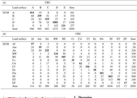
The Köppen–Geiger climate classification (Peel et al., 2007) (see Table 5) provides an alternate way to assess the ad-equacy of how well a GCM represents climate because the classification is based on a combination of annual and monthly precipitation and temperature data. Two compar-isons between the MPI(3) model and CRU observed data are presented in Table 6. The MPI(3) was chosen as an example here as over the three levels of climate classes it estimated the

observed climate correctly more often than the other model runs. In Table 6a a comparison at the first letter level of the Köppen–Geiger climate classification is shown. This com-parison reveals how well the GCM reproduces the distribu-tion of broad climate types: tropical, arid, temperate, cold and polar over the terrestrial surface. In Table 6b the comparison shown is for the second letter level of the Köppen–Geiger climate classification, which assesses how well the GCM re-produces finer detail within the broad climate types; for ex-ample, the seasonal distribution of precipitation or whether a region is semi-arid or arid. The bold diagonal values shown in Table 6a and b represent the number of grid cells correctly classified by the GCM, whereas the off-diagonal values are the number of grid cells incorrectly classified by the GCM for the one- and two-letter level. At the first letter level MPI(3) reproduces the correct climate type at 81 % of the terrestrial grid cells. Within this good performance the MPI(3) pro-duces more polar climate and fewer tropical and cold grids cells than observed. At the second letter level, MPI(3) repro-duces the correct climate type at 67 % of the terrestrial grid cells. The model produces fewer grid cells of tropical rain-forest, cold with a dry winter and cold without a dry season than expected and more cold with a dry summer and polar tundra than expected.

Table 6. Köppen–Geiger climate estimated by MPI(3) compared with the observed Köppen–Geiger climate for (a) the one-letter and (b) the

two-letter climate classification. Bold values are correctly classified grid cells.

(a) CRU

Land surface A B C D E Sum

GCM A 414 19 8 0 0 441

B 68 339 52 17 0 476

C 24 62 319 27 0 432

D 0 76 16 1085 17 1194

E 0 6 7 143 121 277

Sum 506 502 402 1272 138 2820

(b) CRU

Land surface Af Am Aw BW BS Cs Cw Cf Ds Dw Df ET EF Sum

GCM Af 57 0 2 0 0 0 0 0 0 0 0 0 0 59

Am 24 19 13 0 0 0 0 0 0 0 0 0 0 56

Aw 25 49 225 0 19 0 4 4 0 0 0 0 0 326

BW 2 1 2 134 50 3 4 0 0 0 2 0 0 198

BS 4 11 48 50 105 13 19 13 4 0 11 0 0 278

Cs 0 0 0 10 18 35 9 20 1 0 6 0 0 99

Cw 0 1 17 0 5 0 62 1 0 1 0 0 0 87

Cf 2 2 2 3 26 1 35 156 0 0 19 0 0 246

Ds 0 0 0 0 33 2 1 1 38 1 40 0 0 116

Dw 0 0 0 0 5 0 1 0 0 102 2 0 0 110

Df 0 0 0 3 35 0 4 7 2 57 843 17 0 968

ET 0 0 0 0 6 2 2 3 8 22 113 93 0 249

EF 0 0 0 0 0 0 0 0 0 0 0 11 17 28

Sum 114 83 309 200 302 56 141 205 53 183 1036 121 17 2820

y = 5E-06x + 0.4519 R² = 0.0102

y = -2E-06x + 0.9648 R² = 0.0986

-0.6 -0.4 -0.2 0 0.2 0.4 0.6 0.8 1

0 2000 4000 6000 8000 10000 12000

NS

E

val

ue

s f

or

MA

P

an

d MA

T

Number of terrestrial GCM grid cells for precipitation and temperature

MAP MAT

Figure 6. Relating 22 CMIP3 GCM resolutions (as the number

of terrestrial grid cells for MAP) to model performance based on Nash–Sutcliffe efficiency (NSE) for mean annual precipitation and mean annual temperature. (The trend lines are fitted to data with

>1500 grid cells.)

5 Discussion

5.1 Relating GCM resolution to performance

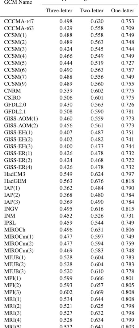
Table 7. Proportion of CMIP3 GCM grid cells (20C3M) that

repro-duce observed CRU Köppen–Geiger climate classification over the period January 1950–December 1999.

GCM Name Köppen–Geiger climate class*

Three-letter Two-letter One-letter

CCCMA-t47 0.498 0.620 0.753

CCCMA-t63 0.429 0.558 0.709

CCSM(1) 0.488 0.558 0.749

CCSM(2) 0.489 0.563 0.748

CCSM(3) 0.424 0.545 0.744

CCSM(4) 0.466 0.549 0.749

CCSM(5) 0.444 0.519 0.727

CCSM(6) 0.490 0.563 0.757

CCSM(7) 0.488 0.556 0.749

CCSM(9) 0.489 0.560 0.755

CNRM 0.539 0.602 0.775

CSIRO 0.506 0.601 0.775

GFDL2.0 0.430 0.563 0.726

GFDL2.1 0.508 0.590 0.781

GISS-AOM(1) 0.460 0.559 0.773

GISS-AOM(2) 0.456 0.561 0.773

GISS-EH(1) 0.407 0.487 0.751

GISS-EH(2) 0.402 0.482 0.741

GISS-EH(3) 0.400 0.473 0.744

GISS-ER(1) 0.426 0.478 0.732

GISS-ER(2) 0.424 0.468 0.722

GISS-ER(4) 0.426 0.478 0.732

HadCM3 0.549 0.624 0.797

HadGEM 0.563 0.676 0.818

IAP(1) 0.362 0.484 0.790

IAP(2) 0.368 0.480 0.784

IAP(3) 0.369 0.490 0.784

INGV 0.495 0.616 0.815

INM 0.452 0.526 0.731

IPSL 0.459 0.544 0.749

MIROCh 0.496 0.631 0.806

MIROCm(1) 0.477 0.597 0.749

MIROCm(2) 0.477 0.594 0.759

MIROCm(3) 0.469 0.583 0.748

MIUB(1) 0.528 0.604 0.783

MIUB(2) 0.528 0.604 0.783

MIUB(3) 0.520 0.610 0.778

MPI(1) 0.599 0.666 0.801

MPI(2) 0.593 0.657 0.805

MPI(3) 0.602 0.669 0.808

MRI(1) 0.534 0.644 0.808

MRI(2) 0.521 0.625 0.798

MRI(3) 0.527 0.632 0.798

MRI(4) 0.528 0.634 0.799

MRI(5) 0.532 0.641 0.803

PCM 0.397 0.481 0.660

* The three-, two- and one-letter climate classes are listed in Table 5.

Table 8. CMIP3 GCM run rank (rank 1=best) based on Nash– Sutcliffe efficiency (NSE) values from comparison of 20C3M and concurrent observed grid cell data.

GCM MAP SDP MAT Monthly Rank Overall

Name rank rank rank pattern rank* sum GCM rank

CCCMA-t47 28 30 38 19 115 12

CCCMA-t63 27 28 42 22 119 13

CCSM(1) 21 22 7 18 68 8

CCSM(2) 26 23 5 17 71

CCSM(3) 25 26 10 21 82

CCSM(4) 20 25 11 16 72

CCSM(5) 24 24 4 21 73

CCSM(6) 23 19 6 20 68

CCSM(7) 22 20 8 19.5 69.5

CCSM(9) 19 27 9 17 72

CNRM 36 29 26 30.5 121.5 14

CSIRO 34 16 32 28.5 110.5 11

GFDL2.0 14 14 43 34 105 10

GFDL2.1 15 32 15 17.5 79.5 9

GISS-AOM(1) 40 39 20 30.5 129.5

GISS-AOM(2) 39 40 17 29.5 125.5 15

GISS-EH(1) 45 44 35 35.5 159.5 22

GISS-EH(2) 44 46 37 39 166

GISS-EH(3) 46 45 36 36.5 163.5

GISS-ER(1) 42 41 28 36 147 19

GISS-ER(2) 43 43 31 36.5 153.5

GISS-ER(4) 41 42 29 36 148

HadCM3 5 1 13 12 31 1

HadGEM 35 33 39 28 135 17

IAP(1) 31 36 46 44 157

IAP(2) 32 38 45 45 160

IAP(3) 29 37 44 44 154 21

INGV 3 13 12 28 56 5

INM 30 35 40 35 140 18

IPSL 38 31 34 29.5 132.5 16

MIROCh 33 2 14 14.5 63.5 7

MIROCm(1) 16 15 22 17 70

MIROCm(2) 17 8 21 17 63 6

MIROCm(3) 18 18 16 17.5 69.5

MIUB(1) 2 6 30 18.5 56.5

MIUB(2) 4 5 27 19.5 55.5 4

MIUB(3) 1 4 33 19 57

MPI(1) 9 17 2 10.5 38.5

MPI(2) 12 21 3 12 48

MPI(3) 11 12 1 10.5 34.5 2

MRI(1) 13 9 18 5 45

MRI(2) 10 10 25 10.5 55.5

MRI(3) 6 7 19 5.5 37.5 3

MRI(4) 7 3 23 8 41

MRI(5) 8 11 24 11.5 54.5

PCM 37 34 41 38.5 150.5 20

* Monthly pattern rank is the rank of the average of the monthly pattern NSEs for precipitation and temperature.

model development. Our observation is consistent with Mas-son and Knutti (2011) who comment that “. . . model reso-lution in CMIP3 seems to only affect performance in sim-ulating present-day temperature for small scales over land” (p. 2691) and for precipitation they comment that “. . . no clear relation seems to exist at least within the relatively nar-row range of resolutions covered by CMIP3“ (p. 2686).

5.2 Joint comparison of precipitation and temperature

Table 9. Better performing CMIP3 GCMs identified from the

liter-ature and our analyses.

Grid cells Literature Better performing

(Tables 4 and 8) (Table 3) GCMs

(Col. 1) (Col. 2) (Col. 3)

CCCMA-t47 CCSM GFDL2.0 GFDL2.1

HadCM3 HadCM3 HadCM3

INGV

MIROCh*

MIROCm MIROCm MIROCm

MIUB MIUB* MIUB

MPI MPI MPI

MRI MRI MRI

* Added to list – see Section 5.3 for explanation.

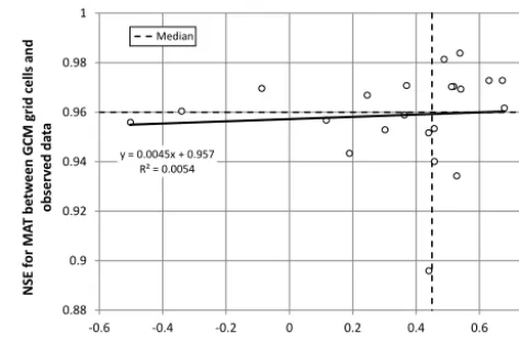
from the same GCM run. Grid cell based NSEs for mean an-nual temperature and mean anan-nual precipitation from each GCM are compared in Fig. 7, which illustrates the perfor-mance of each GCM for both variables. Models that have relatively high NSEs for precipitation do not necessarily have relatively high values for temperature. It is interesting to note that the rank of the models based on NSE of the MAP is unrelated to the ranking of the models based on MAT. For-tunately, however, most of the NSEs for MAT are relatively high and the acceptance or rejection of a GCM as a better performing model is largely dependent on its precipitation characteristics.

5.3 Identifying better performing GCMs

To identify the better performing GCMs across the differ-ent variables assessed, the results in Table 4 are ranked by NSE and summarised in Table 8. The monthly patterns of precipitation and temperature are combined by ranking the average of their respective NSE values. The overall rank for each GCM run is based on combining, by addition, the ranks for the individual variables and, finally, identifying the best performing run from each GCM. Selection of the bet-ter performing GCMs using these rankings is not inconsis-tent with Stainforth et al. (2007) who argued that model re-sponse should not be weighted but ruled in or out. From Ta-ble 8 we identify several GCMs, listed in TaTa-ble 9, as bet-ter performing models. These selected GCMs were based on the assumption that performance across the four vari-ables (MAP, SDP, MAT and combined monthly pattern) is equally weighted. GCMs that achieved MAP NSE>0.50, SDP NSE>0.45, MAT NSE>0.95 and mean monthly pat-tern of precipitation NSE>0.0 (Table 4) were identified as better performing. (Because nearly all the GCM runs mod-elled mean monthly patterns of temperature satisfactorily,

y = 0.0045x + 0.957 R² = 0.0054

0.88 0.9 0.92 0.94 0.96 0.98 1

-0.6 -0.4 -0.2 0 0.2 0.4 0.6 0.8

NSE

fo

r MA

T b

etw

een

G

CM

gr

id

c

el

ls

a

nd

ob

se

rv

ed da

ta

NSE for MAP between GCM grid cells and observed data Median

Figure 7. Comparison of Nash–Sutcliffe efficiency (NSE) values

between CMIP3 GCM and observed mean annual temperatures with NSE values between CMIP3 GCM and observed mean annual precipitation.

this measure was not considered in the selection of models listed in column 1, Table 9.) The following GCMs were se-lected (Table 9): HadCM3, INGV (National Institute of Geo-physics and Vulcanology, Italy), MIROCm, MIUB, MPI and MRI. INGV was included although it failed the monthly pre-cipitation pattern criterion. The above criteria were selected to identify a small number of GCMs that would require less bias correction to produce annual precipitation and tempera-ture consistent with observations.

1.005 1.010 1.015 1.020 1.025 1.030 1.035 1.040 1.045 1.050 1.055

0.0 0.5 1.0 1.5 2.0 2.5

Pr

ec

ip

ita

tio

n Ra

tio

∆ Temperature (o_C)

GCM runs not selected Five GCMs runs adopted median

Figure 8. Ratio of 2015–2034 to 1965–1994 mean annual

precipita-tion compared with the change in mean annual temperature (2015– 2034 to 1965–1994) for the selected five CMIP3 GCMs runs com-pared with the 23 CMIP3 GCMs including all ensemble members for the global land surface.

5.4 Comparing future responses of selected GCMs

In order to confirm that the selected GCM runs are represen-tative of the range of future responses to climate change in the CMIP3 ensemble, we plot in Fig. 8 the ratio of mean an-nual precipitation for the period 2015–2034 (from the A1B scenario) to 1965–1994 against the mean annual temperature difference between 2015–2034 and 1965–1994 for the global land surface. The five selected GCM runs are well distributed amongst the 44 GCM ensemble members, which indicates that the selected GCMs are reasonably representative of the range of future GCM projections if all the runs were consid-ered. We observe that most GCM runs are clustered around the median response, except for the seven CCSM runs in the top right quadrant with a precipitation ratio>∼1.04.

6 Conclusions

Our primary objective in this paper is to identify better per-forming GCMs from a hydrologic perspective over global land regions. The better performing GCMs were identified by their ability to reproduce observed climatological statis-tics (mean and the standard deviation of annual precipitation and mean annual temperature, and the mean monthly patterns of precipitation and temperature) for hydrologic simulation. The GCM selection process was informed by our results pre-sented here and by a literature review of CMIP3 GCM perfor-mance. In terms of the NSE there was a large spread in val-ues for mean annual precipitation and the standard deviation of annual precipitation over concurrent periods. The highest NSE for mean annual precipitation was 0.68 and 0.57 for the standard deviation of annual precipitation. On the other hand, for mean annual temperatures, the NSEs between modelled and observed data were very high, with median NSE being

0.97. Overall, all GCMs reproduced the Köppen–Geiger cli-mate satisfactorily at the broad first letter level. From the lit-erature, the following GCMs were identified as being suit-able to simulate annual precipitation and temperature statis-tics: CCCMA-T47, CCSM, GFDL2.0, GFDL2.1, HadCM3, MIROCh, MIROCm, MIUB, MPI and MRI. After combin-ing our results with the literature the followcombin-ing GCMs were considered the better performing models from a hydrologic perspective: HadCM3, MIROCm, MIUB, MPI and MRI. The future response of the better performing GCMs was found to be representative of the 44 GCM ensemble members which confirms that the selected GCMs are reasonably representa-tive of the range of future GCM projections. Our approach for evaluating GCM performance for hydrologic simulation could be applied to CMIP5 runs.

The Supplement related to this article is available online at doi:10.5194/hess-12-361-2015-supplement.

Acknowledgements. This research was financially supported

by Australian Research Council grant LP100100756 and

FT120100130, Melbourne Water and the Australian Bureau of Meteorology. Lionel Siriwardena, Sugata Narsey and Dr Ian Smith assisted with extraction and analysis of CMIP3 GCM data. Lionel Siriwardena also assisted with extraction and analysis of the CRU 3.10 data. We acknowledge the modelling groups, the Program for Climate Model Diagnosis and Intercomparison (PCMDI) and the WCRP’s Working Group on Coupled Modelling (WGCM) for their roles in making available the WCRP CMIP3 multi-model data set. Support of this data set is provided by the Office of Science, U.S. Department of Energy. The authors thank two anonymous reviewers who provided stimulating comments on the discussion paper.

Edited by: A. Loew

References

Boer, G. J. and Lambert, S. J.: Second order space–time climate difference statistics, Clim. Dynam., 17, 213–218, 2001. Bonsal, B. T. and Prowse, T. D.: Regional assessment of

GCM-simulated current climate over Northern Canada, Arctic, 59, 115–128, 2006.

Charles, S. P., Bari, M. A., Kitsios, A., and Bates, B. C.: Effect of GCM bias on downscaled precipitation and runoff projections for the Serpentine catchment, Western Australia, Int. J. Climatol., 27, 1673–1690, 2007.

Chervin, R. M.: On the Comparison of Observed and GCM Simu-lated Climate Ensembles, J. Atmos. Sci., 38, 885–901, 1981. Chiew, F. H. S. and McMahon, T. A.: Modelling the impacts of

Covey, C., Achutarao, K. M., Cubasch, U., Jones, P., Lambert S. J., Mann, M. E., Phillips, T. J., and Taylor, K. E.: An overview of results from the Coupled Model Intercomparison Project, Global Planet. Change, 37, 103–133, 2003.

Dessai, S., Lu, X., and Hulme, M.: Limited sensitivity analysis of regional climate change probabilities for the 21st century, J. Geo-phys. Res., 110, D19108, doi:10.1029/2005JD005919, 2005. Flato, G., Marotzke, J., Abiodun, B., Braconnot, P., Chou, S. C.,

Collins, W., Cox, P., Driouech, F., Emori, S., Eyring, V., Forest, C., Gleckler, P., Guilyardi, E., Jakob, C., Kattsov, V., Reason, C., and Rummukainen, M.: Evaluation of Climate Models, in: Cli-mate Change 2013: The Physical Science Basis. Contribution of Working Group I to the Fifth Assessment Report of the Intergov-ernmental Panel on Climate Change, edited by: Stocker, T. F., Qin, D., Plattner, G.-K., Tignor, M., Allen, S. K., Boschung, J., Nauels, A., Xia, Y., Bex, V., and Midgley, P. M., Cambridge Uni-versity Press, Cambridge, United Kingdom and New York, NY, USA, 2013.

Foody, G. M.: Thematic map comparison: Evaluating the statisti-cal significance of differences in classification accuracy, Pho-togramm. Eng. Remote S., 70, 627–633, 2004.

Gleckler, P. J., Taylor, K. E., and Doutriaux, C.: Performance met-rics for climate models, J. Geophys. Res.-Atmos., 113, D06104, doi:10.1029/2007JD008972, 2008.

Gupta, H. V., Kling, H., Yilmaz, K. K., and Martinez, G. F.: Decom-position of the mean squared error and NSE performance criteria: Implications for improving hydrological modelling, J. Hydrol., 377, 80–91, 2009.

Hagemann, S., Chen, C., Haerter, J. O., Heinke, J., Gerten, D., and Piani, C.: Impact of a statistical bias correction on the projected hydrological changes obtained from three GCMs and two hydrol-ogy models, J. Hydrometeorol. 12, 556–578, 2011.

Heo, K.-Y., Ha, K.-J., Yun, K.-S., Lee, S.-S., Kim, H.-J., and Wang, B.: Methods for uncertainty assessment of climate models and model predictions over East Asia, Int. J. Climatol., 34, 377–390, doi:10.1002/joc.2014.34.issue-2, 2014.

Johns, T. C., Durman, C. F., Banks, H. T., Roberts, M. J., Mclaren, A. J., Ridley, J. K., Senior, C. A., Williams, K. D., Jones, A., Rickard, G. J., Cusack, S., Ingram, W. J., Crucifix, M., Sexton, D. M. H., Joshi, M. M., Dong, B.-W., Spencer, H., Hill, R. S. R., Gregory, J. M., Keen, A. B., Pardaens, A. K., Lowe, J. A., Bodas-Salcedo, A., Stark, S., and Searl, Y.: The new Hadley Centre cli-mate model (HadGEM1): evaluation of coupled simulations, J. Climate, 19, 1327–1353, 2006.

Johnson, F. M. and Sharma, A.: GCM simulations of a future cli-mate: How does the skill of GCM precipitation simulations com-pare to temperature simulations, 18th World IMACS/MODSIM Congress, Cairns, Australia, 2009a.

Johnson, F. and Sharma, A.: Measurement of GCM skill in pre-dicting variables relevant for hydroclimatological assessments, J. Climate, 22, 4373–4382, 2009b.

Knutti, R., Furrer, R., Tebaldi, C., Cermak, J., and Meehl, G. A.: Challenges in combining projections from multiple climate mod-els, J. Climate, 23, 2739–2758, 2010.

Knutti, R., Masson, D., and Gettelman, A.: Climate model geneal-ogy: Generation CMIP5 and how we got there, Geophys. Res. Lett., 40, 1194–1199, 2013.

Lambert, S. J. and Boer, G. J.: CMIP1 evaluation and intercompari-son of coupled climate models, Clim. Dynam., 17, 83–106, 2001.

Legates, D. R. and Willmott, C. J.: A comparison of GCM-simulated and observed mean January and July precipitation, Global Planet. Change, 5, 345–363, 1992.

Macadam, I., Pitman, A. J., Whetton, P. H., and Abramowitz, G.: Ranking climate models by performance using actual values and anomalies: Implications for climate change impact assessments, Geophys. Res. Lett., 37, L16704, doi:10.1029/2010GL043877, 2010.

MacLean, A.: Statistical evaluation of WATFLOOD (Ms), Univer-sity of Waterloo, Ontario, Canada, 2005.

Maidment, D. R.: Handbook of Hydrology, McGraw-Hill Inc., New York, 1992.

Masson, D. and Knutti, R.: Spatial-scale dependence of climate model performance in the CMIP3 ensemble, J. Climate, 24, 2680-2692, 2011.

McMahon, T. A. and Adeloye, A. J.: Water Resources Yield, Water Resources Publications, CO, USA, 220 pp., 2005.

McMahon, T. A., Peel, M. C., Pegram, G. G. S., and Smith, I. N.: A simple methodology for estimating mean and variability of an-nual runoff and reservoir yield under present and future climates, J. Hydrometeorol., 12, 135–146, 2011.

Meehl, G. A., Covey, C., Delworth, T., Latif, M., McAvaney, B., Mitchell, J. F. B., Stouffer, R. J., and Taylor, K. E.: The WCRP CMIP3 multi-model dataset: A new era in climate change re-search, B. Am. Meteorol. Soc., 88, 1383–1394, 2007.

Min, S.-K. and Hense, A.: A Bayesian approach to climate model evaluation and multi-model averaging with an appli-cation to global mean surface temperatures from IPCC AR4 coupled climate models, Geophys. Res. Lett., 33, L08708, doi:10.1029/2006GL025779, 2006.

Murphy, J. M., Sexton, D. M. H., Barnett, D. N., Jones, G. S., Webb, M. J., Collins, M. J., and Stainforth, D. A.: Quantification of modelling uncertainties in a large ensemble of climate change simulations, Nature, 430, 768–772, 2004.

Nash, J. E. and Sutcliffe, J. V.: River flow forecasting through con-ceptual models Part 1 – A discussion of principles, J. Hydrol., 10, 282–290, 1970.

New, M., Lister, D., Hulme, M., and Makin, I.: A high-resolution data set of surface climate over global land areas, Clim. Res., 21, 1–25, 2002.

Peel, M. C., Finlayson, B. L., and McMahon, T. A.: Updated world map of the Köppen–Geiger climate classification, Hydrol. Earth Syst. Sci., 11, 1633-1644, doi:10.5194/hess-11-1633-2007, 2007.

Peel, M. C., Srikanthan, R., McMahon, T. A., and Karoly, D. J.: Ap-proximating uncertainty of annual runoff and reservoir yield us-ing stochastic replicates of Global Climate Model data, Hydrol. Earth Syst. Sci. Discuss., under review, 2015.

Perkins, S. E., Pitman, A. J., Holbrook, N. J., and McAneney, J.: Evaluation of the AR4 climate models simulated daily maximum temperature, minimum temperature and precipitation over Aus-tralia using probability density functions, J. Climate, 20, 4356– 4376, 2007.

Phillips, N. A.: The general circulation of atmosphere: a numerical experiment, Q. J. Roy. Meteorol. Soc., 82, 123–164, 1956. Räisänen, J.: How reliable are climate models?, Tellus A, 59, 2–29,

Raju, K. S. and Kumar, D. N.: Ranking of global climate models for India using multicriterion analysis, Clim. Res., 60, 103–117, 2014.

Randall, R. A. and Wood, R. A. (Coordinating lead authors): Climate models and their evaluation. Contribution of Working Group I to the Fourth Assessment Report of the Intergovernmen-tal Panel on Climate Change AR4, Chap. 8, 589–662, 2007. Reichler, T. and Kim, J.: How well do coupled models simulate

to-day’s climate?, B. Am. Meteorol. Soc., 89, 303–311, 2008. Reifen, C. and Toumi, R.: Climate projections: Past performance

no guarantee of future skill?, Geophys. Res. Lett., 36, L13704, doi:10.1029/2009GL038082, 2009.

Shukla, J., DelSole, T., Fennessy, M., Kinter, J., and Paolino, D.: Climate model fidelity and projections of climate change, Geo-phys. Res. Lett., 33, L07702, doi:10.1029/2005GL025579, 2006. Smith, I. and Chandler, E.: Refining rainfall projections for the Mur-ray Darling Basin of south-east Australia – the effect of sampling model results based on performance, Clima. Change, 102, 377– 393, 2010.

Stainforth, D. A., Allen, M. R., Tredger, E. R., and Smith, L. A.: Confidence, uncertainty and decision-support relevance in cli-mate predictions, Philos. T. R. Soc. A, 365, 2145–2161, 2007.

Suppiah, R., Hennessy, K. L., Whetton, P. H., McInnes, K., Macadam, I., Bathols, J., Ricketts, J., and Page, C. M.: Australian climate change projections derived from simulations performed for IPCC 4th Assessment Reportm Aust. Met. Mag, 56, 131–152, 2007.

Taylor, K. E.: Summarizing multiple aspects of model performance in a single diagram, J. Geophys. Res., 106, 7183–7192, 2001. van Oldenborgh, G. J., Philip, S. Y., and Collins, M: El Niño in

a changing climate: a multi-model study, Ocean Sci., 1, 81–95, doi:10.5194/os-1-81-2005, 2005.

Watterson, I. G.: Calculation of probability density functions for temperature and precipitation change under global warming, J. Geophys. Res., 113, D12106, doi:10.1029/2007JD009254, 2008. Whetton, P., McInnes, K. L., Jones, R. J., Hennessy, K. J., Suppiah, R., Page, C. M., and Durack, P. J.: Australian Climate Change Projections for Impact Assessment and Policy Application: A Review, CSIRO Marine and Atmospheric Research Paper 001, available at: www.cmar.csiro.au/e-print/open/whettonph_2005a. pdf, 2005.