https://doi.org/10.5194/hess-23-4851-2019 © Author(s) 2019. This work is distributed under the Creative Commons Attribution 4.0 License.
Spatially dependent flood probabilities to support
the design of civil infrastructure systems
Phuong Dong Le1,2, Michael Leonard1, and Seth Westra1
1School of Civil, Environmental and Mining Engineering, University of Adelaide, Adelaide, South Australia, Australia 2Faculty of Water Resources Engineering, Thuyloi University, 175 Tay Son, Dong Da, Hanoi, Vietnam
Correspondence:Phuong Dong Le ([email protected]) Received: 19 July 2018 – Discussion started: 4 September 2018
Revised: 23 September 2019 – Accepted: 25 September 2019 – Published: 27 November 2019
Abstract. Conventional flood risk methods typically focus on estimation at a single location, which can be inadequate for civil infrastructure systems such as road or railway infras-tructure. This is because rainfall extremes are spatially de-pendent; to understand overall system risk, it is necessary to assess the interconnected elements of the system jointly. For example, when designing evacuation routes it is necessary to understand the risk of one part of the system failing given that another region is flooded or exceeds the level at which evacuation becomes necessary. Similarly, failure of any sin-gle part of a road section (e.g., a flooded river crossing) may lead to the wider system’s failure (i.e., the entire road be-comes inoperable). This study demonstrates a spatially de-pendent intensity–duration–frequency (IDF) framework that can be used to estimate flood risk across multiple catchments, accounting for dependence both in space and across different critical storm durations. The framework is demonstrated via a case study of a highway upgrade comprising five river cross-ings. The results show substantial differences in conditional and unconditional design flow estimates, highlighting the im-portance of taking an integrated approach. There is also a reduction in the estimated failure probability of the overall system compared with the case where each river crossing is treated independently. The results demonstrate the poten-tial uses of spapoten-tially dependent intensity–duration–frequency methods and suggest the need for more conservative design estimates to take into account conditional risks.
1 Introduction
Methods for quantifying the flood risk of civil infrastructure systems such as road and rail networks require considerably more information compared to traditional methods that focus on flood risk at a point. For example, the design of evacua-tion routes requires the quantificaevacua-tion of the risk that one part of the system will fail at the same time that another region is flooded or exceeds the level at which evacuation becomes necessary. Similarly, a railway route may become impass-able if any of a number of bridges are submerged, such that the “failure probability” of that route becomes some aggre-gation of the failure probabilities of each individual section. Successful estimation of flood risk in these systems there-fore requires recognition both of the networked nature of the civil infrastructure system across a spatial domain, as well as the spatial and temporal structure of flood-producing mech-anisms (e.g., storms and extreme rainfall) that can lead to system failure (e.g., Leonard et al., 2014; Seneviratne et al., 2012; Zscheischler et al., 2018).
spa-tial copulas (Durocher et al., 2016). However, in many in-stances continuous streamflow data are unavailable or insuf-ficient at the locations of interest, or the catchment condi-tions have changed such that historical streamflow records are unrepresentative of likely future risk. For these situations, rainfall-based methods are often more appropriate.
There are two primary classes of rainfall-based methods to estimate flood probability. The first uses continuous rainfall data (either historical or generated) to compute continuous streamflow data using a rainfall-runoff model (Boughton and Droop, 2003; Cameron et al., 1999; He et al., 2011; Heg-nauer et al., 2014; Pathiraja et al., 2012), with flood risk then estimated based on the simulated streamflow time se-ries. This method is computationally intensive, and given the challenge of reproducing a wide variety of statistics across many scales, it can have difficulties in modeling the depen-dence of extremes. Most spatial rainfall models operate at the daily timescale (Bárdossy and Pegram, 2009; Baxevani and Lennartsson, 2015; Bennett et al., 2016b; Hegnauer et al., 2014; Kleiber et al., 2012; Rasmussen, 2013), whereas many catchments respond at sub-daily timescales. This is likely because the capacity of space–time rainfall models to simulate the statistics of sub-daily rainfall remains a chal-lenging research problem (Leonard et al., 2008), although one approach is to exploit the relative abundance of data at the daily scale then apply a downscaling model to reach sub-daily scales (Gupta and Tarboton, 2016). Continuous simu-lation is receiving ongoing attention and increasing applica-tion, yet there remain limitations when applying these mod-els in many practical contexts.
The second rainfall-based method proceeds by applying probability calculations on rainfall to construct “intensity– duration–frequency” curves, which are then translated to a runoff event of an equivalent probability either via empiri-cal models such as the rational method to estimate peak flow rate (Kuichling, 1889; Mulvaney, 1851) or via event-based rainfall-runoff models that are able to simulate the full flood hydrograph (Boyd et al., 1996; Chow et al., 1988; Laurenson and Mein, 1990). Regional frequency analysis is one type of method to estimate intensity–duration–frequency (IDF) val-ues, where the precision of at-site estimates is improved by pooling data from sites in the surrounding region (Hosking and Wallis, 1997). These methods can be combined with spa-tial interpolation methods to estimate parameters for any un-gauged location of interest (Carreau et al., 2013). To deter-mine an effective mean depth of rainfall over a catchment with the same exceedance probability as at a gauge location, the pointwise estimate of extreme rainfall is multiplied by an areal reduction factor (ARF) (Ball et al., 2016). However, such methods do not account for information on the spatial dependence of extreme rainfall – whether for a single storm duration or the more complex case of different durations across a region (Bernard, 1932; Koutsoyiannis et al., 1998). The underlying independence assumption prevents these ap-proaches from being applied to estimate conditional or joint
flood risk at multiple points in a catchment or across several catchments, as would be required for a civil infrastructure system.
Although multivariate approaches can be tailored to es-timate conditional and joint probabilities of extreme rain-fall for specific situations (e.g., Kao and Govindaraju, 2008; Wang et al., 2010; Zhang and Singh, 2007), the develop-ment of a unified methodology that integrates with exist-ing IDF-based flood estimation approaches remains elusive. This is particularly challenging given that it is not only necessary to account for the dependence of rainfall across space, but it is also necessary to account for the dependence across storm burst durations, as different parts of the sys-tem may be vulnerable to different critical-duration storm events. To this end, the theory of the max-stable process has been demonstrated to represent storm-level dependence (de Haan, 1984; Schlather, 2002) and used to calculate con-ditional probabilities for a spatial domain (Padoan et al., 2010). The max-stable process has also been used to repre-sent the co-occurrence of extreme daily rainfall in the French Mediterranean region (Blanchet and Creutin, 2017). Copulas including the extremaltcopula (Demarta and McNeil, 2005) and the Hüsler–Reiss copula (Hüsler and Reiss, 1989) have also been used to model rainfall dependence.
This study applies a max-stable approach with an empha-sis on practical flood estimation problems. To this end, any proposed approach needs to account for the following:
1. The spatial dependence of rainfall “events” both for single durations and also across multiple different du-rations. This was addressed by Le et al. (2018b), who linked a max-stable model with the duration-dependent model of Koutsoyiannis et al. (1998), to create a model that could be used to reflect dependencies between nearby catchments of different sizes.
2. The asymptotic properties of spatial dependence as the events become increasingly extreme, given the focus of many flood risk estimation methods on rare flood events. Recent evidence is emerging that rainfall has an asymp-totically independent characteristic (Le et al., 2018a; Thibaud et al., 2013), which means that the level of the rainfall’s dependence reduces with an increasing re-turn period (Wadsworth and Tawn, 2012). The require-ment of asymptotic independence indicates that inverted max-stable models are preferable over max-stable mod-els.
This study adapts the methods developed by Le et al. (2018b) to inverted max-stable models to derive spatially dependent IDF estimates and ARFs as the basis for transforming rainfall into flood flows. The approach is demonstrated on a highway system spanning 20 km with five separate river crossings.
given that a neighboring catchment is flooded?” (ii) “What is the probability that the overall system fails given that each bridge is designed to a specific exceedance probability event (e.g., the 1 % annual exceedance probability event)?” The method for resolving these questions represents a new ap-proach to estimate flood risk for engineering design, by fo-cusing attention on the risk of the entire system, rather than the risk of individual system elements in isolation.
In the remainder of the paper, Sect. 2 emphasizes the need for spatially dependent IDF estimates in flood risk design and is followed by Sect. 3, which outlines the case study and data used. Section 4 explains the implementation of the frame-work, including a method for analyzing the spatial depen-dence of extreme rainfall across different durations. Results on the behavior of floods due to the spatial and duration de-pendence of rainfall extremes are provided in Sect. 5. Con-clusions and discussion follow in Sect. 6.
2 The need for spatially dependent IDF estimates in flood risk estimation
The main limitation of conventional methods of flood risk estimation is that they isolate bursts of rainfall and break the dependence structure of extreme rainfall. Figure 1 demon-strates a traditional process of estimating at-site extreme rain-fall for two locations (gauge 1 and gauge 2) and three dura-tions (1, 3, and 5 h) (Stedinger et al., 1993). The process first involves extracting the extreme burst of rainfall for each site, as well as the duration and year from the continuous rainfall data, and then fitting a probability distribution (such as the generalized extreme-value distribution) to the extracted data. Figure 1 demonstrates that, through the process of convert-ing the continuous rainfall data to a series of discrete rainfall “bursts”, this process breaks the dependence both with re-spect to duration and space. Firstly, the duration dependence is broken by extracting each duration separately, whereas for the hypothetical storm in Fig. 1 it is clear that the annual maxima from some of the extreme bursts come from the same storm. Secondly, the spatial dependence is broken be-cause each site is analyzed independently. Again, for the hy-pothetical storm of Fig. 1 it can be seen that the 5 h storm has occurred at the same time across the two catchments, and this information is lost in the subsequent probability distribution curves. Lastly, there is cross-dependence in space and dura-tion. For example, the 1 h extreme from gauge 2 occurs at the same time as the 5 h extreme from gauge 1. This may be relevant if there are two catchments with times of concentra-tion matching 1 and 5 h, respectively, which can arise where catchments are neighboring or nested.
Having obtained the IDF estimates for individual locations in Fig. 1, the next step is commonly to convert this to spatial IDF maps by interpolating results between gauged locations. Figure 2 shows hypothetical IDF maps from individual sites, with a separate spatial contour map usually provided for each
storm burst duration. In a conventional application the re-spective maps are used to estimate the magnitude of extreme rainfall over catchments for a specified time of concentration. The IDF estimates are combined with an areal reduction fac-tor to determine the volume of rainfall over a region (since rainfall is not simultaneously extreme at all locations over the region). However, because the spatial dependence was broken in the IDF analysis, the ARFs come from a separate analysis and are an attempt to correct for the broken spa-tial relationship within a catchment (Bennett et al., 2016a). Lastly, the rainfall volume over the catchment is combined with a temporal pattern (i.e., the distribution of the rainfall hyetograph within a single “storm burst”) and input into a runoff model to simulate flood flow at a catchment’s out-let. Where catchment flows can be considered independently, this process has been acceptable for conventional design, but because this process does not account for dependence across durations and across a region, it is not possible to address problems that span multiple catchments, as with civil infras-tructure systems.
The process in Fig. 1 breaks out the dependence of the ob-served rainfall, which makes the conventional approach un-able to analyze the dependence of flooding at two or more separate locations. Instead, this paper advocates for spatially dependent IDF estimates that are developed by retaining the dependence of observed rainfall in the estimation of extremal rainfall. By applying spatially dependent IDF estimates to a rainfall-runoff model, it becomes possible to represent the dependence of flooding between separate locations.
3 Case study and data
The region chosen for the case study is in the Mid North Coast region of New South Wales, Australia. This region has been the focus of a highway upgrade project and has an an-nual average daily traffic volume on the order of 15 000 ve-hicles along the existing highway. The upgrade traverses a series of coastal foothills and floodplains for a total length of approximately 20 km. The project’s major river crossings consist of extensive floodplains with some marsh areas.
Figure 1.Illustration of process to estimate rainfall extremes for each individual location in a conventional flood risk approach;(a)is for gauge 1, and(b)is for gauge 2.
Table 1.Summary of case study catchment properties.
No. Catchment Area Time of
(km2) concentration (h)
1 Bellinger 772 37
2 Kalang River 341 33
3 Deep Creek 92 8
4 Nambucca (upper) 1020 38
5 Warrell Creek 294 27
different meteorological mechanisms (Zheng et al., 2015). However some spatial dependence is still likely to be present, given that extremal rainfall in the region is strongly associ-ated with “east coast low” systems off the eastern coastline, whereby extreme hourly rainfall bursts are often embedded in heavy multi-day rainfall events.
The black circles in Fig. 3 represent the sub-daily rain sta-tions used for this study. There were seven sub-daily stasta-tions selected, with 35 years of record in common for the whole region. The data were available at a 5 min interval and ag-gregated to longer durations. For convenience in comparing the times of concentration between the catchments, this study
assumes a time of concentration of 9 h for the Deep Creek catchment, while identical times of concentration of 36 h are assumed for the other four catchments.
4 Methodology
[image:4.612.69.267.448.550.2]Figure 2.Illustration of the map of the return level and how to use it in estimating flood flow using a conventional flood risk estimates approach.
Figure 3.Map of the case study in New South Wales, Australia. The black dots indicate the rainfall gauges (G. 1 to G. 7); the red line indicates the Pacific Highway upgrade project; and the blue lines indicate the main river network. The numbers from one to five indicate the locations of the main river crossings.
employed in Sect. 4.4 to transform extremal design rainfalls to corresponding flows.
4.1 Marginal model for rainfall
This study defines extremes as those greater than some thresholdu. For a largeu, the distribution ofY conditional on Y > umay be approximated by the generalized Pareto dis-tribution (GPD) (Pickands, 1975; Davison and Smith, 1990; Thibaud et al., 2013).
G(y)=1−
1+ξ(y−u)
σu
−1/ξ
, y > u, (1)
defined on {y:1+ξ(y−u)/σu>0}, where σu>0 and −∞< ξ <+∞ are scale and shape parameters, respec-tively. The probability that a levely is exceeded is8u{1−
G(y)}, where8u=Pr(Y > u).
[image:5.612.48.287.393.588.2]fol-Figure 4.The flow chart for the overall methodology.
low a GPD (Coles, 2001). To construct IDF maps across the region, the parameters of the GPD are interpolated across the region using a thin plate spline with covariates of longitude and latitude. Though more detailed modeling of covariates could be used to improve estimates (Le et al., 2018b), the in-terpolation used here is sufficient for demonstrating the over-all method.
4.2 Dependence model for spatial rainfall
Consider rainfall as a stationary stochastic process,Zi,
asso-ciated with a location,xi, and a specific duration (the
nota-tion is simplified fromZ(xi)toZi). An important property
of dependence in the extremes is whether or not two vari-ables are likely or unlikely to co-occur as the extremes be-come rarer, as this can significantly influence the estimated frequency of flood events of a large magnitude. This is re-ferred to as asymptotic dependence or independence, respec-tively. For the case of asymptotic independence, the depen-dence structure becomes weaker as the extremal threshold increases, which is defined asP{Z1> z|Z2> z} =0 for all x16=x2. The spatial extent of a rainfall event with asymp-totically independent extremes will diminish as its rarity increases. This study uses an asymptotically independent model, of which multiple types are valid including the Gaus-sian copula (Davison et al., 2012) and inverted max-stable processes (Wadsworth and Tawn, 2012). The inverted max-stable model was ultimately selected in this study to provide consistency with earlier research (Le et al., 2018a), in which it was demonstrated to preserve the spatial properties of ex-treme rainfall in an Australian context, including the property of asymptotic independence. Thibaud et al. (2013) also com-pared the inverted max-stable model with a Gaussian copula in a case study in Switzerland, and they identified that the inverted max-stable model was appropriate.
The dependence structure of the inverted max-stable pro-cess is represented by the pairwise residual tail dependence coefficient (Ledford and Tawn, 1996). For a generic contin-uous process,Zi, for a given duration and associated with a
specific location,xi, the empirical pairwise residual tail
de-pendence coefficientηfor each pair of locations (x1,x2) is
η (x1, x2)=
logP{Z2> z}
logP{Z1> z, Z2> z}. (2)
The value ofη∈(0, 1] indicates the level of extremal de-pendence betweenZ1andZ2(Coles et al., 1999), with lower values indicating lower dependence. An example of how to calculate the residual tail dependence coefficient is provided in Appendix A for a sample dataset. To estimate the depen-dence structure of an inverted max-stable model, the theoret-ical residual tail dependence coefficient function is fitted to its empirical counterpart. Here the residual tail dependence coefficient function is assumed to only depend on the Eu-clidean distance between two locations,h= |x1−x2k. The theoretical residual tail dependence coefficient function for the Brown–Resnick model is given as
η(h)= 1
28
q
γ (h)
2
, (3)
where8is the standard normal cumulative distribution func-tion,his the distance between two locations, andγ (h) be-longs to the class of variogramsγ (h)= |h|β/qforq >0 and β∈(0, 2). The model is fitted to the empirical residual tail dependence coefficient by modifying parametersqandβ un-til the sum of squared errors is minimized.
When the extreme rainfall at locationx1andx2are of dif-ferent durations, the dependence is less than when the ex-tremes are of the same duration. For example, at a single lo-cation (h=0), when the duration is the same, the rainfall values are identical and have perfect dependence, but when the duration of extremes are different, the values are not iden-tical, and the dependence is less. An adjustment needs to be made to the theoretical pairwise residual tail dependence co-efficient function when extreme rainfalls have different dura-tions.
Following Le et al. (2018b), an adjusted approach is used by adding a nugget to the variogram as
γad.(h)=hβ/q+c(D−d)/d, (4)
[image:6.612.124.470.65.173.2]this paper), andcis a parameter to adjust dependence accord-ing to duration. This adjustment is intended to condition the behavior of shorter duration extremes on a Dhour extreme of specified magnitude. It is constructed to reflect the fact that when compared to aDhour extreme, a shorter duration results in less extremal dependence. Cases involving condi-tioning of longer periods on shorter periods (such as a 36 h extreme given a 9 h extreme has occurred) can also use the relationship in Eq. (4), but these are with different parameter values.
To fit the inverted max-stable process for all pairs of du-rations at locationsx1andx2(i.e., 36 and 12 h, 36 and 9 h, 36 and 6 h, 36 and 2 h, and 36 and 1 h), the theoretical pair-wise residual tail dependence coefficient function in Eq. (3) is used with the adjusted variogram from Eq. (4), where the parametersβ andq are first obtained from the fitted results of the case of identical 36 h durations at locationsx1andx2. The parametercis obtained by a least-square fit of the resid-ual tail dependence coefficient across all durations.
4.3 Simulation-based estimation of areal and joint rainfall
The dependence model specification in the previous section enables the calculation of joint and conditional probabilities (Appendix B). Therefore, in addition to traditional IDF return level maps that are based on independence between locations and durations, it is possible to account for the coincidence of rainfall within the region. Current design procedures using IDF estimates are event-based and rely on ancillary steps to reconstruct elements of the design storm that were broken during the estimation procedure. One critical element is the areal reduction factor, which can also be estimated by using the dependence model. ARFs are used to adjust rainfall at a point (such as the centroid of a catchment) to an effective mean rainfall over the catchment with an equivalent probabil-ity of exceedance (Ball et al., 2016; Le et al., 2018a). ARFs can be estimated from observed rainfall data, but it is difficult to extrapolate them for long return periods from observations with just 35 years of record for this study. To deal with this difficulty and to analyze the asymptotic behavior of ARFs, Le et al. (2018a) proposed a framework to simulate ARFs using the same inverted max-stable-process model adopted here. The simulation procedure from Le et al. (2018a) is sum-marized according to two steps. In the first step, the theoreti-cal residual tail dependence coefficient function in Eq. (3) is fitted to observed rainfall for the duration of interest to ob-tain the variogram parametersq >0 andβ∈(0,2). The in-verted Brown–Resnick process is obtained from a simulation of the Brown–Resnick process using the algorithm of Dom-bry et al. (2016) over a spatial domain. In the second step, the simulation in step 1 is transformed from unit Fréchet mar-gins to the rainfall-scaled marmar-gins (inverse transformation of Eq. B1). For rainfall magnitudes above the threshold the gen-eralized Pareto distribution in Eq. (1) is used, and below the
threshold the empirical distribution is used. The empirical distributions at ungauged sites are derived from the nearest gauged sites and use the interpolated response surface of the GPD threshold parameter.
An advantage of the simulation approach is that it can reflect the proportion of dry days in the empirical distribu-tion by making the simulated rainfall contain zero values (Thibaud et al., 2013). Another advantage is that the use of empirical distributions guarantees that the marginal dis-tributions of simulated rainfall below the threshold match the observed marginal distributions. There may be a draw-back by forcing the simulated rainfall to have the same ex-tremal dependence structure for both parts below and above the threshold, which may not be true for non-extreme fall. However, the dependence structure of non-extreme rain-fall contributes insignificantly to extreme events (Thibaud et al., 2013) and is unlikely to affect the results.
For calculating ARFs, the simulation is implemented sep-arately for spatial rainfall with a 36 and 9 h duration. ARFs are calculated for each duration and different return periods, which can be found in the Supplement (Figs. S1 and S2). Fig-ures S1 and S2 provide relationships between ARFs and area (in km2) for different return periods for the case study catch-ments simulated using the inverted Brown–Resnick process over equally sized grid points. The relationships are interpo-lated to obtain the ARFs for each subcatchment.
4.4 Transforming rainfall extremes to flood flow To estimate flood flow from rainfall extremes, the Watershed Bounded Network Model (WBNM) (Boyd et al., 1996) is employed. The WBNM calculates flood runoff from rain-fall hyetographs that represent the relationship between the rainfall intensity and time (Chow et al., 1988). It divides the catchment into subcatchments, allowing hydrographs to be calculated at various points within the catchment and the spa-tial variability of rainfall and rainfall losses to be modeled. It separates overland flow routing from channel routing, allow-ing changes to either or both of these processes, for example, in urbanized catchments. The rainfall extremes are estimated at the centroid of the catchment, and they are converted to av-erage spatial rainfall using the simulated ARFs described in Sect. 4.3. Design rainfall hyetographs are used to convert the rainfall magnitude to absolute values through the duration of a storm following standard design guidance in Australia (Ball et al., 2016).
Hydrological models (WBNM) for the case study area were developed and calibrated in previous studies (WMAWa-ter, 2011). Hydrological model layouts for the Bellinger, Kalang River, Nambucca, Warrell, and Deep Creek catch-ments can be found in the Supplement (Figs. S3 to S5).
5 Results
5.1 Model evaluation for the space-duration rainfall process
A GPD with an appropriate threshold was fitted to the ob-served rainfall data for 36 and 9 h durations, and the Brown– Resnick inverted max-stable-process model was calibrated to determine the spatial dependence.
Analysis of the rainfall records led to the selection of a threshold of 0.98 for all records as was reasonable across the spatial domain, and the GPD was fitted to data above the selected threshold. Figure 5 shows Q–Q plots of the marginal estimates for a representative station for two du-rations (36 and 9 h). Overall the quality of fitted distributions is good, and plots for all other stations can be found in the Supplement (Figs. S6 and S7).
The inverted max-stable process across different durations was calibrated to determine dependence parameters. The the-oretical pairwise residual tail dependence coefficient func-tion between two locafunc-tions (x1andx2) was calculated based on Eqs. (3) and (4), and the observed pairwise residual tail dependence coefficientηwas calculated using Eq. (2). Fig-ure 6 shows the pairwise residual tail dependence coefficients for the Brown–Resnick inverted max-stable process vs. dis-tance. The black points are the observed pairwise residual tail dependence coefficients, while the red lines are the fit-ted pairwise residual tail dependence coefficient functions. A coefficient equal to 1 indicates complete spatial
depen-Figure 5.Q–Qplots for the fitted GPD at one representative station. Dotted lines are the 95 % confidence bounds, and the solid diagonal line indicates a perfect fit.
dence, and a value of 0.5 indicates complete spatial inde-pendence. Figure 6a shows the dependence between 36 h ex-tremes across space, with the distanceh=0 corresponding to “complete dependence”. It also shows the dependence de-creasing with an inde-creasing distance. Figure 6 indicates that the model has a reasonable fit to the observed data given the small number of dependence parameters. Although the theoretical coefficient (red line) does not perfectly match at long distances, the main interest for this case study is in short distances, including ath=0 for the case of dependence be-tween two different durations at the same location.
Figure 6b–d show the dependence of 36 vs. 9 h extremes, 36 vs. 6 h extremes, and 36 vs. 3 h extremes, with the lat-ter two duration combinations not being used directly in the study but nonetheless showing the model performance across several durations. As expected, the dependence levels are weaker compared with 36 vs. 36 h extremes at the same dis-tance, especially at a distance of zero. This is expected, as extremes of different durations are more likely to arise from different storm events compared to storms of the same dura-tion.
5.2 Estimating conditional rainfall return levels and corresponding conditional flows for evacuation route design
[image:8.612.311.547.65.184.2]Figure 6.Plots of the pairwise residual tail dependence coefficient (TDC) against distance for 36 h extremes and 36 h extremes(a), for 36 h extremes and 9 h extremes(b), for 36 h extremes and 6 h extremes(c), and for 36 h extremes and 3 h extremes(d). The black points are the estimated residual tail dependence coefficients for pairs of sub-daily stations, and the red lines are the theoretical residual tail dependence coefficient function.
corresponding unconditional and conditional flows are given in Fig. 9.
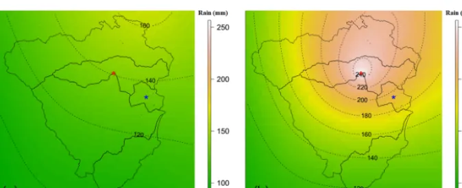
Figure 7a provides the pointwise 10-year unconditional re-turn level map over the case study area for 36 h rainfall ex-tremes. The value at the location of interest – the blue star (the centroid of the Bellinger catchment) – is around 260 mm. Figure 7b indicates that when accounting for the effect of a 20-year event for 36 h rainfall extremes happening at the lo-cation of the red star (the centroid of the Kalang River catch-ment), the pointwise 1-in-10 chance conditional return level at the blue star rises to around 453 mm (i.e., 1.74 times the unconditional value).
Figure 8 provides similar plots to Fig. 7 for another pair of locations having different durations of rainfall extremes due to different times of concentration in each catchment. Here, the location of interest is the centroid of the Deep Creek catchment (the blue star in Fig. 8), and the condi-tional point is the centroid of the Kalang River catchment (the red star in Fig. 8). The pointwise 10-year unconditional and 1-in-10 chance conditional return levels at the location of the blue star are 134 and 194 mm, respectively. The relative difference between the conditional and unconditional return levels is only 1.45 times, compared with 1.74 times for the case in Fig. 7. This is because the pair of locations in Fig. 8 has a longer distance than those in Fig. 7 so that the depen-dence level is weaker. Moreover, the location pair in Fig. 8 was analyzed for different durations (between 36 and 9 h ex-tremes), which has a weaker dependence than the case of the equivalent durations in Fig. 7 (between 36 and 36 h), based on Fig. 6.
The unconditional and conditional return levels were ex-tracted at the centroid of each main catchment, and they were converted to the absolute values of rainfall using a corre-sponding ARF and design storm hyetograph. The uncondi-tional and condiuncondi-tional flood flows at the river crossing in the Bellinger catchment (corresponding to the unconditional and conditional rainfall extremes in Fig. 7) are given in Fig. 9 (Fig. 9a). Similar plots for the river crossing in the Deep Creek catchment (corresponding to the unconditional and conditional rainfall extremes in Fig. 8) are given in Fig. 9 (Fig. 9b).
Figure 9 presents peak flow for the Bellinger (Fig. 9a) and Deep Creek (Fig. 9b) catchments, indicating that the peak conditional flow at the river crossings is almost 2.0 and 1.7 times higher than the unconditional flow for the two catchments, respectively. This difference is a direct result of the conditional event having a higher rainfall magnitude than the unconditional event: given that there is an extreme event nearby, it is more likely for an extreme event to occur at a nearby location. If a bridge design were to take into account this extra criterion for the purposes of evacuation planning, it would require the design to be at a higher level.
5.3 Estimating the failure probability of the highway section based on the joint probability of rainfall extremes
Figure 7.Pointwise 10-year unconditional return level map (mm) for 36 h extremes(a), and pointwise 1-in-10 chance conditional return level map (mm) for 36 h extremes given a 20-year event for 36 h extremes happens at the location of the red star representing the centroid of the Kalang River catchment(b). The color scales are the same for comparison.
Figure 8.Pointwise 10-year unconditional return level map (mm) for 9 h extremes(a), and pointwise 1-in-10 chance conditional return level map (mm) for 9 h extremes, given a 20-year event for 36 h extremes happens at location of the red star representing the centroid of the Kalang River catchment(b). The color scales are the same for comparison.
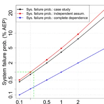
cases of complete dependence (blue) and independence (red) are also provided for comparison. For the case of complete dependence, when the whole region is extreme at the same time, the overall failure probability of the highway is equal to the individual river crossing failure probability. This rep-resents the lowest overall failure probability. The worst case is complete independence where extremes do not happen to-gether unless by random chance; this means that the failure probability of the highway is much higher than that for in-dividual river crossings. Taking into account the real depen-dence, there are some extremes that align, and it seems from Fig. 10 that this is a relatively weak effect. As an example from Fig. 10, to design the highway with a failure probabil-ity of 1 % annual exceedance probabilprobabil-ity (AEP), we would have to design each individual river crossing to a much rarer AEP of 0.25 % (see green lines in Fig. 10).
6 Discussion and conclusions
Hydrological design that is based on IDF estimates has con-ventionally focused on separate estimation at single
loca-tions. Such an approach can lead to the misspecification for a wider system risk of flooding since weather systems exhibit dependence in space and time and across storm durations, which can lead to the coincidence of extremes. A number of methods have been developed to address the problem of antecedent moisture within a single catchment, by account-ing for the temporal dependence of rainfall at locations of interest through loss parameters or sampling rainfall patterns (Rahman et al., 2002). However, there have been fewer meth-ods that account for the spatial dependence of rainfall across multiple catchments, due in part to the complexity of repre-senting the effects of spatial dependence in risk calculations. Different catchments can have different times of concentra-tion, so spatial dependence may also imply the need to con-sider dependence across different durations of extreme rain-fall bursts.
[image:10.612.133.470.262.399.2](Nico-Figure 9.Comparison between conditional flows (red line) and unconditional flows (black line).(a)At the river crossing in the Bellinger catchment (number 1 in Fig. 3): conditional flow caused by a 1-in-10 chance conditional event for 36 h rainfall considering the effect of a 20-year event for 36 h rainfall occurring at the river crossing in the Kalang River catchment, and unconditional flow caused by a 10-year unconditional event for 36 h. (b)At the river crossing in the Deep Creek catchment (number 3 in Fig. 3): conditional flow caused by a 1-in-10 chance conditional event for 9 h rainfall considering the effect of a 20-year event for 36 h rainfall occurring at the river crossing in the Kalang River catchment, and unconditional flow caused by a 10-year unconditional event for 9 h rainfall.
Figure 10.Relationship between system failure probability and in-dividual element failure probability in the percentage of annual ex-ceedance probability (% AEP). Black is for the case study; red is for the case of independence; and blue is for the case of complete dependence. The green lines help to interpolate the individual ele-ment failure probability from a given system failure probability of 1 %. Both the horizontal axis and vertical axis are constructed at a double log scale for viewing purposes.
let et al., 2017; Padoan et al., 2010; Russell et al., 2016; Thibaud et al., 2013; Westra and Sisson, 2011), and latent-variable Gaussian models (Bennett et al., 2016b). The abil-ity to simulate rainfall over a region means that hydrologi-cal problems need not be confined to individual catchments, but they may cover multiple catchments. Civil infrastructure systems such as highways, railways, or levees are such ex-amples, since the failure of any one element may lead to the overall failure of the system. Alternatively, where there is a network, the failure of one element may have implications for the overall system to accommodate the loss, by consid-ering alternative routes. With models of spatial dependence
and the duration dependence of extremes, there is a new and improved ability to address these problems explicitly as part of the design methodology.
This paper demonstrated an application for evaluating con-ditional and joint probabilities of flooding at different loca-tions. This was achieved with two examples: (i) the design of a river crossing that will fail once on average everyMtimes given that its neighboring river crossing is flooded and (ii) the estimation of the probability that a highway section, which contains multiple river crossings, will fail based on the failure probability of each individual river crossing. Due to the lack of continuous streamflow data and sub-daily limitations of rain-based continuous simulation, this study used an event-based method of conditional and joint rainfall extremes to estimate the corresponding conditional and joint flood flows. The spatial rainfall was simulated using an asymptotically independent model, which was then used to estimate con-ditional and joint rainfall extremes. Although this study fo-cused on the inverted max-stable model to simulate the ex-treme rainfall process, other methods such as the Gaussian copula may also be appropriate and should be considered in future applications.
[image:11.612.81.251.286.456.2]related to the ratio of conditional and unconditional rainfall extremes (Fig. 9).
The joint probability of rainfall extremes for all catch-ments and for all possible pairs of catchcatch-ments in the case study area was estimated empirically from a set of 10 000 years of simulated rainfall extremes, repeated 100 times to estimate the average value. The results showed that there were differences in the failure probability of the high-way after taking into account the rainfall dependence, but the effect was not as emphatic as with the case of condi-tional probabilities. The difference in the failure probability became weaker as the return period increased, which is con-sistent with the characteristic of asymptotically independent data (Ledford and Tawn, 1996; Wadsworth and Tawn, 2012). A relationship was demonstrated (Fig. 10) to show how the design of the overall system to a given failure probability re-quires the design of each individual river crossing to a rarer extremal level than when each crossing is considered in iso-lation. For the case study example, it would be necessary to design each of the five bridges to a 0.25 % AEP event in order to obtain a system failure probability of 1 %.
There is a need to reimagine the role of intensity– duration–frequency relationships. Conventionally they have been developed as maps of the marginal rainfall in a point-wise manner for all locations and for a range of frequencies and durations. The increasing sophistication of mathemati-cal models for extremes, computational power, and interac-tive graphics abilities of online mapping platforms means that analysis of hydrological extremes could significantly ex-pand in scope. With an underlying model of spatial and du-ration dependence between the extremes, it is not difficult to conceive of digital maps that dynamically transform from the marginal representation of extremes to the correspond-ing representation conditional extremes after any number of conditions are applied. This transformation is exemplified by the differences between panels a and b in Figs. 7 and 8. En-hanced IDF maps would enable a very different paradigm of design flood risk estimation, breaking away from analyzing individual system elements in isolation and instead empha-sizing the behavior of the entire system.
Table A1.Observed data,Z1andZ2, and corresponding empirical cumulative probabilities,P1andP2.
Z1 Z2 P1 P2
5 10 0.455 0.909
9 1 0.818 0.091
1 7 0.091 0.636
2 6 0.182 0.545
10 4 0.909 0.364
3 3 0.273 0.273
8 9 0.727 0.818
6 2 0.545 0.182
4 8 0.364 0.727
7 5 0.636 0.455
Appendix A: Calculation of the empirical tail dependence coefficient
To illustrate how Eq. (2) in the paper is calculated, consider a set ofn=10 observed values at the two locationsZ1andZ2 (see Table A1). First,Z1andZ2are converted to empirical cumulative probability estimates via the Weibull plotting po-sition formulaP =j/(n+1), wherej is a ranked index of a data point givingP1andP2(see Table A1).
Assume that interest is in values above a thresholdu satis-fyingPu=0.5, in other words,P{Z2> u} =P{P2> Pu} =
0.5. In this case we have only one pair, at the index of 7, that satisfies both P1 andP2 and is greater thanPu=0.5, thus
P{Z1> u, Z2> u} =P{P1> Pu, P2> Pu} =1/10=0.1.
The calculation of the empirical tail dependence coefficient is then
η (x1, x2)= logP{Z2> u}
logP{Z1> u, Z2> u}
= logP{P2> Pu}
logP{P1> Pu, P2> Pu} =log(0.5)
log(0.1)=0.301. (A1)
Appendix B: Estimate of conditional and joint probabilities of rainfall extremes
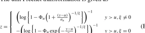
The unit Fréchet transformation is given as
z= log
1−8u
1+(y−u)
σu
−1/ξ−1
y > u, ξ6=0
−
log
1−8uexp
−y−u
σu
−1/ξ−1
y > u, ξ=0
−{logF (yi)}−1 y≤u,
(B1)
whereyis the original marginal value,zis the Fréchet trans-formed value, and all other parameters correspond to the GPD specified in Sect. 4.1. For values below the thresh-old, F is the empirical distribution function ofy,F (yi)=
i/(n+1), whereiis the rank ofyi andnis the total number
of data points.
The conditional probability P{Z2> z2|Z1> z1} is ob-tained from the bivariate inverted max-stable-process cumu-lative distribution function (CDF) in unit Fréchet margins (Thibaud et al., 2013), which is given as
P{Z1≤z1, Z2≤z2}=1−exp
−1 g1 −exp −1 g2 +exp
−V{g1, g2}
, (B2)
where g1= −1/log{1−exp(−1/z1)}, g2= −1/log{1− exp(−1/z2)}, and the exponent measure V (Padoan et al., 2010) is defined as
V{g1, g2} = − 1 g1 8 a 2 + 1 alog g2 g1 − 1 g2 8 a 2+ 1 alog g1 g2 . (B3)
In Eq. (B3),8is the standard normal cumulative distribution function,a=√2γad.(h), and γad.(h) is the variogram that
was mentioned in the explanation of Eq. (3).
In unit Fréchet margins, the relationship between the re-turn levelzand the return periodT (in number of observa-tions) is given asz= −1/log(1−1/T ), and the conditional probability for the max-stable process can then be estimated using
P{Z2> z2|Z1> z1} =T1
1
T1−exp
−1
z2
+P{Z1≤z1, Z2≤z2}], (B4) whereT1is the return period (in number of observations for 36 h rainfall) corresponding to the return levelz1. It is also noted that in this paperZ1andZ2 were taken as threshold exceedances, so the return periodT1should be in the number of observations, which is equivalent to aT1/243-year return period because there are 243 observations for 36 h rainfalls in a year.
The probability that there is at least one location that has an extreme event exceeding a given threshold can be calcu-lated based on the addition rule for the union of probabilities as
P (Z1> z1or. . .orZN> zN)= N
X
i=1
P (Zi> zi)
−X
i<j
P Zi > zi, Zj> zj
+. . .
+(−1)N−1P (Z1> z1,|, . . . , ZN> zN) , (B5)
whereNis the number of locations.
process in Eq. (B2). However, for the case of multiple loca-tions (five different localoca-tions for this paper), it is difficult to derive the formula for this probability because there are de-pendences between extreme events at all locations. So this probability is empirically calculated from a large number of simulations of the dependent model (see the description of the simulation procedure for an inverted max-stable process in Sect. 4.3).
For the case that all the events are independent, the joint probability for independent variables is broken down as the product of the marginals, and the conditional probabil-ity is equivalent to the marginal probabilprobabil-ity. When apply-ing Eq. (B5) for independent variables, the joint probabil-ity is therefore calculated by P (Z1> z1, . . . ,ZN> zN)=
Supplement. The supplement related to this article is available on-line at: https://doi.org/10.5194/hess-23-4851-2019-supplement.
Author contributions. PDL implemented and developed the ap-proach, visualized and interpreted results, and prepared the paper. ML and SW supervised the research and helped to evaluate the methodology and results and edit the paper.
Competing interests. The authors declare that they have no conflict of interest.
Acknowledgements. The lead author was supported by the Aus-tralia Awards Scholarships (AAS) from the AusAus-tralian government. Seth Westra was supported by an Australian Research Council Dis-covery Project (grant no. DP150100411). We thank Mark Babister and Isabelle Testoni of WMA Water for providing the hydrologic models for the case study and Leticia Mooney for her editorial help in improving this paper. The rainfall data used in this study were provided by the Australian Bureau of Meteorology and can be ob-tained from the corresponding author.
Financial support. This research has been supported by the Aus-tralia Awards Scholarships (grant no. DP150100411).
Review statement. This paper was edited by Albrecht Weerts and reviewed by Joost Beckers and two anonymous referees.
References
Ball, J., Babister, M., Nathan, R., Weeks, W., Weinmann, E., Re-tallick, M., and Testoni, I.: Australian Rainfall and Runoff: A Guide to Flood Estimation, ©Commonwealth of Aus-tralia (Geoscience AusAus-tralia), available at: http://book.arr.org.au. s3-website-ap-southeast-2.amazonaws.com/ (last access: 25 Oc-tober 2019), 2016.
Bárdossy, A. and Pegram, G. G. S.: Copula based multisite model for daily precipitation simulation, Hydrol. Earth Syst. Sci., 13, 2299–2314, https://doi.org/10.5194/hess-13-2299-2009, 2009. Baxevani, A. and Lennartsson, J.: A spatiotemporal
precipitation generator based on a censored latent Gaussian field, Water Resour. Res., 51, 4338–4358, https://doi.org/10.1002/2014WR016455, 2015.
Bennett, B., Lambert, M., Thyer, M., Bates, B. C., and Leonard, M.: Estimating Extreme Spatial Rainfall Intensities, J. Hydrol. Eng., 21, 04015074, https://doi.org/10.1061/(ASCE)HE.1943-5584.0001316, 2016a.
Bennett, B., Thyer, M., Leonard, M., Lambert, M., and Bates, B.: A comprehensive and systematic evaluation framework for a parsi-monious daily rainfall field model, J. Hydrol., 556, 1123–1138, https://doi.org/10.1016/j.jhydrol.2016.12.043, 2016b.
Bernard, M. M.: Formulas for rainfall intensities of long duration, T. Am. Soc. Civ. Eng., 96, 592–606, 1932.
Blanchet, J. and Creutin, J.-D.: Co-Occurrence of Extreme Daily Rainfall in the French Mediterranean Region, Water Resour. Res., 53, 9330–9349, https://doi.org/10.1002/2017wr020717, 2017.
Boughton, W., and Droop, O.: Continuous simulation for design flood estimation – a review, Environ. Model. Softw., 18, 309– 318, https://doi.org/10.1016/S1364-8152(03)00004-5, 2003. Boyd, M. J., Rigby, E. H., and VanDrie, R.: WBNM – a
computer software package for flood hydrograph studies, En-vironm. Softw., 11, 167–172, https://doi.org/10.1016/S0266-9838(96)00042-1, 1996.
Cameron, D. S., Beven, K. J., Tawn, J., Blazkova, S., and Naden, P.: Flood frequency estimation by continuous simulation for a gauged upland catchment (with uncertainty), J. Hydrol., 219, 169–187, https://doi.org/10.1016/S0022-1694(99)00057-8, 1999.
Carreau, J., Neppel, L., Arnaud, P., and Cantet, P.: Extreme Rainfall Analysis at Ungaug ed Sites in the South of France: Comparison of Three Approaches, Jour nal de la Société Française de Statis-tique, 154, 119–138, 2013.
Chow, V. T., Maidment, D. R., and Mays, L. W.: Applied Hydrol-ogy, McGraw-Hill, New York, 1988.
Coles, S.: An Introduction to Statistical Modeling of Extreme Val-ues, in: Springer Series in Statistics, Springer, London, 2001. Coles, S., Heffernan, J., and Tawn, J.: Dependence
Mea-sures for Extreme Value Analyses, Extremes, 2, 339–365, https://doi.org/10.1023/a:1009963131610, 1999.
Davison, A. C. and Smith, R. L.: Models for exceedances over high thresholds, J. Roy. Stat. Soc. B, 52, 393–442, 1990.
Davison, A. C., Padoan, S. A., and Ribatet, M.: Statisti-cal Modeling of Spatial Extremes, Stat. Sci., 27, 161–186, https://doi.org/10.1214/11-STS376, 2012.
de Haan, L.: A Spectral Representation for Max-stable Processes, Ann. Probabil., 12, 1194–1204, 1984.
Demarta, S. and McNeil, A. J.: The t Copula and Related Copulas, International Statistical Review/Revue Internationale de Statis-tique, 73, 111–129, 2005.
Dombry, C., Engelke, S., and Oesting, M.: Exact simulation of max-stable processes, Biometrika, 103, 303–317, 2016.
Durocher, M., Chebana, F., and Ouarda, T. B. M. J.: On the prediction of extreme flood quantiles at ungauged locations with spatial copula, J. Hydrol., 533, 523-532, https://doi.org/10.1016/j.jhydrol.2015.12.029, 2016.
Favre, A. C., Adlouni, S. E., Perreault, L., Thiémonge, N., and Bobée, B.: Multivariate hydrological frequency analysis using copulas, Water Resour. Res., 40, W01101, https://doi.org/10.1029/2003WR002456, 2004.
Gupta, A. S. and Tarboton, D. G.: A tool for downscaling weather data from large-grid reanalysis products to finer spatial scales for distributed hydrological applications, Environ. Model. Softw., 84, 50-69, https://doi.org/10.1016/j.envsoft.2016.06.014, 2016. He, Y., Bárdossy, A., and Zehe, E.: A review of regionalisation for
continuous streamflow simulation, Hydrol. Earth Syst. Sci., 15, 3539–3553, https://doi.org/10.5194/hess-15-3539-2011, 2011. Hegnauer, M., Beersma, J., Van den Boogaard, H., Buishand, T.,
http://publications.deltares.nl/1209424_004_0018.pdf (last ac-cess: 25 October 2019), 2014.
Hosking, J. R. M. and Wallis, J. R.: Regional Frequency Analy-sis – An Approach Based on L-Moments, Cambridge University Press, Cambridge, UK, 1997.
Hüsler, J. and Reiss, R.-D.: Maxima of normal random vectors: Be-tween independence and complete dependence, Stat. Probabil. Lett., 7, 283–286, https://doi.org/10.1016/0167-7152(89)90106-5, 1989.
Kao, S.-C. and Govindaraju, R. S.: Trivariate statisti-cal analysis of extreme rainfall events via the Plack-ett family of copulas, Water Resour. Res., 44, W02415, https://doi.org/10.1029/2007WR006261, 2008.
Kleiber, W., Katz, R. W., and Rajagopalan, B.: Daily spa-tiotemporal precipitation simulation using latent and trans-formed Gaussian processes, Water Resour. Res., 48, W01523, https://doi.org/10.1029/2011WR011105, 2012.
Koutsoyiannis, D., Kozonis, D., and Manetas, A.: A math-ematical framework for studying rainfall intensity-duration-frequency relationships, J. Hydrol., 206, 118–135, https://doi.org/10.1016/S0022-1694(98)00097-3, 1998. Kuichling, E.: The relation between the rainfall and the discharge
of sewers in populous districts, T. Am. Soc. Civ. Eng., 20, 1–56, 1889.
Laurenson, E. M. and Mein, R. G.: RORB Version 4 Runoff Routing Program User Manual, Monash University Department of Civil Engineering, Clayton, Victoria, 1990.
Le, P. D., Davison, A. C., Engelke, S., Leonard, M., and Westra, S.: Dependence properties of spatial rainfall ex-tremes and areal reduction factors, J. Hydrol., 565, 711–719, https://doi.org/10.1016/j.jhydrol.2018.08.061, 2018a.
Le, P. D., Leonard, M., and Westra, S.: Modeling Spa-tial Dependence of Rainfall Extremes Across Mul-tiple Durations, Water Resour. Res., 54, 2233–2248, https://doi.org/10.1002/2017WR022231, 2018b.
Le, P. D., Leonard, M., and Westra, S.: Spatially dependent flood probabilities to support the design of civil infrastructure systems – Data sets, https://doi.org/10.6084/m9.figshare.9917072.v1, 2019.
Ledford, A. W. and Tawn, J. A.: Statistics for Near Independence in Multivariate Extreme Values, Biometrika, 83, 169–187, 1996. Leonard, M., Lambert, M. F., Metcalfe, A. V., and
Cowpert-wait, P. S. P.: A space-time Neyman–Scott rainfall model with defined storm extent, Water Resour. Res., 44, W09402, https://doi.org/10.1029/2007WR006110, 2008.
Leonard, M., Westra, S., Phatak, A., Lambert, M., v. d. Hurk, B., McInnes, K., Risbey, J., Schuster, S., Jakob, D., and Stafford-Smith, M.: A compound event framework for understanding ex-treme impacts, Wiley Interdisciplin. Rev.: Clim. Change, 5, 113– 128, https://doi.org/10.1002/wcc.252, 2014.
Mulvaney, T. J.: On the use of self-registering rain and flood gauges in making observation of the relation of rainfall and floods dis-charges in a given catchment, Proc. Civ. Eng. Ireland, 4, 18–31, 1851.
Nicolet, G., Eckert, N., Morin, S., and Blanchet, J.: A multi-criteria leave-two-out cross-validation procedure for max-stable process selection, Spat. Stat., 22, 107–128, https://doi.org/10.1016/j.spasta.2017.09.004, 2017.
Padoan, S. A., Ribatet, M., and Sisson, S. A.: Likelihood-Based In-ference for Max-Stable Processes, J. Am. Stat. Assoc., 105, 263– 277, https://doi.org/10.1198/jasa.2009.tm08577, 2010.
Pathiraja, S., Westra, S., and Sharma, A.: Why continu-ous simulation? The role of antecedent moisture in de-sign flood estimation, Water Resour. Res., 48, W06534, https://doi.org/10.1029/2011WR010997, 2012.
Pickands, J.: Statistical Inference Using Extreme Order Statistics, Ann. Stat., 3, 119–131, https://doi.org/10.1214/aos/1176343003, 1975.
Rahman, A., Weinmann, P. E., Hoang, T. M. T., and Laurenson, E. M.: Monte Carlo simulation of flood frequency curves from rain-fall, J. Hydrol., 256, 196–210, https://doi.org/10.1016/S0022-1694(01)00533-9, 2002.
Rasmussen, P. F.: Multisite precipitation generation using a la-tent autoregressive model, Water Resour. Res., 49, 1845–1857, https://doi.org/10.1002/wrcr.20164, 2013.
Renard, B. and Lang, M.: Use of a Gaussian copula for multivariate extreme value analysis: Some case stud-ies in hydrology, Adv. Water Resour., 30, 897–912, https://doi.org/10.1016/j.advwatres.2006.08.001, 2007. Requena, A. I., Chebana, F., and Ouarda, T. B. M. J.: A
func-tional framework for flow-duration-curve and daily streamflow estimation at ungauged sites, Adv. Water Resour., 113, 328–340, https://doi.org/10.1016/j.advwatres.2018.01.019, 2018. Russell, B. T., Cooley, D. S., Porter, W. C., and Heald,
C. L.: Modeling the spatial behavior of the meteorological drivers’ effects on extreme ozone, Environmetrics, 27, 334–344, https://doi.org/10.1002/env.2406, 2016.
Schlather, M.: Models for Stationary Max-Stable Random Fields, Extremes, 5, 33–44, https://doi.org/10.1023/A:1020977924878, 2002.
Seneviratne, S. I., Nicholls, N., Easterling, D., Goodess, C. M., Kanae, S., Kossin, J., Luo, Y., Marengo, J., McInnes, K., and Rahimi, M.: Managing the Risks of Extreme Events and Disas-ters to Advance Climate Change Adaptation: Changes in Climate Extremes and their Impacts on the Natural Physical Environ-ment, Cambridge University Press, Cambridge, UK, 109–230, 2012.
SKM: Nambucca Heads Flood Study, available at: http://www. nambucca.nsw.gov.au/cp_content/resources/16152_2011_ _Nambucca_Heads_Flood_Study_Final_Draft_Chapter_6a.pdf (last access: 25 October 2019), 2011.
Stedinger, J., Vogel, R., and Foufoula-Georgiou, E.: Frequency Analysis of Extreme Events, in: Handbook of Hydrology, edited by: Maidment, D. R., McGraw-Hill, New York, 18.11–18.66, 1993.
Stephenson, A. G., Lehmann, E. A., and Phatak, A.: A max-stable process model for rainfall extremes at different ac-cumulation durations, Weather Clim. Extrem., 13, 44–53, https://doi.org/10.1016/j.wace.2016.07.002, 2016.
Thibaud, E., Mutzner, R., and Davison, A. C.: Threshold modeling of extreme spatial rainfall, Water Resour. Res., 49, 4633–4644, https://doi.org/10.1002/wrcr.20329, 2013.
Wang, Q. J.: A Bayesian Joint Probability Approach for flood record augmentation, Water Resour. Res., 37, 1707–1712, https://doi.org/10.1029/2000WR900401, 2001.
Wang, Q. J., Robertson, D. E., and Chiew, F. H. S.: A Bayesian joint probability modeling approach for seasonal forecasting of streamflows at multiple sites, Water Resour. Res., 45, W05407, https://doi.org/10.1029/2008WR007355, 2009.
Wang, X., Gebremichael, M., and Yan, J.: Weighted likelihood copula modeling of extreme rainfall events in Connecticut, J. Hydrol., 390, 108–115, https://doi.org/10.1016/j.jhydrol.2010.06.039, 2010.
Westra, S. and Sisson, S. A.: Detection of non-stationarity in pre-cipitation extremes using a max-stable process model, J. Hydrol., 406, 119–128, https://doi.org/10.1016/j.jhydrol.2011.06.014, 2011.
WMAWater: Review of Bellinger, Kalang and Nambucca River Catchments Hydrology, Bellingen Shire Council, Nambucca Shire Council, New South Wales Government, 2011.
Zhang, L. and Singh, V. P.: Gumbel 2013; Hougaard Cop-ula for Trivariate Rainfall Frequency Analysis, J. Hy-drol. Eng., 12, 409–419, https://doi.org/10.1061/(ASCE)1084-0699(2007)12:4(409), 2007.
Zheng, F., Westra, S., and Leonard, M.: Opposing local precipitation extremes, Nat. Clim. Change, 5, 389–390, https://doi.org/10.1038/nclimate2579, 2015.