https://doi.org/10.5194/hess-23-3503-2019 © Author(s) 2019. This work is distributed under the Creative Commons Attribution 4.0 License.
Trajectories of nitrate input and output in three nested catchments
along a land use gradient
Sophie Ehrhardt1, Rohini Kumar2, Jan H. Fleckenstein1,3, Sabine Attinger2, and Andreas Musolff1
1Department of Hydrogeology, Helmholtz-Centre for Environmental Research, 04318 Leipzig, Germany
2Department Computational Hydrosystems, Helmholtz-Centre for Environmental Research, 04318 Leipzig, Germany 3Bayreuth Center of Ecology and Environmental Research, University of Bayreuth, 95440 Bayreuth, Germany
Correspondence:Sophie Ehrhardt ([email protected]) Received: 6 September 2018 – Discussion started: 22 October 2018
Revised: 20 June 2019 – Accepted: 6 July 2019 – Published: 2 September 2019
Abstract.Increased anthropogenic inputs of nitrogen (N) to the biosphere during the last few decades have resulted in increased groundwater and surface water concentrations of N (primarily as nitrate), posing a global problem. Although measures have been implemented to reduce N inputs, they have not always led to decreasing riverine nitrate concentra-tions and loads. This limited response to the measures can ei-ther be caused by the accumulation of organic N in the soils (biogeochemical legacy) – or by long travel times (TTs) of inorganic N to the streams (hydrological legacy). Here, we compare atmospheric and agricultural N inputs with long-term observations (1970–2016) of riverine nitrate concentra-tions and loads in a central German mesoscale catchment with three nested subcatchments of increasing agricultural land use. Based on a data-driven approach, we assess jointly the N budget and the effective TTs of N through the soil and groundwater compartments. In combination with long-term trajectories of theC–Qrelationships, we evaluate the poten-tial for and the characteristics of an N legacy.
We show that in the 40-year-long observation period, the catchment (270 km2) with 60 % agricultural area received an N input of 53 437 t, while it exported 6592 t, indicating an overall retention of 88 %. Removal of N by denitrification could not sufficiently explain this imbalance. Log-normal travel time distributions (TTDs) that link the N input his-tory to the riverine export differed seasonally, with modes spanning 7–22 years and the mean TTs being systematically shorter during the high-flow season as compared to low-flow conditions. Systematic shifts in theC–Qrelationships were noticed over time that could be attributed to strong changes in N inputs resulting from agricultural intensification before
1989, the break-down of East German agriculture after 1989 and the seasonal differences in TTs. A chemostatic export regime of nitrate was only found after several years of sta-bilized N inputs. The changes inC–Qrelationships suggest a dominance of the hydrological N legacy over the biogeo-chemical N fixation in the soils, as we expected to observe a stronger and even increasing dampening of the riverine N concentrations after sustained high N inputs. Our analyses reveal an imbalance between N input and output, long time-lags and a lack of significant denitrification in the catchment. All these suggest that catchment management needs to ad-dress both a longer-term reduction of N inputs and shorter-term mitigation of today’s high N loads. The latter may be covered by interventions triggering denitrification, such as hedgerows around agricultural fields, riparian buffers zones or constructed wetlands. Further joint analyses of N budgets and TTs covering a higher variety of catchments will pro-vide a deeper insight into N trajectories and their controlling parameters.
1 Introduction
N fixation and the internal combustion engine (Elser, 2011). Therefore the amount of reactive N that enters into the el-ement’s biospheric cycle has been doubled in comparison to the preindustrial era (Smil, 1999; Vitousek et al., 1997). However, the different input sources of N show diverging rates of change over time and space. While the atmospheric emissions of N oxides and ammonia have strongly declined in Europe since the 1980s (EEA, 2014), the agricultural N input through fertilizers declined but is still at a high level (Federal Ministry for the Environment and Federal Ministry of Food, 2012). In the cultural landscape of western coun-tries, most of the N emissions in surface and groundwater bodies stem from diffuse agricultural sources (Bouraoui and Grizzetti, 2011; Dupas et al., 2013).
The widespread consequences of these excessive N puts are significantly elevated concentrations of dissolved in-organic nitrogen (DIN) in groundwater and connected sur-face waters (Altman and Parizek, 1995; Sebilo et al., 2013; Wassenaar, 1995), leading to increased riverine DIN fluxes (Dupas et al., 2016) and causing the ecological degradation of freshwater and marine systems. This degradation is caused by the ability of N species to increase primary production and to change food web structures (Howarth et al., 1996; Turner and Rabalais, 1991). In particular, the coastal marine envi-ronments, where nitrate (NO3) is typically the limiting
nutri-ent, are affected by these eutrophication problems (Decrem et al., 2007; Prasuhn and Sieber, 2005).
Several initiatives in the form of international, national and federal regulations have been implemented, aiming at an overall reduction of N inputs into the terrestrial system and its transfer to the aquatic system. In the European Union, guidelines are provided to its member states for national pro-grams of measures and evaluation protocols through the Ni-trate Directive (CEC, 1991) and the Water Framework Direc-tive (CEC, 2000).
The evaluation of interventions showed that policy-makers still struggle to set appropriate goals for water quality im-provement, particularly in heavily human-impacted water-sheds. Studies in Europe and the United States showed that interventions like reduced N inputs mainly in agricul-tural land use do not immediately result in declining river-ine NO3–N concentrations (Bouraoui and Grizzetti, 2011;
Sprague et al., 2011; Howden et al., 2011) and fluxes (Wor-rall et al., 2009), although fast responding headwaters have been reported as well (Rozemeijer et al., 2014).
In Germany considerable progress has been achieved in the improvement of water quality, but the diffuse water pol-lution from agricultural sources continues to be of concern (Wendland et al., 2005). This limited response to mitigation measures can partly be explained by nutrient legacy effects, which stem from an accumulation of excessive fertilizer in-puts over decades creating a strongly dampened response between the implementation of measures and water quality improvement (van Meter and Basu, 2015). Furthermore, the multi-year travel times (TTs) of nitrate through the soil and
groundwater compartments cause large time lags (Howden et al., 2010; Melland et al., 2012) that can substantially delay the riverine response to applied management interventions. For a targeted and effective water quality management, we therefore need a profound understanding of the processes and controls of time lags of N from the source to groundwater and surface water bodies. Bringing together N balancing and accumulation with estimations of N TTs from application to riverine exports can contribute to this lack of knowledge.
Estimation of the water or solute TTs is essential for pre-dicting the retention, mobility and fate of solutes, nutrients and contaminants at catchment scale (Jasechko et al., 2016). Time series of solute concentrations and loads that cover both input to the geosphere and the subsequent riverine ex-port can be used not only to determine TTs (van Meter and Basu, 2017), but also to quantify mass losses in the export as well as the behavior of the catchment’s retention capac-ity (Dupas et al., 2015). Knowledge on the TT of N would therefore allow understanding on the N transport behavior, defining the fate of injected N mass into the system and its contribution to riverine N response. The mass of N being transported through the catchment storage can be referred to as hydrological legacy. Data-driven or simplified mechanis-tic approaches have often been used to derive stationary and seasonally variable travel time distributions (TTDs) using in-put and outin-put signals of conservative tracers or isotopes (Jasechko et al., 2016; Heidbüchel et al., 2012) or chloride concentrations (Kirchner et al., 2000; Bennettin et al., 2015). Recently, van Meter and Basu (2017) estimated the solute TTs for N transport at several stations across a catchment located in Southern Ontario, Canada, showing decadal time-lags between input and riverine exports. Moreover, system-atic seasonal variations in the NO3–N concentrations have
been found, which were explained by seasonal shifts in the N delivery pathways and connected time lags (van Meter and Basu, 2017). Despite the determination of such sea-sonal concentration changes and age dynamics, there are rel-atively few studies focussing on their long-term trajectory under conditions of changing N inputs (Dupas et al., 2018; Howden et al., 2010; Minaudo et al., 2015; Abbott et al., 2018). Seasonally differing time shifts, resulting in chang-ing intra-annual concentration variations are of importance to aquatic ecosystems’ health and their functionality. Sea-sonal concentration changes can also be directly connected to changing concentration–discharge (C–Q) relationships – a tool for classifying observed solute responses to changing discharge conditions and for characterizing and understand-ing anthropogenic impacts on solute input, transport and fate (Jawitz and Mitchell, 2011; Musolff et al., 2015). Investiga-tions of temporal dynamics in the C–Q relationship are a valuable addition to approaches based on N balancing only (e.g., Abbott et al., 2018), when evaluating the effect of man-agement interventions.
ln(C)–ln(Q) regression (Godsey et al., 2009): with enrich-ment (b >0), dilution (b <0) or constant (b ≈0) patterns (Musolff et al., 2017). On the other hand, C–Q relation-ships can be classified according to the ratio between the coefficients of variation of concentration (CVC) and of dis-charge (CVQ; Thompson et al., 2011). This export regime can be either chemodynamic (CVC/CVQ>0.5) or chemo-static, where the variance of the solute load is more domi-nated by the variance in discharge than the variance in con-centration (Musolff et al., 2017). Both patterns and regimes are dominantly shaped by the spatial distribution of solute sources (Seibert et al., 2009; Basu et al., 2010; Thompson et al., 2011; Musolff et al., 2017). High source heterogeneity and consequently high concentration variability is thought to be characteristic for nutrients under pristine conditions (Mu-solff et al., 2017; Basu et al., 2010). It was shown in Germany and the United States that catchments under intensive agri-cultural use evolve from chemodynamic to more chemostatic behavior regarding nitrate export (Thompson et al., 2011; Dupas et al., 2016). Several decades of human N inputs seem to dampen the discharge-dependent concentration variabil-ity, resulting in chemostatic behavior, where concentrations are largely independent of discharge variations (Dupas et al., 2016). Also Thompson et al. (2011) stated observational and model-based evidence of an increasing chemostatic response of nitrate with increasing agricultural intensity. This shift in the export regimes is caused by a long-term homogenization of the nitrate sources in space and/or at depth within soils and aquifers (Dupas et al., 2016; Musolff et al., 2017). However, effective denitrification in the subsurface can create concen-tration variability over depths and flow path age and thus has been shown to result in chemodynamic exports even with in-tensive agriculture (van der Velde et al., 2010; Musolff et al., 2017). Long-term N inputs lead to a loading of all flow paths in the catchment with mobile fractions of N and by that the formation of a hydrological N legacy (van Meter and Basu, 2015) and chemostatic riverine N exports. On the other hand, excessive fertilizer input is linked to the above-mentioned buildup of legacy N stores in the catchment, changing the export regime from a supply- to a transport-limited chemo-static one (Basu et al., 2010). This legacy is manifested as a biogeochemical legacy in the form of increased, less mobile, organic N content within the soil (Worral et al., 2015; van Meter and Basu, 2015; van Meter et al., 2017a). This type of legacy buffers biogeochemical variations, so that man-agement measures can only show their effect if the buildup source gets substantially depleted (Basu et al., 2010).
Depending on the catchment configuration, both forms of legacy – hydrological and biogeochemical – can exist with different shares of the total N stored in a catchment (van Me-ter et al., 2017a). However, biogeochemical legacy is hard to distinguish from hydrological legacy when looking at time lags between N input and output or at catchment-scale N budgets only (van Meter and Basu, 2015). One way to better disentangle the N legacy types is applying the framework of
C–Qrelationships as defined by Jawitz and Mitchell (2011) and Musolff et al. (2015, 2017). In the case of a hydrological legacy, strong changes in fertilizer inputs (such as increasing inputs in the initial phase of intensification and decreasing inputs as a consequence of measures) will temporarily in-crease spatial concentration heterogeneity (e.g., comparing young and old water fractions in the catchment storage), and therefore also shift the export regime to more chemodynamic conditions. On the other hand, a dominant biogeochemical legacy will lead to sustained concentration homogeneity in the N source zone in the soils and to an insensitivity of the riverine N export regime to fast changes in inputs.
Common approaches to quantify catchment-scale N bud-gets and to characterize legacy or to derive TTs are either based on data-driven (Worral et al., 2015; Dupas et al., 2016) or on forward-modeling (van Meter and Basu, 2015; van Me-ter et al., 2017a) approaches. So far, data-driven studies fo-cused either solely on N budgeting and legacy estimation or on TTs. Here, we conducted a joint data-driven assessment of the catchment-scale N budget, the potential and charac-teristics of an N legacy, and the estimation of TTs of the riverine exported N. We utilized the trajectory of agricultural catchments in terms ofC–Qrelationships, their changes over longer timescales and their potential evolution to a chemo-static export regime. The novel combination of the long-term N budgeting, TT estimation and C–Q trajectory will help understanding of the differentiation between biogeochemical and hydrological legacy, both reasons for missed targets in water quality management. This study will address the fol-lowing research questions:
1. How high is the retention potential for N of the studied mesoscale catchment and what are the consequences in terms of a potential buildup of an N legacy?
2. What are the characteristics of the TTD for N that links change in the diffuse anthropogenic N inputs to the geo-sphere and their observable effect in riverine NO3–N
concentrations?
3. What are the characteristics of a long-term trajectory of C–Qrelationships? Is there an evolution to a chemo-static export regime that can be linked to a biogeochem-ical or hydrologbiogeochem-ical N legacy?
for many mesoscale catchments in Germany and elsewhere. Moreover, this catchment offers a unique possibility to ana-lyze the system response to strong changes in fertilizer usage in East Germany before and after reunification. Thereby, we anticipate that our improved understanding gained through this study in these catchment settings is transferable to sim-ilar regions. In comparison to spatially and temporally inte-grated water quality signals stemming solely from the catch-ment outlet, the higher spatial resolution with three stations and the unique length of the monitoring period (1970–2016) allow for a more detailed investigation about the fate of N, and consequently findings may provide guidance for effec-tive water quality management.
2 Data and methods 2.1 Study area
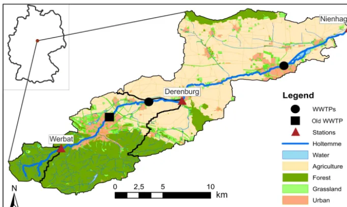
The Holtemme catchment (270 km2) is a subcatchment of the Bode River basin, which is part of the TERENO (TER-restrial ENvironmental Observatories) Harz/Central German Lowland Observatory (Fig. 1). The catchment, as part of the TERENO project, exhibits strong gradients in topography, climate, geology, soils, water quality, land use and level of urbanization (Wollschläger et al., 2017). Due to the low wa-ter availability and the risk of summer droughts that might be further exacerbated by a decrease in summer precipi-tation and increased evaporation with rising temperatures, the region is ranked as highly vulnerable to climate change (Schröter et al., 2005; Samaniego et al., 2018). With these conditions, the catchment is representative of other German and central European regions showing similar vulnerability (Zacharias et al., 2011). The observatory is one of the mete-orologically and hydrologically best-equipped catchments in Germany (Zacharias et al., 2011; Wollschläger et al., 2017) and provides long-term data for many environmental vari-ables including water quantity (e.g., precipitation, discharge) and water quality at various locations.
The Holtemme catchment has its spring at 862 m a.s.l. in the Harz Mountains and extends to the northeast to the cen-tral German lowlands with an outlet at 85 m a.s.l. The long-term annual mean precipitation (1951–2015) shows a re-markable decrease from a colder and humid climate in the Harz Mountains (1262 mm) down to the warmer and dryer climate of the central German lowlands on the leeward side of the mountains (614 mm; Rauthe et al., 2013; Frick et al., 2014). Discharge time series, provided by the State Of-fice of Flood Protection and Water Management (LHW) of Saxony-Anhalt show a mean annual discharge at the outlet in Nienhagen of 1.5 m3s−1(1976–2016), corresponding to 172 mm a−1.
The geology of the catchment is dominated by late Paleo-zoic rocks in the mountainous upstream part that are largely covered by Mesozoic rocks as well as Tertiary and
Quater-nary sediments in the lowlands (Frühauf and Schwab, 2008; Schuberth, 2008). Land use of the catchment changes from forests in the pristine, mountainous headwaters to intensive agricultural use in the downstream lowlands (EEA, 2012). According to Corine Land Cover (CLC) from different years (1990, 2000, 2006, 2012), the land use change over the inves-tigated period is negligible. Overall 60 % of the catchment is used for agriculture, with a crop rotation of wheat, barley, triticale, rye and rapeseed (Yang et al., 2018b), while 30 % is covered by forest (EEA, 2012). Urban land use occupies 8 % of the total catchment area (EEA, 2012) with two major towns (Wernigerode, Halberstadt) and several small villages. Two wastewater treatment plants (WWTPs) discharge into the river. The town of Wernigerode had its WWTP within its city boundaries until 1995, when a new WWTP was put into operation about 9.1 km downstream in a smaller vil-lage, called Silstedt, replacing the old WWTP. The WWTP in Halberstadt was not relocated but renovated in 2000. Nowadays, the total nitrogen load (TNb) in cleaned water is approximately 67.95 kg d−1 (WWTP Silstedt: NO3–N load
55 kg d−1) and 35.09 kg d−1 (WWTP Halberstadt: NO3–N
load 6.7 kg d−1; mean daily loads 2014; Müller et al., 2018). Referring to the last 5 years of observations, NO3–N load
from wastewater made up 17 % of the total observed NO3–
N flux at the midstream station (see below) and 11 % at the downstream station. Despite this point source N input, the major nitrate contribution is due to inputs from agricultural land use (Müller et al., 2018), which is predominant in the mid- and downstream part of the catchment (Fig. 1).
Figure 1.Map of the Holtemme catchment with the selected sampling locations. Map created from ATKIS data.
by Chernozems (Schuberth, 2008), representing one of the most fertile soils within Germany (Schmidt, 1995). Hence, the agricultural land use in this subcatchment is the high-est (81 %) in comparison to the two upstream subcatchments (EEA, 2012).
2.2 Nitrogen input
The main N sources were quantified over time, assisting the data-based input–output assessment to address the three re-search questions regarding the N budgeting, effective TTs andC–Qrelationships in the catchment.
A recent investigation in the study catchment by Müller et al. (2018) showed that the major nitrate contribution stems from agricultural land use and the associated application of fertilizers. The quantification of this contribution is the N sur-plus (also referred to as agricultural sursur-plus) that reflects N input that is in excess of crop and forage needs. For Germany there is no consistent dataset available for the N surplus that covers all land use types and is sufficiently resolved in time and space. Therefore, we combined the available agricultural N input (including atmospheric deposition) dataset with an-other dataset of atmospheric N deposition rates for the nona-gricultural land.
The annual agricultural N input for the Holtemme catch-ment was calculated using two different datasets of agri-cultural N surplus across Germany provided by the Univer-sity of Gießen (Bach and Frede, 1998; Bach et al., 2011). Surplus data (kg N ha−1a−1) were available at the federal state level for 1950–2015 and at the county level for 1995– 2015, with an accuracy level of 5 % (see Bach and Frede, 1998, for more details). We used the data from the over-lapping time period (1995–2015) to downscale the state-level data (state: Saxony-Anhalt) to the county state-level (county:
Harzkreis). Both (the state level and the aggregated county to state level) datasets show high correspondence with a corre-lation (R2) of 0.85, but they differ slightly in their absolute values (by 6 % of the mean annual values). The mean offset of 3.85 kg N ha−1a−1was subtracted from the federal state level data to yield the surplus in the county before 1995.
Both of the above datasets account for the atmospheric de-position, but only on agricultural areas. For other nonagricul-tural areas (forest and urban landscapes), the N source stem-ming from atmospheric deposition was quantified based on datasets from the Meteorological Synthesizing Centre – West (MSC-W) of the European Monitoring and Evaluation Pro-gramme (EMEP). The underlying dataset consists of gridded fields of EU-wide wet and dry atmospheric N depositions from a chemical transport model that assimilates different observational records on atmospheric chemicals (e.g., Bart-nicky and Benedictow, 2017; BartBart-nicky and Fagerli, 2006). This dataset is available with annual time-steps since 1995, and with data every 5 years between 1980 and 1995. Data between the 5-year time steps were linearly interpolated to obtain annual estimates of N deposition between 1980 and 1995. For years prior to 1980, we made use of global grid-ded estimates of atmospheric N deposition from the three-dimensional chemistry-transport model (TM3) for the year 1860 (Dentener, 2006; Galloway et al., 2004). In absence of any other information, we performed a linear interpolation of the N deposition estimates between 1860 and 1980.
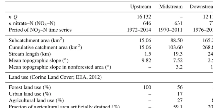
Table 1.General information on the study area, including input–output datasets;n– number of observations,Q– discharge.
Upstream Midstream Downstream
n Q 16 132 – 12 114
nnitrate–N (NO3–N) 646 631 770
Period of NO3–N time series 1972–2014 1970–2011 1976–2016
Subcatchment area (km2) 15.06 88.50 165.22 Cumulative catchment area (km2) 15.06 103.60 268.80
Stream length (km) 1.5 19.3 24.4
Mean topographic slope (◦) 9.82 7.52 2.55 Mean topographic slope in nonforested area (◦) – 3.2 1.9 Land use (Corine Land Cover; EEA, 2012)
Forest land use (%) 100 56 11
Urban land use (%) – 17 8
Agricultural land use (%) – 27 81
Fraction of agricultural area artificially drained (%) – 59.1 20.5
2.7 kg N ha−1a−1, respectively. The atmospheric deposition and biological fixation for the different nonagricultural land uses were added to the agricultural N surplus to achieve the total N input per area. In contrast to the widely applied term net anthropogenic nitrogen input (NANI), we do not account for wastewater fluxes in the N input but rather focus on the diffuse N input and connected flow paths, where legacy accu-mulation and time lags between input and output potentially occur.
2.3 Nitrogen output
2.3.1 Discharge and water quality time series
Discharge and water quality observations were used to quan-tify the N load and to characterize the trajectory of NO3–
N concentrations and theC–Qtrajectories in the three sub-catchments.
The data for water quality (biweekly to monthly) and dis-charge (daily) from 1970 to 2016 were provided by the LHW of Saxony-Anhalt. The biweekly to monthly sampling was done at gauging stations defining the three subcatchments. The datasets cover a wide range of instream chemical con-stituents including major ions, alkalinity, nutrients and in situ measured parameters (pH, O2, water temperature, electrical
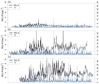
conductivity). As this study only focuses on N species, we restricted the selection of parameters to nitrate (NO3; Fig. 2),
nitrite (NO2; Fig. S1.2.2) and ammonium (NH4; Fig. S1.2.1).
Discharge time series at daily timescales were measured at two of the water quality stations (upstream, downstream; Fig. 2). Continuous daily discharge series are required to calculate flow-normalized concentrations (see the following Sect. 2.3.2 for more details). To derive the discharge data for the midstream station and to fill measurement gaps at the other stations (2 % upstream, 3 % downstream), we used simulations from a grid-based distributed mesoscale
hydro-logical model mHM (Samaniego et al., 2010; Kumar et al., 2013). Daily mean discharge was simulated for the same time frame as the available measured data. We used a model setup similar to Müller et al. (2016) with robust results capturing the observed variability of discharge in the nearby studied catchments. We note that the discharge time series were used as weighting factors in the later analysis of flow-normalized concentrations. Consequently it is more important to capture the temporal dynamics than the absolute values. Nonetheless, we performed a simple bias correction method by applying the regression equation of simulated and measured values to reduce the simulated bias of modeled discharge. After this re-vision, the simulated discharges could be used to fill the gaps of measured data. The midstream station (Derenburg) for the water quality data is 5.6 km upstream of the next gauging station. Therefore, the nearest station (Mahndorf) with simu-lated and measured discharge data was used to derive the bias correction equation that was subsequently applied to correct the simulated discharge data at the midstream station, assum-ing the same bias between modeled and observed discharges at the gauging station.
2.3.2 Weighted regression on time, discharge, and season (WRTDS) and wastewater correction The software package “Exploration and Graphics for RivEr Trends” (EGRET) in the R environment by Hirsch and DeCicco (2019) was used to estimate daily concentrations of NO3–N utilizing “Weighted Regressions on Time,
Figure 2.NO3–N concentration and discharge (Q) time series: upstream(a), midstream(b)and downstream(c).
trend and seasonal component) is fitted for each day of the flow record with a flexible weighting of observations based on their time, seasonal and discharge “distance” (Hirsch et al., 2010). Results are daily concentrations and fluxes as well as daily flow-normalized concentrations and fluxes. Flow normalization uses the probability distribution of discharge of the specific day of the year from the entire discharge time series. More specifically, the flow-normalized concentration is the average of the same regression model for a specific day applied to all measured discharge values of the corre-sponding day of the year. While the non-flow-normalized concentrations are strongly dependent on the discharge, the flow-normalized estimations provide a more unbiased, ro-bust estimate of the concentrations with a focus on changes in concentration and fluxes independent of interannual dis-charge variability (Hirsch et al., 2010). To account for un-certainty in the regression analysis of annual and seasonal flow-normalized concentration and fluxes, we used the block bootstrap method introduced by Hirsch et al. (2015). We de-rived the 5th and 95th percentile of annual flow-normalized concentration and flux estimates with a block length of 200 d and 10 replicates. The results are utilized to communicate uncertainty in both the N budgeting and the resulting TT es-timation.
The study of Müller et al. (2018) indicated the dominance of N from diffuse sources in the Holtemme catchment but also stressed the impact of wastewater-borne nitrate during
low-flow periods. Because our purpose was to balance and compare N input and outputs from diffuse sources only, the provided annual flux of total N from the two WWTPs was therefore used to correct flow-normalized fluxes and con-centrations derived from the WRTDS assessment. We argue that the annual wastewater N flux is robust enough to cor-rect the flow-normalized concentrations, but it does not al-low for the correction of measured concentration data on a specific day. Both treatment plants provided snapshot sam-ples of both NO3–N and total N fluxes to derive the
frac-tion of N that is discharged as NO3–N into the stream. This
fraction is 19 % for the WWTP Halberstadt (384 measure-ments between January 2014 to July 2016) and 81 % for Sil-stedt (eight measurements from February 2007 to Decem-ber 2017). We argue that the fraction of N leaving as NH4,
NO2and Norgdoes not interfere with the NO3–N flux in the
river due to the limited stream length and therefore nitrifica-tion potential of the Holtemme River impacted by wastewa-ter (see also Sect. S1.2.3). We related the wastewawastewa-ter-borne NO3–N flux to the flow-normalized daily flux of NO3–N
from the WRTDS method to get a daily fraction of wastew-ater NO3–N in the river that we used to correct the
that, we assume that wastewater-borne N dominantly leaves the treatment plants as NH4-N (see also Fig. S1.2.1).
Based on the daily resolved flow-normalized and wastewater-corrected concentration and flux data, descriptive statistical metrics were calculated on an annual timescale. Seasonal statistics of each year were also calculated for win-ter (December, January, February), spring (March, April, May), summer (June, July, August) and fall (September, Oc-tober, November). Note that statistics for the winter season incorporate December values from the calendar year before. Following Musolff et al. (2015, 2017), the ratio of CVC/CVQ and the slope (b) of the linear relationship be-tween ln(C) and ln(Q) were used to characterize the export pattern and the export regimes of NO3–N along the three
study catchments.
2.4 Input–output assessment: nitrogen budgeting and effective travel times
The input–output assessment is needed to estimate the re-tention potential for N in the catchment as well as to link temporal changes in the diffuse anthropogenic N inputs to the observed changes in the riverine NO3–N concentrations.
The stream concentration of a given solute, e.g., as shown by Kirchner et al. (2000), is assumed at any time as the convo-lution of the TTD and the rainfall concentration throughout the past. This study applies the same principle for the N input as incoming time series that, when convolved with the TTD, yields the stream concentration time series. We selected a log-normal distribution function (with two parameters,µand σ) as a convolution transfer function, based on a recent study by Musolff et al. (2017), who successfully applied this form of a transfer function to represent TTs. The two free param-eters were obtained through optimization based on minimiz-ing the sum of squared errors between observed and simu-lated N exports. The form of selected transfer function is in line with Kirchner et al. (2000) stating that exponential TTDs are unlikely at catchment scale, but rather a skewed, long-tailed distribution would be likely. Note that we used the log-normal distribution as a transfer function between the tem-poral patterns of input (N load per area) and flow-normalized concentrations on an annual timescale only and not as a flux-conservative transfer function. TTDs were inferred based on median annual and median seasonal flow-normalized con-centrations and the corresponding N input estimates. To ac-count for the uncertainties in the flow-normalized concentra-tion input, we addiconcentra-tionally derive TTDs for the confidence bands of the concentrations (5th and 95th percentile) esti-mated through the bootstrap method (see Sect. 2.3.2 for more details). Here, we assumed that the width of the confidence bands provided for the annual concentrations also applies to the seasonal concentrations of the same year.
3 Results
3.1 Input assessment
In the period from 1950 to 2015, the Holtemme catchment received a cumulative diffuse N input (excluding the wastew-ater point sources) of 80 055 t with the majority of this asso-ciated with agriculture-related N application (74 %). Within the period when water quality data were available, the total sum is 63 396 t (1970–2015), with 76 % agricultural contri-bution. The N input showed a remarkable temporal variabil-ity (see Fig. 6; purple, dashed line). From 1950 to 1976, the input was characterized by a strong increase (slope of lin-ear increase=2.4 kg N ha−1a−1 per year) with a maximum
annual, agricultural input of 132.05 kg N ha−1a−1 (1976), which is 20 times the agricultural input in 1950. After more than 10 years of high but more stable inputs, the N surplus dropped dramatically with the peaceful reunification of Ger-many and the collapse of the established agricultural struc-tures in East Germany (1989–1990; Gross, 1996). In the time period afterwards (1990–1995), the N surplus was only one-sixth (20 kg N ha−1a−1) of the previous input. After an-other 8 years of increased agricultural inputs (1995–2003) of around 50 kg N ha−1a−1, the input slowly decreased, with a mean slope of−0.8 kg N ha−1a−1per year, but showed dis-tinctive changes in the input between the years.
The median N input upstream (53 t a−1) is less than 7 % of the total catchment input (760 t a−1). Hence, the input to
the upstream area was only minor in comparison to the ones further downstream that are dominated by agriculture.
As land use change over the investigated period is negligi-ble, the N input from biological fixation stayed constant.
3.2 Output assessment
3.2.1 Discharge time series and WRTDS results on decadal statistics
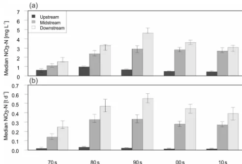
Figure 3.Flow-normalized median NO3–N concentrations(a)and NO3–N loads(b)for each decade of the time series and the three stations. Whiskers refer to the 5th and 95th percentiles of the WRTDS estimations.
during high-flow conditions, and vice versa: especially dur-ing HFSs, the median downstream contribution was less than 10 %, while during low-flow periods, the downstream contri-bution accounted for up to 33 % (summer).
The flow-normalized NO3–N concentrations in each
sub-catchment showed strong differences in their overall levels and temporal patterns over the four decades (Fig. 3a; see also Figs. 2 and 6 for details). The lowest decadal concen-tration changes and the earliest decrease in concenconcen-trations were found in the pristine catchment. Median upstream con-centrations were highest in the 80s (1987), with a reduction of the concentrations to about one-half in the latter decades. Over the entire period, the median upstream concentrations were smaller than 1 mg L−1, so that the described changes are small compared to the NO3–N dynamics of the more
downstream stations. High changes over time were observed in the two downstream stations with a tripling of concentra-tions between the 1970s and 1990s, when maximum concen-trations were reached. While median concenconcen-trations down-stream decreased slightly after this peak (1995/1996), the ones at the midstream station (peak: 1998) stayed constantly high. At the end of the observation period, at the outlet (downstream), the median annual concentrations did not de-crease below 3 mg L−1of NO3–N, a level that was exceeded
after the 1970s. The differences in NO3–N concentrations
between the pristine upstream and the downstream station evolved from an increase by a factor of 3 in the 1970s to a factor of 7 after the 1980s.
Calculated loads (Fig. 3b) also showed a drastic change between the beginning and the end of the time series. The daily upstream load contribution was below 10 % of the to-tal annual export at the downstream station in all decades and then the estimates decreased from 9 % (1970s) to 4 % (2010s). The median daily load between the 1970s and 1990s
tripled at the midstream station (0.1 to 0.3 t d−1) and more than doubled downstream (0.2 to 0.5 t d−1). In the 1990s, the
Holtemme River exported on average more than 0.5 t d−1of
NO3–N, which, related to the agricultural area in the
catch-ment, translates into more than 3.1 kg N km−2d−1 (maxi-mum 13.4 kg N ha−1a−1in 1995).
3.3 Input–output balance: N budget
We jointly evaluated the estimated N inputs and the exported NO3–N loads to enable an input–output balance. This
com-parison on the one hand allowed for an estimation of the catchment’s retention potential and on the other hand enabled us to estimate future exportable loads.
The load stemming from the most upstream, pristine catchment accounted for less than 10 % of the exported river-ine load at the outlet. To focus on the anthropogenic im-pacts, the data from the upstream station are not discussed on its own in the following. At the midstream station, a to-tal sum of input of 16 441 t compared to 4109 t of exported NO3–N for the overlapping time period of input and output
was analyzed (1970–2011). The midstream subcatchment re-ceived 73 % (Table 3) more N mass than it exported at the same time. Note that the exported N is not necessarily the N applied in the same period due to the temporal offset, as is discussed later in detail. With the assumption that 43 % (agricultural N input of subcatchment N input) of the diffuse input resulted from agriculture, the subcatchment exported 616 kg N ha−1(537–719 kg N ha−1) from agricultural areas. The cumulated N input from the entire catchment (measured downstream) from 1976 to 2015 (overlapping time of in-put and outin-put) was 53 437 t, while the riverine export in the same time frame was only 12 % (6 kg N ha−1a−1; 11 %–
14 %), implying an agricultural export of 370 kg N ha−1 (325–415 kg N ha−1; Fig. 4). This mass discrepancy between input and output translates into a retention rate in the entire Holtemme catchment of 88 % (86 %–89 %). In relation to the entire subcatchment area (not only agricultural land use), the annual retention rate of NO3–N was around 28 kg N ha−1a−1
(27–30 kg N ha−1a−1) in the midstream subcatchment and 59 kg N ha−1a−1 (59–59 kg N ha−1a−1) in the flatter and more intensively cultivated downstream subcatchment.
3.4 Effective TTs of N
We approximated the effective TTs for all seasonal NO3–N
Table 2.Descriptive statistics on discharge at the three observation points; LFS – low-flow season (June–November), HFS – high-flow season (December–May).
Upstream Midstream Downstream
[image:10.612.89.507.211.281.2]Median discharge (m3s−1) 0.23 0.9 1.1 Mean specific discharge (mm a−1) 768 411 178 LFS subcatchment contribution (%) 17 53 30 HFS subcatchment contribution (%) 21 69 10
Table 3.Nitrogen retention potentials derived for the midstream and downstream subcatchment based on flow-normalized fluxes. Numbers in brackets refer to the 5th and 95th percentiles of the WRTDS flux estimation.
Midstream Downstream
Retention cumulative (%) 75 (71–78) (Up-+midstream) 88 (86–89) (Up-+mid-+downstream) Retention subcatchment (%) 73 (68–76) 94 (94–95)
Retention per year (N kg a−1) 251 589 (235 778–263 833) 917 823 (968 085–979 679) Retention per area (N kg a−1ha−1) 28.43 (26.64–29.81) 58.82 (58.60–59.30)
and seasons can be observed, best represented by the mode of the distributions (peak TTs). The average deviation between the best- and worst-case estimation of the fitted TTDs from their respective average value was only 4 % with respect to the mode of the distributions (Table 4).
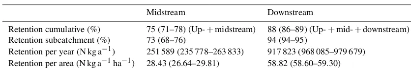
The TTDs for all seasons taken together showed longer TTs for the midstream in comparison to the downstream sta-tion. The comparison of the TTD modes for the different seasons at the midstream station showed distinctly differ-ing peak TTs between 11 years (sprdiffer-ing) and 22 years (fall), which represented a doubling of the peak TT. The fastest times appeared in the HFSs while modes of the TTDs ap-peared longer in the LFSs. Note that the shape factorσof the effective TTs also changed systematically: the HFS spring exhibited a higher shape factor than those of the other sea-sons. This refers to a change in the coefficient of variation of the distributions at the midstream station from 0.6 in spring to 0.2 in fall.
The modes of the fitted distributions for the downstream station for each season were shorter than the ones at the mid-stream station. The mode of the TTs ranged between 7 years (spring) and 15 years (winter, fall). The shape factors of the fitted TTDs ranged between 0.8 (spring) and 0.3 (sum-mer) for the downstream station. In summary, HFS spring in both subcatchments had shorter TTDs than the other seasons and the midstream subcatchment showed longer TTDs than downstream.
3.5 Seasonal NO3–N concentrations andC–Q relationships over time
As described above, the Holtemme catchment showed a pro-nounced seasonality in discharge conditions, producing the HFS in December–May (winter+spring) and the LFS in June–November (summer+fall). Therefore, changes in the
seasonal concentrations of NO3–N also reflect in the annual C–Qrelationship. Analyzing the changing seasonal dynam-ics therefore provide a deeper insight into N trajectories in the Holtemme catchment.
In the pristine upstream catchment, no temporal changes in the seasonal differences of riverine NO3–N concentrations
could be found (Fig. 6a). Also theC–Qrelationship (Fig. 6d) showed a steady pattern (moderate accretion), with the high-est concentrations in the HFSs, i.e., winter and spring. The ratio of CVC/CVQ indicates a chemostatic export regime and changed only marginally (amplitude of 0.2) over time.
At the midstream station (Fig. 6b), the early 1970s showed an export pattern with highest concentration during HFSs similar to the upstream catchment, but with a general in-crease in concentrations from 1970 to 1995. During the 1980s, the increase in concentrations in the HFS was faster than in the LFS, which changed the C–Q pattern to a strongly positive one (bmax=0.42, 1987; red to orange
sym-bols in Fig. 6e). This development was characterized by a tripling of intra-annual amplitudes (Cspring–Cfall) of up to
2.4 mg L−1 (1987). With a lag of around 10 years, in the
1990s the LFSs also exhibit a strong increase in concen-trations (Cmax=3.1 mg L−1, 1998, Fig. 6b). The midstream
concentration time series shows bimodality. TheC–Q rela-tionships (Fig. 6e) evolved from an intensifying accretion pattern in the 1970s and 1980s (red to orange symbols in Fig. 6e) to a constant pattern betweenCandQin the 1990s and afterwards (yellow symbols). The CVC/CVQincreased during the 1970s and strongly decreased afterwards by 0.4 between 1984 and 1995, showing a trajectory starting from a more chemostatic to a chemodynamic and then back to a chemostatic export regime.
Figure 4. Cumulative annual diffuse N inputs to the catchment and measured cumulative NO3–N exported load over time for mid-stream(a)and downstream(b)stations. Shaded grey confidence bands refer to the 5th and 95th percentile of the WRTDS flux estimation.
Table 4.Best-fit parameters of the log-normal TTDs for the N input and output responses. Parameters in brackets are derived by using the 5th and 95th percentiles of the bootstrapped flow-normalized concentration estimates.
Parameter All seasons Winter Spring Summer Fall
Midstream µ 3.0 (3.0–3.1) 3.0 (3.0–3.1) 2.7 (2.7–2.7) 3.0 (3.0–3.1) 3.1 (3.1–3.2) σ 0.3 (0.3–0.4) 0.3 (0.3–0.4) 0.6 (0.6–0.6) 0.3 (0.3–0.4) 0.2 (0.1–0.3) Mode (years) 18.5 (16.7–20.5) 17.8 (16.0–20) 11.1 (10.3–10.3) 18.9 (17.1–20.8) 21.9 (20.8–23.9) R2 0.93 (0.91–0.91) 0.88 (0.83–0.86) 0.81 (0.72–0.80) 0.91 (0.90–0.90) 0.87 (0.86–0.86)
Downstream µ 2.8 (2.8–2.9) 3.0 (3.0–3.0) 2.6 (2.7–2.7) 2.7 (2.7–2.7) 2.9 (2.9–2.9) σ 0.6 (0.5–0.6) 0.5 (0.5–0.5) 0.8 (0.7–0.8) 0.3 (0.2–0.3) 0.5 (0.5–0.5) Mode (years) 12.4 (12.1.–13.1) 15.1 (14.7–16.4) 7.4 (7.9–8.3) 13.8 (13.6–14.2) 14.7 (14.1–14.9) R2 0.94 (0.89–0.92) 0.92 (0.82–0.92) 0.84 (0.83–0.92) 0.90 (0.84–0.88) 0.81 (0.72–0.77)
at the midstream station. As seen at the midstream station, the N concentrations during the LFSs peaked with a delay compared to those of the HFSs. The resulting intra-annual amplitude showed a maximum of 2.4 mg L−1 in the 1980s (1983–1984), with strongly positive C–Qpatterns (bmax=
0.4, 1985; red symbols in Fig. 6f). In contrast to the bimodal concentration trends in the mid- and downstream HFSs, the LFSs downstream showed an unimodal pattern peak-ing around 1995–1996 with concentrations above 6 mg L−1 NO3–N (Cmax=6.9 mg L−1). In the 1990s, the
concentra-tions in the LFSs were higher than those noticed in the HFSs, causing a switch to a dilutionC–Qpattern (orange symbols in Fig. 6f). Due to the strong decline of LFS concentrations after 1995 (Fig. 6c), the dilution pattern evolved to a con-stantC–Qpattern (yellow symbols in Fig. 6f) from the 2000s onward. After an initial phase with chemostatic conditions (1970s), the CVC/CVQstrongly increased to a chemody-namic export regime in the 1980s (max. CVC/CVQ=0.8, 1984). Later on CVC/CVQdeclined by 0.8 between 1984 and 2001 (min. CVC/CVQ=0.03), which indicates theC–
Qtrajectory is coming back to a chemostatic export nitrate regime.
4 Discussion
4.1 Catchment-scale N budgeting
Based on the calculated budgets of N inputs and riverine N outputs for the three subcatchments within the Holtemme catchment, we discuss here differences between the sub-catchments and potential main reasons for the missing part in the N budget: (1) permanent N removal by denitrification or (2) the buildup of N legacies.
[image:11.612.57.540.320.440.2]Figure 5.Seasonal variations in the fitted log-normal distributions of effective travel times between nitrogen input and output responses for midstream(a)and downstream(b)stations.
The total input over the whole catchment area was quan-tified as more than 53 000 t N (1976–2015) and, compared to the respective output over the same time period, yielded ex-port rates of 25 % (22 %–29 %) at the midstream and 12 % (11 %–14 %) at the downstream station (Table 3), respec-tively. There can be several reasons for the difference in ex-port rates between the two subcatchments. The most likely ones are due to differences in discharge, topography and den-itrification capacity among the subcatchments, which are dis-cussed in the following.
Load export of N from agricultural catchments is assumed to be mainly discharge-controlled (Basu et al., 2010). Many solutes show a lower variance in concentrations compared to the variance in streamflow, which makes the flow vari-ability a strong surrogate for load varivari-ability (Jawitz and Mitchell, 2011). This can also be seen in the Holtemme catchment, which evolved over time to a more chemostatic export regime with high N loads (Fig. 6b). The highest N export and lowest retention were observed in the midstream subcatchment, where the overall highest discharge contribu-tion can be found.
Besides discharge quantity, we argue that the midstream subcatchment favors a more effective export of NO3–N. The
higher percentage of artificial drainage by tiles and ditches (59 % vs. 21 %; Sect. S1.1) as well as the steeper terrain slopes (3.2◦ vs. 1.9◦) in the nonforested area of the mid-stream catchment promotes rapid, shallow subsurface flows. These flow paths can more directly connect agricultural N sources with the stream and in turn cause elevated instream NO3–N concentrations (Yang et al., 2018a). In addition, the
steeper surface topography suggests a deeper vertical infil-tration (Jasechko et al., 2016) and therefore a wider range of flow paths of different ages than those observed in the flatter terrain areas, and vice versa: fewer drainage installations, a
flatter terrain and thus in general shallower flow paths may decrease the N export efficiency (increase the retention) po-tential downstream.
The only process able to permanently remove N input from the catchment is denitrification in soils, aquifers (Seitzinger et al., 2006; Hofstra and Bouwman, 2005), and at the stream-aquifer interface such as in the riparian (Vidon and Hill, 2004; Trauth et al., 2018) and hyporheic zones (Vieweg et al., 2016). As the riverine exports are signals of the catchment or subcatchment processes, integrated in time and space, sepa-rating a buildup of an N legacy from a permanent removal via denitrification is difficult. A clear separation of these two key processes, however, would be important for decision makers as both have different implications for management strate-gies and different future impacts on water quality. Even if groundwater quality measurements that indicate denitrifica-tion were available, using this type of local informadenitrifica-tion for an effective catchment-scale estimation of N removal via deni-trification would be challenging (Green et al., 2016; Otero et al., 2009; Refsgaard et al., 2014). Therefore, we discuss the denitrification potential in the soils and aquifers of the Holtemme catchment based on a local isotope study and a literature review of studies in similar settings. A strong ar-gument against a dominant role of denitrification is provided by Müller et al. (2018) for the study area. On the basis of a monitoring of nitrate isotopic compositions in the Holtemme River and in tributaries, Müller et al. (2018) stated that den-itrification played no or only a minor role in the catchment. However, we still see the need to carefully check the poten-tial of denitrification to explain the input–output imbalance considering other studies.
Figure 6.Annual N input (referring to the whole catchment, secondyaxis) to the catchment and measured median NO3–N concentrations in the stream (firstyaxis) over time at three different locations: upstream(a, d), midstream(b, e), downstream(c, f). Lower panels show plots of slopebvs. CVC/CVQfor NO3–N for the three subcatchments following the classification scheme provided in Musolff et al. (2015). The xaxis gives the coefficient of variation of concentrations (C) relative to the coefficient of variation of discharge (Q). Theyaxis gives the slope b of the linear ln(C)–ln(Q) relationship. Colors indicate the temporal evolution from 1970 to 2015 along a gradient from red to yellow.
would need a rate of 74.9 kg N ha−1a−1. Considering the
de-rived TTs, denitrification of the convolved input would need a slightly lower rate (66.7 kg N ha−1a−1, 1976–2015). Deni-trification rates in soils for Germany (NLfB, 2005) have been reported to range between 13.5 and 250 kg N ha−1a−1, with rates larger than 50 kg N ha−1a−1may be found in carbon-rich and waterlogged soils in the riparian zones near rivers and in areas with fens and bogs (Kunkel et al., 2008). As wa-ter bodies and wetlands make up only 1 % of the catchment’s land use (Fig. 1; EEA, 2012), and consequently the extent of waterlogged soils is negligible, denitrification rates larger than 50 kg N ha−1a−1are highly unlikely. In a global study, Seitzinger et al. (2006) assumed a rate of 14 kg N ha−1a−1as denitrification for agricultural soils. With this rate only 19 % of the retained (88 %) study catchment’s N input can be deni-trified. On the basis of a simulation with the modeling frame-work GROWA-WEKU-MEPhos, Kuhr et al. (2014) estimate very low to low denitrification rates, of 9–13 kg N ha−1a−1,
for the soils of the Holtemme catchment. Based on the above discussion we find for our study catchment, the denitrifica-tion in the soils, including the riparian zone, may partly ex-plain the retention of NO3–N, but there is unlikely to be a
single explanation for the observed imbalance between input and output.
Regarding the potential for denitrification in groundwater, the literature provides denitrification rate constants of a first-order decay process between 0.01 and 0.56 a−1(van Meter et al., 2017b; van der Velde et al., 2010; Wendland et al., 2005). We derived the denitrification constant by distributing the input according to the fitted log-normal distribution of TTs, assuming a first-order decay along the flow paths (Kuhr et al., 2014; Rode et al., 2009; van der Velde, 2010). The denitrification of the 88 % of input mass would require a rate constant of 0.14 a−1. This constant is in the range of values
al. (2018) provide strong evidence that denitrification in the groundwater of the Holtemme catchment is not a dominant retention process. More specifically, Hannappel et al. (2018) assess denitrification in over 500 wells in the federal state of Saxony-Anhalt for nitrate, oxygen, iron concentrations and redox potential and connect the results to the hydrogeologi-cal units. Within the hard rock aquifers that are present in our study area, only 0 %–16 % of the wells showed signs of den-itrification. Taking together the local evidence from the ni-trate isotopic composition (Müller et al., 2018), the regional evidence from groundwater quality (Hannappel et al., 2018), and the rates provided in literature for soils and groundwa-ter, we argue that the role of denitrification in groundwater is unlikely to explain the observed imbalance between N input and output.
Lastly, assimilatory NO3uptake in the stream may be a
po-tential contributor to the difference between input and output. But even with maximal NO3uptake rates as reported by
Mul-holland et al. (2004; 0.14 g N m−2d−1) or Rode et al. (2016; max. 0.27 g N m−2d−1, estimated for a catchment adjacent to the Holtemme), the annual assimilatory uptake in the river would be a minor removal process, estimated to contribute only 3 % of the 88 % discrepancy between input and output. According to the rates reported by Mulholland et al. (2008; max. 0.24 g N m−2d−1), the Holtemme River would need an area 45 times larger to be able to denitrify the retained N. Therefore denitrification in the stream can be excluded as a dominant removal process.
In summary, the precise differentiation between the accu-mulation of an N legacy and removal by denitrification can-not be fully resolved on the basis of the available data. Also a mix of both may account for the missing 88 % (86 %–89 %, downstream) or 75 % (71 %–78 %, midstream) in the N out-put. Input–output assessments with time series from differ-ent catchmdiffer-ents, as presdiffer-ented in van Meter and Basu (2017), covering a larger variety of catchment characteristics, hold promise for an improved understanding of the controlling pa-rameters and dominant retention processes.
The fact that current NO3 concentration levels in the
Holtemme River still show no clear sign of a significant de-crease calls for a continuation of the NO3concentration
mon-itoring, best extended by additional monitoring in soils and groundwater. Despite strong reductions in agricultural N in-put since the 1990s, the annual N surplus (e.g., 818 t a−1, 2015) is still much higher than the highest measured export (loadmax=216 t a−1, 1995) from the catchment. Hence, the
difference between input and output is still high with a mean factor of 6 during the past 10 years (mean factor of 7 with the shifted input according to 12 years of TT). Consequently, ei-ther the legacy of N in the catchment keeps growing instead of getting depleted or the system relies on a potentially lim-ited denitrification capacity. Denitrification may irreversibly consume electron donors like pyrite for autolithotrophic den-itrification or organic carbon for heterotrophic denden-itrification (Rivett et al., 2008).
Based on the analyses and literature research, there is ev-idence but no proof of the fate of missing N, although a di-rected water quality management would need a clearer dif-ferentiation between N mass that is stored or denitrified. However, neither tolerating the growing buildup of legacies nor relying on finite denitrification represents sustainable and adapted agricultural management practices. Hence, fu-ture years will also face increased NO3–N concentrations and
loads exported from the Holtemme catchment.
4.2 Linking effective TTs, concentrations andC–Q trajectories with N legacies
Based on our data-driven analyses, we propose the following conceptual model (Fig. 7) for N export from the Holtemme catchment, which is able to plausibly connect and synthesize the available data and findings on TTs, concentration trajec-tories andC–Qrelationships and allows for a discussion on the type of N legacy.
Over the course of a year, different subsurface flow paths are active, which connect different subsurface N source zones with different source strength (in terms of concen-tration and flux) to streams. These flow paths transfer wa-ter and NO3–N to streams, predominantly from shallower
parts of the aquifer when water tables are high during HFSs and exclusively from deeper groundwater during low flows in LFSs (Rozemeijer and Broers, 2007; Dupas et al., 2016; Musolff et al., 2016). This conceptual model allows us to explain the observed intra-annual concentration patterns and the distinct clustering of TTs into low-flow and high-flow conditions. Furthermore, it can explain the mobilization of nutrients from spatially distributed NO3–N sources by
tem-porally varying flow-generating zones (Basu et al., 2010). Spatial heterogeneity of solute source zones can be a re-sult of downward migration of the dominant NO3–N storage
zone in the vertical soil–groundwater profile (Dupas et al., 2016). Moreover, a systematic increase in the water age with depths would, if denitrification in groundwater takes place uniformly, lead to a vertical concentration decrease. Based on the stable hydroclimatic conditions without changes in land use, topography or the river network during the obser-vation period, long-term changes in flow paths in the catch-ment are unlikely. Assuming that flow contributions from the same depths do not change between the years, the observed decadal changes in the seasonal concentrations cannot be ex-plained by a stronger imprint of denitrification with increas-ing water age. Under such conditions one would expect a more steady seasonality in concentrations andC–Qpatterns over time with NO3–N concentrations that are always
Figure 7.Conceptual model of nitrogen legacy and exports from the midstream and the downstream catchments. The four stacked boxes refer to the dominant source layer of nitrate that is activated with changing water level and catchment wetness during low-flow seasons fall (red) and autumn (orange) as well as high-flow seasons winter (blue) and spring (green). Numbers in the boxes refer to peak travel times of each season. The percentages refer to the N imbalance between input and output explainable by travel times (hydrological legacy). Background map created from ATKIS data.
input is one of the most likely plausible explanations for our observations with regard to N budgets, concentrations and C–Qtrajectories.
The faster TTs observed at the midstream station during HFSs are assumed to be dominated by discharge from shal-low (near-surface) source zones. This zone is responsible for the fast response of instream NO3–N concentrations to the
increasing N inputs (1970s to mid-1980s). This faster lateral transfer, especially in spring (shortest TT), may be also en-hanced by the presence of artificial drainage structures such as tiles and ditches. In line with the longer TTs during the LFSs, low-flow NO3–N concentrations were less impacted
in the 1970s to mid-1980s as deeper parts of the aquifer were still less affected by anthropogenic inputs. With time and a downward migration of the high NO3–N inputs before 1990,
those deeper layers and thus longer flow paths also delivered increased concentrations to the stream (1990s). In parallel with the increasing low-flow concentrations (in the 1990s), the spring concentrations of NO3decreased, caused by a
de-pletion of the shallower NO3–N stocks (see also Dupas et
al., 2016; Thomas and Abbott, 2018). This depletion of the stocks was a consequence of drastically reduced N input af-ter the German reunification in 1989. This conceptual model of N trajectories is supported by the changing C–Q rela-tionship over time. The seasonal cycle started with increas-ing NO3–N maxima during high flows and minima during
low flows, since shallow source zones were getting loaded with NO3first. Consequently, the accretion pattern was
in-tensified in the first decades, accompanied by an increase in CVC/CVQ. The resulting positiveC–Q relationship on a
seasonal basis was found in many agricultural catchments worldwide (e.g., Aubert et al., 2013; Martin et al., 2004; Mel-lander et al., 2014; Rodríguez-Blanco et al., 2015; Musolff et al., 2015). However, after several years of deeper migra-tion of the N input, the catchment started to exhibit a chemo-static NO3export regime (after the 1990s), which was
man-ifested in the decreasing CVC/CVQratio. This stationarity could have been caused by a vertical equilibration of NO3–N
concentrations in all seasonally activated depth zones of the soils and aquifers after a more stable long-term N input after 1995. According to the 50th percentile of the derived TT, af-ter 20 years only 50 % of the input had been released at the midstream station. Therefore without any strong changes in input, the chemostatic conditions caused by the uniform, ver-tical NO3–N contamination will remain. At the same time,
this chemostatic export regime supports the hypothesis of an accumulated N legacy rather than denitrification as the dom-inant reason for the imbalance between input and output.
At the downstream station, the riverine NO3
concentra-tions during high flows were dominated by inputs from the midstream subcatchment, which explains the similarity with the midstream bimodality in concentrations as well as the comparable TTs. The reason for these dominating midstream flows is the strong precipitation gradient resulting in a runoff gradient on the leeward side of the mountains. During low flows, the downstream subcatchment can contribute much more to discharge and therefore to the overall N export. Dur-ing the LFSs, we observed higher NO3–N concentrations
sub-catchment supports higher water levels and thus faster TTs during the low flows. Greater prevalence of young stream-flow in flatter lowland terrain was also described by Jasechko et al. (2016). But besides the earlier peak time during low flows, the concentration was found to be much higher than at the midstream station. To cause such high intra-annual con-centration changes, the downstream NO3–N load
contribu-tion, e.g., during the concentration peak of 1995–1996, had to be high: the summer season export was 46 t, which is more than twice the median contribution during summer (22 t). A more effective export from the downstream catchment hap-pened mainly during LFSs, which is also supported by the narrower TTD (small shape factor σ) in the summer and fall (Fig. 5b). The difference between the 75th and 25th per-centiles (5 years) was also the smallest of all seasons in the summer at the downstream station. This could be one reason for the high concentrations in comparison to the midstream catchment and during the HFSs.
In contrast to the midstream catchment, theC–Q trajec-tory in the downstream catchment temporarily switched from an enrichment pattern, dominated by the high concentration during high flows from the midstream catchment to a dilution pattern and a chemodynamic regime, when the high concen-trations in the LFS from the downstream subcatchment domi-nated. Although the low-flow concentrations were slowly de-creasing in the 2000s and 2010s, the downstream catchment also finally evolved to a chemostatic NO3export regime, as
was noticed at the midstream station (Fig. 6f).
Our findings support the evolution from chemodynamic to chemostatic behavior in managed catchments, but also em-phasize that changing inputs of N into the catchment can lead to fast-changing export regimes even in relatively slowly reacting systems. Our findings expand on previous knowl-edge (Basu et al., 2010; Dupas et al., 2016) as we could show systematic interannual C–Qchanges that are in line with a changing input and a systematic seasonal differenti-ation of TTs. Although our study showed chemostatic be-havior towards the end of the observation period (mid- and downstream; Fig. 6e–f), this export regime is not necessar-ily stable as it depends on a continuous replenishment of the legacy store. Changes in the N input translate to an in-crease in spatial heterogeneity in NO3–N concentrations in
soil water and groundwater with contrasting water ages. The seasonally changing contribution of different water ages thus results in more chemodynamic NO3export regimes. As
de-scribed in Musolff et al. (2017), both export regimes and pat-terns are therefore controlled by the interrelation of TT and source concentrations. We argue that a hydrological legacy of NO3in the catchment has been established that resulted in
the pseudo-chemostatic export behavior we observe nowa-days. This supports the notion that a biogeochemical legacy corresponding to the buildup of organic N in the root zones of the soil (van Meter et al., 2016) is less probable. If we assume that all of the 88 % of the N input is accumulating in the soils, we cannot explain the observed shorter-term
in-terannual concentration changes and trajectory in theC–Q relationships. We would rather expect a stronger and even growing dampening of the N input to the subsurface with the buildup of a biogeochemical legacy in the form of organic N. However, we cannot fully exclude the accumulation of a protected pool of soil organic matter with very slow mineral-ization rates as described in van Meter et al. (2017). Our con-ceptual model assigns the missing N to the long TTs of NO3–
N in soil water and groundwater and in turn to a pronounced hydrological legacy. In the midstream subcatchment, the esti-mated TTD explains 40 % of the retained NO3–N, comparing
the convolution of TTD with the N input time series to the ac-tual riverine export. The remaining 60 % cannot be fully ex-plained at the moment and may be assigned to a permanent removal by denitrification (see discussion above), to a fixa-tion due to the biogeochemical legacy or to more complex (e.g., longer tailed) TTDs, which are not well represented by our assumed log-normal distribution. In the downstream sub-catchment, our approach explains 29 % of the observed ex-port. This could in principle be caused by the same processes as described for the midstream subcatchment. A hydrologi-cal legacy store in deeper zones without significant discharge contribution is also possible (Fig. 7). That mass of N is either bypassing the downstream monitoring station (note that the downstream station is still 3 km upstream of the Holtemme catchment outlet) or is affected by a strong time delay and dampening not captured by our approach. Consequently, fu-ture changes in N inputs will also change the fufu-ture export patterns and regimes, since this would shift the homogeneous NO3–N distributions in vertical soil and groundwater profiles
back to more heterogeneous ones.
5 Conclusion
In the present study we used a unique time series of riverine N concentrations over the last four decades from a mesoscale German catchment as well as estimated N input to discuss the linkage between the two on annual and intra-annual timescales. From the input–output assessment, the buildup of a potential N legacy was quantified, effective TTs of ni-trate were estimated and the temporal evolution to chemo-static NO3–N export was investigated. This study provides
four major findings that can be generalized and transferred to other catchments of similar hydroclimatic and landscape settings as well.
still on the way to the stream, may have strong effects on future water quality and long-term implications for river wa-ter quality management. With a median export rate of 162 t N a−1 (1976–2016, downstream station, 6 kg N ha−1a−1), a depletion of this legacy (<46 000 t N) via baseflow would maintain elevated riverine concentrations for the next few decades. Although N surplus strongly decreased after the 1980s, during the past 10 years there was still an imbalance between agricultural input and riverine export by a mean fac-tor of 5 (assuming the temporal offset of peak TTs between input and output of 12 years). This is a nonsustainable con-dition, regardless of whether the retained nitrate is stored or denitrified. Export rates as well as retention capacity derived for this catchment were found to be comparable to findings of other studies in Europe (Worrall et al., 2015; Dupas et al., 2015) and North America (van Meter et al., 2016).
Second, we derived peak time lags between N input and riverine export between 7 and 22 years with systematic dif-ferences among the different seasons. Catchment managers should be aware of these long time frames when imple-menting measures and when evaluating them. This study ex-plains the seasonally differing lag times and temporal con-centration evolutions with the vertical migration of the ni-trate and their changing contribution to discharge by season-ally changing aquifer connection. Hence, interannual con-centration changes are not dominantly controlled by inter-annually changing discharge conditions, but rather by the seasonally changing activation of subsurface flows with dif-fering ages and thus difdif-fering N loads. As a consequence of this activation-dependent load contribution, an effective, adapted monitoring needs to cover, different discharge condi-tions when measures shall be assessed for their effectiveness. In the light of comparable findings of long time lags (van Me-ter and Basu, 2017; Howden, 2011), there is a general need for sufficient monitoring length and appropriate methods for data evaluation like the seasonal statistics of time series.
Third, in contrast to a more monotonic change from a chemodynamic to a chemostatic nitrate export regime that was observed previously (Dupas et al., 2016; Basu et al., 2010), this study found a systematic change in the nitrate export regime from accretion over dilution to chemostatic behavior. Here, we can make use of the unique situation in East German catchments where the collapse of agriculture in the early 1990s provided a large-scale “experiment” with abruptly reduced N inputs. While previous studies could not distinguish between biogeochemical and hydrological legacy to cause chemostatic export behavior, our findings provide support for a hydrological legacy in the study catchment. The systematic interannual changes inC–Qrelationships of NO3–N were explained by the changes in the N input in
com-bination with the seasonally changing effective TTs of N. The observed export regime and pattern of NO3–N suggest a
dominance of a hydrological N legacy over the biogeochem-ical N legacy in the upper soils. In turn, observed trajectories in export regimes of other catchments may be an indicator of
their state of homogenization and can be helpful to classify results and predict future concentrations.
Fourth, although we observed long TTs, significant input changes also created strong interannual changes in the export regime. The chemostatic behavior is therefore not necessar-ily a persistent endpoint of intense agricultural land use, but depends on steady replenishment of the N store. Therefore, the export behavior can also be termed pseudo-chemostatic and may further evolve in the future (Musolff et al., 2015) under the assumptions of a changing N input. Depending on the legacy size, a significant reduction or increase in N input can cause an evolution back to more chemodynamic regimes with dilution or enrichment patterns. Simultaneously, input changes affect the homogenized vertical nitrate profile, re-sulting in larger intra-annual concentration differences and consequently chemodynamic behavior. Hence, chemostatic behavior and homogenization may be characteristics of man-aged catchments, but only under constant N input.
Recommendations for a sustainable management of N pol-lution in the studied Holtemme catchment, also transferable to comparable catchments, focus on the two aspects: deplet-ing past inputs and reducdeplet-ing future ones.
Our findings could not prove a significant loss of NO3–N
by denitrification. To deal with the past inputs and to focus on the depletion of the N legacy, end-of-pipe measures such as hedgerows around agricultural fields (Thomas and Abbott, 2018), riparian buffers or constructed wetlands may initiate N removal by denitrification (Messer et al., 2012).
We could show that there is still an imbalance of agricul-tural N input and riverine export by a mean factor of 5. A reduced N input due to better management of fertilizer and the prevention of N losses from the root zone at the present time is indispensable to enable depletion instead of a further buildup or stabilization of the legacy.