Canadian Labour Market
and Skills Researcher
Network
Working Paper No. 94
CLSRN is funded by the Social Sciences and Humanities Research Council of Canada (SSHRC) under its Strategic Knowledge Clusters Program. Research activities of CLSRN are carried out
with support of Human Resources and Skills Development Canada (HRSDC). All opinions are those of the authors and do not reflect the views of HRSDC or the SSHRC.
Persistence and Academic Success in University
Martin D. Dooley McMaster University A. Abigail Payne McMaster University A. Leslie Robb McMaster University February 2012
Persistence and Academic Success in University
Martin D. Dooley, A. Abigail Payne, A. Leslie Robb
Department of Economics
McMaster University
Abstract
We use a unique set of linked administrative data sets to explore the determinants of persistence and academic success in university. The explanatory power of high school grades greatly dominates that of other variables such as university program, gender, and neighbourhood and high school characteristics. Indeed, high school and neighbourhood characteristics, such as average standardized test scores for a high school or average neighbourhood income, have weak links with success in university.
JEL Code: I23
Executive Summary
We address a series of questions concerning academic persistence and success among university students using administrative data that have been collected on
students in four Ontario universities and linked with information on the students’
individual characteristics (including high school performance), neighborhood, and high school. The students came directly from an Ontario high school and entered one of our four universities for full-time degree study in the fall of 1994 through 2006. The
measures of persistence are the cumulative grade average and credits completed at the end of Year 2, departures during the first two years, and degrees completed within six years. The following lessons can be inferred from our analyses.
First, the time trends reveal that the values of all four outcomes have generally been quite stable over time at each of our institutions. This stability over time in the levels of our measures of academic success in university is true of both the simple means of the variables and when we control statistically for a wide variety of individual, neighbourhood and school characteristics.
Second, academic performance in secondary school is strongly linked to all of our measures of university performance. These links are strong in the sense of both the magnitude and the precision of the estimated coefficients. Furthermore, the explanatory power of the high school grade average greatly dominates that of other variables such as university program, gender, neighbourhood average income, and average high school performance on Grade 9 EQAO tests. Understanding what lies behind the large estimated impact of high school grades is clearly important for understanding the determinants of university success. Many background factors
undoubtedly contribute to academic success in both high school and university including health, parental education and income, and the secondary schooling context. This policy concern highlights the importance of linking our current data sets to other data, such as from the Ministry of Education, that can shed light on the factors associated high school grades.
Third, the neighbourhood characteristics used in this study, including average income and others, have relatively weak links with our measures of persistence. In contrast, Dooley, Payne and Robb (2009) reported that students from low income neighbourhoods are 13 per cent less likely to apply to university than those in high income neighbourhoods (controlling for other factors including GPA) and that this gap in application rates over the last decade has remained relatively constant. Hence,
neighbourhood socio-economic background appears to play an important role in gaining access to university but a more minor role in academic success once a student has registered. We hasten to add, however, that numerous small differences can still have a large cumulative impact on the life of a young person. Furthermore, there is much variation in income and other socio-economic characteristics within neighbourhoods. Differences in individual family income may have substantially more success in
explaining university persistence than do differences in average income and education across neighbourhoods. Judged by our results to date, however, our four universities
appear to be institutions in which students from diverse non-academic backgrounds progress and succeed at similar rates and in similar proportions.
Fourth, our results point to the advantages of rich administrative data. Such data not only provide a very large sample size but also suffer much less than do survey data from response and selection bias. For example, one could do much additional research by examining additional outcome measures and conducting more specific analysis by program, academic level, gender, mother tongue, and type of high school. As indicated above, linking our current data with additional data sets will expand the research
1. Introduction
This paper addresses a series of questions concerning persistence and academic success among university students. What characterizes those students who have a high quality educational experience as measured by accumulated credits and cumulative grade averages? What differentiates those students who continue in the university at which they first register from those who leave within one or two years? What distinguishes those who complete a university degree, from those who fail to do so within a reasonable span of time? These questions have received substantially less attention in the literature than has the question of access to postsecondary education. We examine persistence and success using a rich administrative data set that links information on individual students at four Ontario universities with information on the high school performance of individual students, the high school that the student attended, and the neighbourhood in which the student grew up. These data sets provide many relevant variables, a large number of observations, and the actual measures (not self-reports) of such academic outcomes as grade averages and credits and degrees completed.
We find that the explanatory power of the high school grade point average (GPA) greatly dominates that of other variables such as university program, gender, and neighbourhood and high school characteristics. Indeed, high school and neighbourhood have weak links with success in university, regardless of whether we use specific measures, such as average test scores for a high school or average neighbourhood income, or models with fixed effects for high schools or neighbourhoods.
Section 2 contains a review of the literature. The data and variables are described in Section 3. The summary statistics are discussed in Section 4 and the multivariate analysis in Section 5. Section 6 provides a policy discussion and conclusion.
2
In a recent review, Mueller (2008b) confirms the overall paucity of Canadian studies of persistence in post-secondary education and highlights recent contributions in several areas. One such area is the sometimes complex pathways to degree completion. Using the Youth in Transition Survey (YITS), Finnie and Qiu (2008) found that only 52.1 per cent of university students complete a degree at their initial institution within five years, but completion rates rise to 73.1 per cent when one includes students who switched institutions or left school temporarily. Finnie and Qiu (2009) make the same point using system-wide administrative data for the Atlantic provinces.
A second area of recent research is the determinants of degree completion. Martinello (2008) found that parental education in the YITS did not correlate with completion of a first program of postsecondary education (PSE) but did correlate with completion of second program among those who switched. Bowlby and McMullen (2002) found greater persistence toward completion among YITS students who reported more parental income and scholarships. However, Johnson (2008) found little evidence in the YITS that higher tuition alters the probability of leaving university without a degree. Chemin (2009), using the YITS, reported that a 2001 increase in the value of student grants in Quebec increased PSE participation rates but not graduation rates relative to other provinces. Mueller (2008a) reports that finances may play a weak role in persistence, but the evidence is largely from surveys that ask students the reasons for dropping out.
Historically, PSE administrative data have primarily been used by individual institutions hoping to improve retention of their own students (Grayson and Grayson 2003). Recent uses of such data for research purposes are US-based study by Nora et al. (2005) and two Canadian papers (Finnie and Qui 2009 and Conrad and Morris 2010). None of the aforementioned studies, however, link university files with data on individual high school performance and both high school and neighbourhood characteristics. The current study provides a major step forward in this regard.
3 3. Data and Measures
3.1 University Administrative Data and Persistence Measures
Four Ontario universities provided student-level information. Two are of the medical/doctoral variety, one is comprehensive, and one is primarily undergraduate.1 The combined undergraduate enrolments at
these universities averaged 28% of the total at Ontario universities over our sample period. Our data set is limited to students who entered a full time university degree program directly from an Ontario high school in September.2 These student types comprise over 90% of all entering undergraduates students at
Ontario universities (Dooley, Payne and Robb, 2009). Two universities provided data for entering cohorts in September of 1994 through 2004. The entering dates were 1994 through 2005 for the third school and 1999 through 2006 for the fourth school.
We distinguish students by four academic programs upon entry: Arts, Science, Business and Engineering. Students in smaller entry programs were assigned to one of these four, e.g., students in Kinesiology were assigned to Science and those in Music to Arts. Table A-1 provides definitions and sample means of our variables and the first four rows indicate the distribution by entry program. Three-quarters of our students enter Arts or Sciences while Engineering or Business account for the remaining one-quarter.
The universities provided information on credits earned and grade averages for each student by academic term (fall, winter and summer). In this article, we measure these indicators on a twelve-month (September through August) basis because of coop students whom we cannot directly identify and who
1 These designations are taken from a well-known classification system for Canadian universities created by Maclean’s magazine.
2We also excluded a small number of other observations for reasons such as a missing variable. See Dooley, Payne and
4
are less likely than non-coop students to be enrolled in fall and winter terms and more likely to be enrolled in the summer term.
Panel A of Table A-1 reports the measures of academic persistence and success on which we will focus, the first of which is the cumulative grade average at the end of two years. Year one here means the twelve-month period following a September entry while year two means months 13 through 24 following that entry. Our multivariate analysis revealed similar relationships between the one-year and two-year cumulative grade averages and the characteristics of individual students, neighbourhoods and high schools. Hence, we focus on the two year results for grades and for the next two outcomes. See Dooley, Payne and Robb (2011) for details of how we transformed all university records to a 0-100 grading system. The sample mean is 72 based on a sample of 113,271.3
Our second persistence measure is credits completed after 2 years. We use a credit system under which 0.5 credits is given for a one-term course. The sample mean is 9.2. Our third measure of persistence is a measure of departure (non-continuation). We use the term “departure” rather than “dropout” because we do not know the destination of students who cease to register for courses in each of our four universities. Some departures are undoubtedly voluntary transfers or temporary absences as documented by Finnie and Qiu (2008).4 We count as a “departure during the first two years” any
student for whom we have no grade for courses in the fall, winter or summer of the third academic year from among those students for whom we have at least three years of data. Table A-1 indicates that the departure rate during the first two years is 13%.
Our final measure of persistence is degree completion. The degrees in our data are designed to take three, four or five years to complete on a full-time basis. However, many students take more than the standard number of full-time years due to coop terms, program switches, periods of part-time study, academic terms abroad, etc. Only 45% of the students in our sample complete any degree within four
3Our total number of observations is 128,166 but the most recent entry cohorts in our sample are observed for only one year. 4 Students who depart do have lower than average grades and cumulative credits completed than those who do not depart.
5
years and such students are disproportionately from Arts and Science programs and universities with fewer coop programs. A six year window is common in other studies of degree completion ( See, for example, Nory, Barlow and Crisp 2005) and that is the standard which we have adopted.5 Table
A-1 shows that the proportion of students completing a degree within six years is 80%. 3.2 Individual, Neighbourhood and High School Characteristics
Individual Characteristics. All Ontario students applying to Ontario universities submit a common form to the Ontario Universities Application Centre (OUAC).6 Panel B of Table A-1 provides definitions and sample means for the OUAC variables. Fifty-five per cent of our students are females, 85% have English as mother tongue, 93% are Canadian citizens, and 94% have a home residence within 50 kilometres of campus. The students’ mean age at registration is 18.5 years. OUAC also has grade data provided directly by the highs schools. We use the average grade in the student’s best six Grade 12/13 University level courses.7 Panel B of Table A-1 indicates that 17% of students have an average
of 90 to 100 and 27% have an average of less than 80.
Neighbourhood Characteristics. The postal code in the OUAC data allows us to link the residence of the student’s family at the time of application to the corresponding census neighbourhood data for Enumeration Areas (EA) in 1996 and Dissemination Areas (DA) in 2001 and 2006. The details of how we performed this linkage are available in Dooley, Payne and Robb (2011). Our key income measure is “average equivalent income” which is average neighbourhood income divided by the square
5 We have not used the distinction between a “General” degree and an “Honours” degree in our analysis. Many “General” degree programs take four full-time years just like an “Honours” degrees. Furthermore, some non-Honours programs, such as Engineering, make academic demands of the student that are at least as extensive as Honours degrees in other disciplines. 6 Mature Ontario applicants and non-Ontario applicants follow a different application procedure, are relatively small in number, and come from very heterogeneous academic backgrounds
7 Our data period witnessed a major change in the secondary school curriculum in 2003 that shortened the normal number of years of high school for university bound students from five to four. Our grade average is of six Grade 13 courses for students from pre-reform cohorts and six Grade 12 University (or U/M) level courses for students from post-reform cohorts. This also resulted in a “double cohort” that entered university in 2003. The average on the best 6 courses is the generally accepted admission average for Ontario universities though different universities may calculate it slightly differently (how are repeated attempts treated, for example).
6
root of the neighbourhood average number of persons per household.8 The principal income indicator
that we use in this paper is whether a student is from a low-, middle- or high-income neighbourhood. In order to assess this, we calculated the distribution of average equivalent income across all EAs and DAs in the province weighted by total population. As indicated in Panel C of Table A-1, 18% of the students from our four universities are from neighbourhoods in the bottom tercile (one-third) of this distribution, 31% are from the middle tercile and 50% from the top tercile. 9 These values reflect the fact that
university students come disproportionately from more affluent neighbourhoods. Table A-1 also describes five other neighbourhood measures that we use. Our students come from neighbourhoods in which, on average, 21% of the adults have a Bachelor’s Degree or more, 11% of the families are headed by a lone mother, 87% of persons have English for a mother tongue, 13% of persons have immigrated to Canada since 1981, and 7% of adults are unemployed.
High School Characteristics. We also have information on the characteristics of our students’ high schools from the Ontario Ministry of Education for the years 2000 through 2003 (our data are incomplete over other years). A key variable that we use to assess the academic quality of a high school is the proportion of the students taking the Grade 9 standardized Academic Math Assessment that received a “high score” (3 or 4).10 We ordered all high schools in the OUAC data by this measure and
determined the cutoffs for the bottom (61%) and top (71%) terciles.11 Panel D of Table A-1 shows that
22% of our students are from high schools in the bottom tercile of this frequency distribution, 32% are from schools in the middle tercile and 46% are from schools in the top tercile. As expected, students at our four universities come from high schools with above average performance on the Grade 9 Math
8
Standardizing households of different sizes by use of an ‘equivalence scale’ is now quite common. The square root scale is one of the simplest and most commonly employed.
9Mean average equivalent income over all sample years is $45,504 (2001 dollars). Different tercile cutoffs were calculated
for each entry year. See Dooley, Payne and Robb (2011) for details.
10The Grade 9 Math Assessmenttest is a province wide assessment of the math skills students are expected to have learned by Grade 9. Students who are working toward their Grade 9 academic and applied math credit take different versions of this test. These are commonly called EQAO (Education, Quality and Accountability Office) exams.
7
Assessment. Table A-1 also reveals that 8% of students in the persistence data set are from high schools for which these standardized math scores are missing.12 The average student in the persistence data set
attended a high school that is 34 kilometres from the nearest university and 24 kilometres from the nearest college. Seven per cent of students come from private high schools, 70% from English public schools, 0.1% from Francophone public schools, 22.5% from English Catholic schools, and 0.4% from Francophone Catholic schools. Sixteen percent are from rural high schools. Finally, we ranked all high schools in the province by enrolment. Twenty-four per cent 24% of our students are from high schools in the bottom tercile of this frequency distribution, 34% are from schools in the middle tercile and 44% are from schools in the top enrolment tercile. Our university students come from high schools that are larger than average.
Finally, Panel E of Table A-1 shows the distribution of students in our data by year of entry to university. Changes in this proportion over time reflects both changing cohort size, especially the “double cohort” (see Footnote 7 above), and the fact that different universities provided data for differing periods of time (see Section 3.1 above).
4. Summary Statistics
Table 1 compares the students from the four universities for which we have data (the Persistence Data) with all OUAC applicants from Ontario High School students. For this comparison, we use data from 1999 through 2004 which are the years for which we have information from all four universities. Our four-university sample contains 20% of all OUAC applicants and 28% of all OUAC registrants in Ontario universities over the same time period. The students in our four universities, when compared to
12There is a large overlap between private schools and missing standardized math scores. Ninety-five per cent (95%) of private high schools have missing standardized math scores and 77% of the schools with missing standardized math scores are private.
8
all applicants or registrants, are slightly younger, have higher grades, and are more likely to have a mother tongue that is English and to be Canadian citizens. Generally, though, we believe that Table 1 indicates that the students from our four universities are reasonably similar to all students in Ontario universities.13
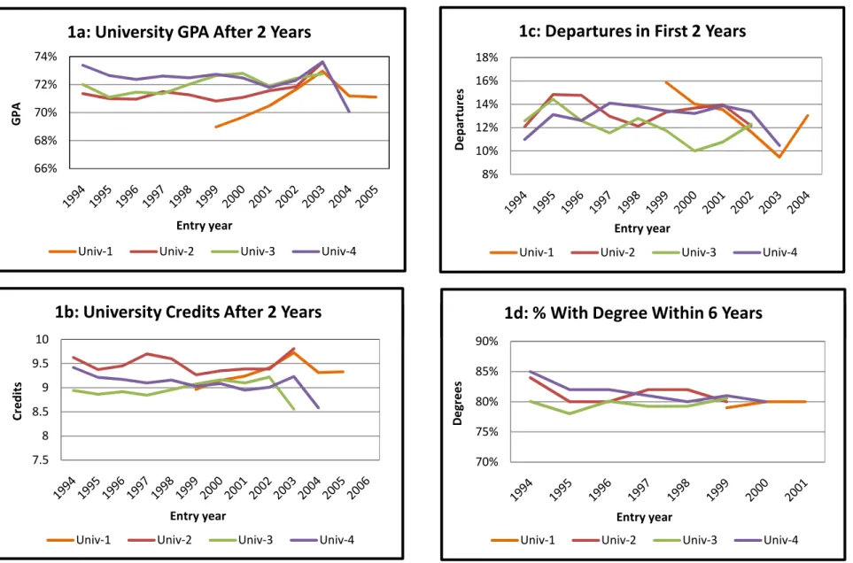
Figures 1a through 1d contain the time series plots for the four measures of academic progress described in Section 3.1 at each of our universities. We draw three basic conclusions from these figures. First, there are only minor differences among our four universities and the rank order changes over time. Second, these measures have generally been quite stable over time at each of our universities. There is no indication that rising tuition and other changes in the academic environment have led to lower (or higher) levels of success. Third, the figures do reveal some minor improvements in outcomes for the “double cohort” that entered in 2003. This may be due to greater selectivity as reflected in the fact that the average grade in the best six Grade 12/13 courses among entrants rose from 83 in 2002 to 85 in 2003 and returned to 83 in 2004.
The top row of Table 2 provides the sample means for all of our students for whom we observe the number of years required to compute the measure.14 These measures and sample means were
described in Section 3.1 above. The second panel of Table 2 shows that students in Business and Engineering have higher grades, more credits completed, lower departure rates and higher degree completion rates than do students in Arts and Sciences. The third panel indicates that females have better outcomes than males, but that these differences are small save in the case of degree completion.
The fourth panel of Table 2 illustrates a key finding which is the very strong link between our university outcomes and high school grade point averages. Students in the lowest high school grade
13 We chose to present the core English grade because we have this mark for virtually all students in our data. This is not the case with Grade 12/13 math courses or indeed any other course.
14
The statement “observed for 2 or more years” means “we have 2 or more years of data” and does not mean “enrolled for 2 or more years”. Some of the students “observed for 2 or more years” left the university during their first year and our second year observation is simply that they are no longer enrolled.
9
category (less than 75%) and those in the highest grade category (95% or better) have university GPA differences of 25 percentage points which is roughly the same as their difference in high school GPA. The departure rates of these same two groups of students differ by 23 percentage points and the degree completion rates differ by 36 percentage points.
The bottom panels of Table 2 illustrate another key finding. The differences in credits completed and grade averages between students from low income neighbourhoods and those from high income neighbourhoods are very small. The differences between departure rates and degree completion rates are also modest at three and four percentage points respectively. There are also few differences in credits completed and grade averages between students from high schools in the bottom and top terciles of the distribution of high schools by proportion of students earning a high score on the Grade 9 Academic Math Assessment. The difference in departure rates between these groups is only two percentage points and that in degree completion rates is only three percentage points.
5. Multivariate Analysis
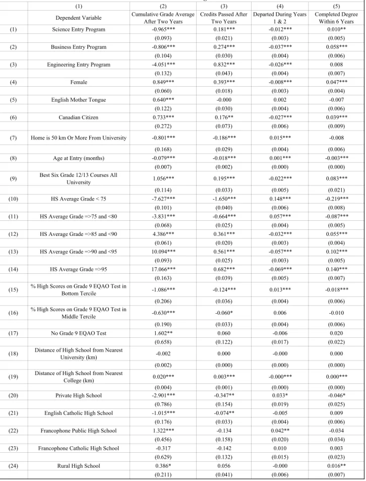
We report estimates of a simple regression model of each of our four outcomes in Table 3.15 Each
regression also contains a dummy variable for each university the estimates of which are not included in this paper due to confidentiality considerations. We begin with the coefficients for individual characteristics in the first regression (cumulative GPA after two years) in column 2. The finding that stands out is the importance of the student’s high school grade average. Students in the lowest and highest high school grade categories have university grade averages that differ by about 25 percentage points. The most noticeable difference by program is that Engineering students have cumulative grade averages that are 3 to 4 percentage points lower than those of other students.
15 We also estimated models for credits completed and cumulative grade average at the end of Year 1, the likelihood of a departure during Year 1, and degrees completed within four or five years after entry. The estimated coefficients were quite robust across different measures of the same outcome. The major exception was the differences among academic programs in the length of time to complete a degree.
10
The differences in university grades associated with the other individual characteristics are often statistically significant but numerically small. Students who are female, whose mother tongue is English, who are Canadian citizens and whose best six high school courses are all university stream have higher university grades. “Commuters” do slightly better than those living more than 50 km from campus. Those aged 20 do slightly worse than those aged 19 which may reflect a so-called “victory lap” phenomenon, that is, students who take an extra year of high school to improve grades.
We next turn to the coefficients for high school characteristics in column 2. The difference in cumulative grade averages between students from high schools with average standardized math scores (the Grade 9 Math Assessment) in the bottom tercile and those in the top tercile is only 1 percentage point. Students from schools with no standardized math scores do slightly better.16 All else equal,
students from privately funded high schools have university grade averages that are 3 percentage points lower than those from the omitted category (publicly funded English schools).17 Students from English
Catholic high schools do worse, and those from Francophone public schools do a bit better, than those from English public schools, but these are small differences of 1 percentage point or less. The same is true of the superior performance of students from schools in rural areas.
The coefficients for neighbourhood characteristics in column 2 of Table 3 indicate that the difference in cumulative grade averages between students from low income and high income neighbourhoods is less than 1 percentage point and statistically insignificant. The estimated impact of other neighbourhood characteristics is equally small even when statistically significant. In summary, most of the differences in university grades in Column 2 of Table 3 are quite small save for those by
16 For purposes of estimating these regressions, students from high schools with missing standardized math scores were included in the group of students from high schools with average scores in the middle tercile. We also estimated the regressions excluding students from high schools for which standardized math scores were missing and the resulting coefficients were very similar to those in Table 3.
17 A systematic analysis of differences between students from privately funded and publicly funded high schools is beyond the scope of this paper but our suspicion is that the students from privately funded schools are a very heterogeneous group. At a minimum in such an analysis, one would need to account for the fact that most private schools did not have their students take the standardized Math Assessment.
11
high school grade averages. Although these small estimated effects of other individual, high school and neighbourhood characteristics condition on high school grades, we find that these estimated effects remain similarly small if the high school grade average variables are dropped from the model (not shown here). The same is true of the remaining estimates in Table 3.
Column 3 of Table 3 contains the coefficients from the second regression in Table 3 in which the dependent variable is the cumulative credits passed two years after entry. The pattern of coefficients is quite similar to that in column 2. Once again, the individual characteristic that stands out most is high school grade average. At the end of two years, students in the lowest high school grade category have earned 2.4 fewer credits (almost a half a year less) than those in the highest high school grade category. The most noticeable difference among programs is that Engineering students have earned almost 0.5 to 0.8 of a credit more than other students.18 Females have 0.4 credits more than males. The differences
in credits passed associated with the remaining individual characteristics are quite small even when statistically significant. One difference from column 2 is that English mother tongue is not associated with more credits passed in column 3. The estimated effects of high school and neighbourhood characteristics in column 3 are very small. For example, the differences between students from high schools in the bottom and top terciles of standardized math scores is only about one-tenth of a credit which is also the difference between students from low- and high-income neighbourhoods.
Column 4 of Table 3 contains the coefficients from the third regression in which the dependent variable is a departure in years one or two after entry. The signs of the coefficients are generally the opposite of those in columns 2 and 3 because a departure is often a “bad” academic outcome. The basic message of column 4 is quite similar to that of the previous two columns. Most importantly, students in the lowest high school grade category have a departure rate that is almost 21 percentage points higher than those in the highest high school grade category. Commerce students have the lowest departure rate
18
12
and it is 4 percentage points lower than that of students in Arts (controlling for other factors including high school grades). The female departure rate is less than 1 percentage point lower than that of males. Individual characteristics, such as holding Canadian citizenship and taking all university courses, are associated with departure rates that are about 2 percentage points lower. In column 4, private schools and Francophone public high schools are associated with substantially higher departure rates (about 4 percentage points) but Catholic and rural schools are not. This difference in departure rates between students from low-standardized math and high-standardized math high schools is only 1 percentage points. The same is true of the difference between students from low-income and high-income neighbourhoods. Other neighbourhood characteristics have similarly small impacts.
Column 5 of Table 3 charts the coefficients from the fourth regression in which the dependent variable is degree completion within six years. The qualitative pattern of coefficients is generally similar to that in the previous columns. The students in the lowest high school grade category have a degree completion rate that is 36 percentage points lower than those in the highest high school grade category. Commerce students have a degree completion rate that is 5 to 6 percentage points higher than that of students in other programs. The female completion rate is almost 5 percentage points higher than that of males. Canadian citizenship is associated with an increase in the likelihood of degree completion of 4 percentage points.19 Taking all university courses predicts a degree completion rate that is between
8 and 9 percentage points higher. Students from private high schools have lower completion rates (almost 5 percentage points) and students from rural high schools have slightly higher completion rate (about 2 percentage points). Other high school characteristics have small impacts as do the neighbourhood characteristics in column 5. For example, the difference in completion rates between students from high schools in the bottom and top terciles of standardized math scores or between students from low- and high-income neighbourhoods is only about 2 percentage points.
19 This impact of citizenship on departures and degree completion may in part reflect a difference between first- and second- generation immigrants as found by Finnie, Childs and Qiu with the Youth In Transition Survey data (2010).
13
Each of our regressions contained a dummy for each of our four universities (not shown for confidentiality reasons) and for each entry year. The coefficient estimates for these variables yield conclusions very similar to those that we drew from the trends in mean outcomes in Figure 1 in the following two ways. First, the differences among our four universities are small and their rank order changes. Second, the levels of our persistence measures have generally been quite stable. The one difference from the trends in Figure 1 is that the year coefficients in Table 3 indicate only a very minor improvement in the departure rate for the “double cohort” that entered in 2003. This difference is likely due to the fact that the regressions control for the high school grade averages of entering students.
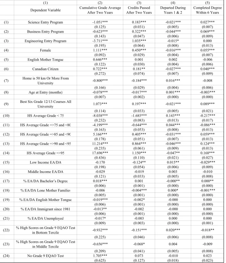
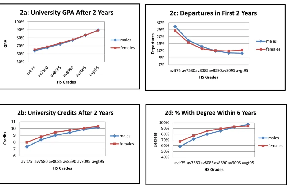
We also estimated a set of four regressions that contain interactions between high school grades and the following variables: gender, program, neighbourhood average income and high school average standardized math performance. These interaction effects are illustrated in Figures 2 through 5. The coefficients for variables that were not interacted with high school grades are very similar to those in Table 3 and the full set of estimates is available upon request. (These regressions have been included for the editor and referees in Table A-2.) Figures 2a through 2d present the relationships between high school grade average and each of our outcomes for both males and females. In each figure, we started with the sample mean or proportion of the dependent variable in our sample for males with a high school grade average in the range from 80 to 85 and then drew the figures using the estimated regression coefficients to calculate the estimated values for the other high school grade averages.20
Figures 2a through 2d indicate that the strong relationship between high school grade category and university outcomes is true of both sexes. Females have better university outcomes for most of the measures among students with low high school grades. For example, among students with a high school average of less than 75, the female departure rate is 3 percentage points lower than that of males and the female degree completion rate is 9 percentage points higher. The performance levels of females and
20 We centered the figures in the 80 to 85 grade range because this contains the sample mean (83.4). This same approach was used in Figures 3 through 5.
14
males converge or even reverse as one considers better high school grade averages. Among students with a high school average of 95 or better, for example, the female departure rate is 2.5 percentage points higher than that of males and the female degree completion rate is 3 percentage points lower.21
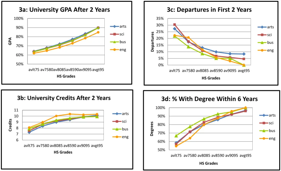
Figures 3a through 3d show the relationship between high school grade averages and university outcomes by entry program. Figures 3a and 3b show that Engineering students have lower grade averages and more credits completed after two years than students in other programs, regardless of high school grade category. Figures 3c and 3d indicates that Business students have the lowest departure rates and the highest degree completion rates in most grade categories.
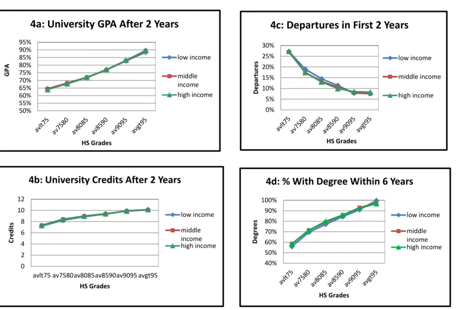
Figures 4a through 4d show the relationship between high school grade averages and university outcomes by neighbourhood average equivalent income tercile. In Figures 4a and 4b, the differences between students from low income and high income neighbourhoods in university grades are 1 percentage point or less and the differences in credits completed are 0.2 credits or less for each high school grade category. Departure rates in Figure 4c show slightly larger differences but even these are at most 1.5 percentage points. Similarly the differences in degree completion rates between low- and high-income students in Figure 4d are at most 3 percentage points. Differences in both departure and degree completion rates are a bit larger at low high school grade levels but the key message of Figure 4 is that neighbourhood income does not have a substantial link with our outcomes, regardless of high school grade average.
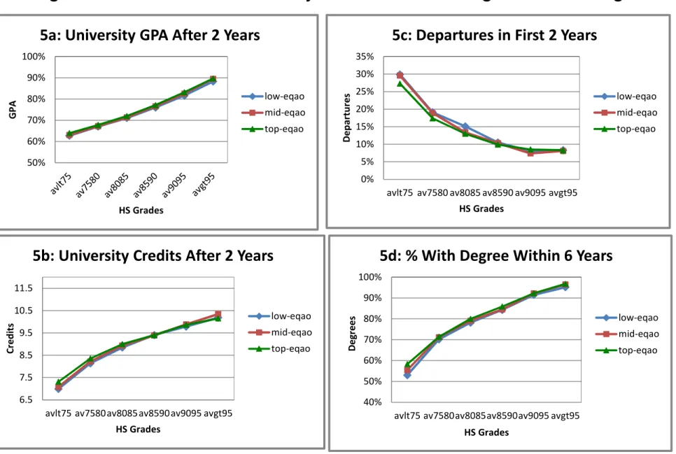
Finally, Figures 5a through 5d show the relationship between high school grade averages and university outcomes by the average performance of the student’s high school on the academic Grade 9 standardized math test. In Figures 5a and 5b, the differences in university grade averages between individuals from schools with the smallest proportion of high standardized math scores and those from schools with the largest proportion of high standardized math scores are all 1.5 percentage points or less
21 In this and the next four charts,the slopes of the line segments indicate the ‘importance’ of better high school grades, while the differences in heights indicate the ‘importance’ of the other variable.
15
and the differences in credits completed are all 0.3 credits or less. The same differences in departure rates in Figure 5c are at most 2 percentage points and the differences in degree completion rates in Figure 5d are at most 3 percentage points. As with differences by neighbourhood income, the differences by high school standardized math performance are somewhat larger at lower high school grade averages but overall are quite small.
The general message of Table 3 and Figures 2 through 5 is that neighbourhood, high school and individual characteristics other than high school GPA have relatively weak links with our measures of persistence and success in university. Table 4 provides an illustration of the relative importance of the different sets of independent variables in our regressions. We use our estimated regression coefficients (from the specification with interactions) to predict our four academic outcomes for students from three different types of families. As indicated by Table 4a, we define a “disadvantaged student” as being from the following background: high school standardized math scores and neighbourhood average equivalent income are in the bottom terciles for the province; the proportion of adults with a Bachelor’s degree and the proportion of families with the home language of English are at the 25th percentiles; and the unemployment rate, the proportion of families headed by a lone mother and the proportion of adults who are recent immigrants are at the 75th percentiles. An “average student” is from the following
background: high school standardized math scores and average equivalent income are in the middle terciles; and the proportion of adults with a Bachelor’s degree, the proportion of families with the home language of English, the unemployment rate, the proportion of families headed by a lone mother and the proportion of adults who are recent immigrants are all at the 50th percentiles. An “advantaged student”
is from the following background: high school standardized math scores and average equivalent income are in the top terciles; the proportion of adults with a Bachelor’s degree and the proportion of families with the home language of English are at the 75th percentiles; and the unemployment rate, the proportion of families headed by a lone mother and the proportion of adults who are recent immigrants
16
are at the 25th percentiles. These predicted values assume the omitted category for the remaining binary
variables in the regression and mean sample values for the remaining continuous variables.
Most of the entries in Table 4b are predicted values of each of our outcomes. Rows 7 and 14 present the differences in outcomes between students in the top and bottom high school grade categories. Columns 4 and 8 contain the differences in outcomes between advantaged and disadvantaged students. The most striking pattern is that the absolute differences by high school GPA are much larger than the absolute differences by high school and neighbourhood advantage. However, there are also some interesting variations by university outcome. The entries in column 4 indicate that the difference in university GPA between advantaged and disadvantaged students is only 1.2 percentage points for those with the a high school GPA of 75 or less but is 3.2 percentage points among students with a high school GPA of 95 and above. The opposite is seen for the three other university outcomes, that is, the differences between advantaged and disadvantaged students are smaller among students with better high school grades especially in the case of degree completion. For example, column 8 shows that the difference between advantaged and disadvantaged students in the likelihood of completing a degree is 9 percentage points for those with a high school GPA of 75 or less but is only 1 percentage point for those with a high school GPA of 95 or higher.
In Table 4c, we explore further the differences in the four persistence measures as we move across the high school marks gradient. Rows 15 through 24 report the incremental change in the outcome measure as we move from lower to higher high school marks. For instance, the entry in row 15, column 1 indicates that the predicted university GPA increases by 3.7 percentage points when one compares a disadvantaged student in the 75 or less HS grade category with a disadvantaged student in 75 to 80 HS grade category. (This is row 2 minus row 1 in column 1 of Table 4b.) This difference is larger at higher HS grade levels regardless of socioeconomic status. For instance, the entry in row 19, column 1 indicates that the predicted university GPA increases by 6.1 percentage points when one
17
compares a disadvantaged student in the 90-95 HS grade category to a disadvantaged student in 95 or better HS grade category.
As in Table 4b, the pattern is different for the other outcomes especially the likelihoods of departure and degree completion. For example, the entry in row 20, column 1 indicates that the likelihood of a departure decreases by 8 to 10 percentage points (depending on socioeconomic status) when one moves from a student in the 75 or less HS grade category to a student in 75-80 HS grade category. In contrast the differences between students in the 90-95 HS grade category and the 95 or better HS grade category are only 1 to 2 percentage points. The entry in row 20, column 5 indicates that the likelihood of degree completion increases by 12 to 16 percentage points (depending on socioeconomic status) when one moves from a student in the 75 or less HS grade category to a disadvantaged student in 75-80 HS grade category. In contrast the differences between students in the 90-95 HS grade category and the 95 or better HS grade category are only 4 to 7 percentage points. We comment on the policy implications of Table 4 in the next section.
We also explored the robustness of our findings using several alternative regression specifications. First, we checked the stability of the high school GPA effect over time by interacting the high school grade variables with a binary variable for the second half of our data period (1999-2005). All of these interaction coefficients were small in size and almost all were not significantly different from zero. The same was true when we divided our sample period into thirds. Hence, the relationship between high school grades and our university outcomes appears to be stable over time.
Second, we investigated the explanatory power of different sets of independent variables. Row 1 of Table 5 contains the (adjusted) R squared values from Table 3. Row 2 shows that the omission of all neighbourhood and school characteristics leads to little no decrease in the R-squared. For Row 3, we omitted the individual characteristics, including high school grades, which leads to a substantial decline in the R squared. The specification in Row 4 omitted only high school grades and the declines in the R
18
squared are almost as large as in Row 3. Hence, high school GPA is the clearly most important single variable in terms of accounting for variation in our university outcomes.
Third, we assessed the possibility that our school and neighbourhood variables do not capture those characteristics which are most relevant for success in university. The model estimated for Row 5 of Table 5 included a fixed effect for each high school in our sample along with the individual and neighborhood characteristics. The inclusion of the high school fixed effects does increase the R-squared somewhat indicating that there are some relevant characteristics of these high schools that the variables in our current data set do not capture. The differences in R square between Row 1 and 5, however, are quite modest indicating that unmeasured school characteristics captured by our fixed effects model do not add a great deal of explanatory power. Moreover, the coefficients and standard errors for the individual and neighbourhood variables in the school fixed effects model area very similar to those in Table 3.22
For the model in Row 6, we included a fixed effect for each Enumeration/Dissemination Area in our sample along with the individual and high school variables. Here too, the R-squared statistics in Row 6 are higher than those in Row 1 but the differences are modest indicating that unmeasured neighbourhood characteristics captured by our fixed effects model do not substantially increase the explanatory power of the model. There is also little change in the coefficients for the individual and high school variables in the neighbourhood fixed effects model. These estimates imply that there are not fixed (and unmeasured) characteristics of the high schools and neighbourhoods in our sample that would greatly increase our ability to account for the variation in university outcomes.23
22 We ranked the students (schools) in our sample by estimated high school fixed effect. The differences between students at the 75th and 25th percentiles are the following: 2.4 (2.3) percentage points in Year 1 and 2 GPA; 0.5 (0.6) credits completed by end of Year 2; 7 (8) percentage points in the likelihood of a departure in Years 1 and 2; and 7 (11) percentage points in the likelihood of degree completion within six years. These estimated high school fixed effects have not been corrected for sampling error and hence likely overstate the differences in true high school fixed effects.
23We also ranked the students (neighbourhoods) in our sample by estimated neighbourhood fixed effects. The differences
between students at the 75th and 25th percentiles are the following: 3.8 (5.3) percentage points in Year 1 and 2 GPA; 0.9 (1.4) credits completed by end of Year 2; 14 (19) percentage points in the likelihood of a departure in Years 1 and 2; and 16 (25)
19 6. Policy Discussion and Conclusion
We have used a unique set of linked data sets to examine the correlates of four measures of persistence and success in university: cumulative grade averages, credits completed and departures during the first two years, and degrees completion within six years. Our key empirical findings are two. First, high school grade point average is strongly linked to all of our university outcomes in the sense of both the magnitude and the precision of the estimated regression coefficients. Second, the neighbourhood and high school characteristics used in this study, such as average neighbourhood income and the average Grade 9 Math Assessment scores of a high school, have weak links with university outcomes. The explanatory power of the high school grades greatly dominates that of other variables considered individually or jointly.
We believe that two important, albeit tentative, policy conclusions can be drawn from our findings. First, there is a positive message regarding the educational system in Ontario. Students in our sample from disadvantaged neighbourhoods and high schools with weaker performance on standardized tests are as well prepared for university as students with the same individual high school grades but from advantaged neighbourhoods and higher performing high schools. Viewed from the university perspective, the positive message is that these four institutions provide an environment in which students with similar high school grades but otherwise heterogeneous backgrounds have very similar likelihoods of success. Of course, it might be that a different set of neighbourhood and high school variables would have much better explanatory power and yield different conclusions. Our estimates with fixed effect models for both high schools and neighbourhoods, however, do not indicate that this would be the case. Second, students with the lowest high school grades in our sample have a very low probability of completing a degree at these four universities and are much less likely to do so than students with
percentage points in the likelihood of degree completion within six years. These estimated neighbourhood fixed effects have not been corrected for sampling error and hence likely overstate the differences in true neighbourhood fixed effects.
20
slightly better high school grades. This provides a clear note of caution regarding a policy of improving access to the university system by reducing the minimum grade average required for admission.
Our findings also suggest several fruitful opportunities for future policy research. In contrast with the findings of the current paper, we reported in Dooley, Payne and Robb (2009) that neighbourhood and high school measures have substantial links with the decision to apply to and register in university. Students from low income neighbourhoods are 14 percentage points less likely to apply to or register in university than those in high income neighbourhoods (controlling for other factors including high school grades). Students from high schools in which fewer than 50% of students attained a high standardized math score (3 or 4) were 8 percentage points less likely to apply to or register in university than students in high schools in which more than 50% received a high standardized math score (controlling for other factors including GPA). Furthermore, the period from 1994 through 2006 saw no decrease in these differences in application and registration rates and perhaps even a slight increase. The findings in our two papers indicate that future research should be devoted to the analysis of students from less advantaged high schools and neighbourhoods who do not apply to university. What proportion of such non-applicants or non-registrants have high school grades that would predict a reasonable likelihood of success in university? What appear to be barriers other than grades to their access to the university system?
The key role of high school grades in our findings begs the question of what lies behind the variation in high school grades. What is the role of variation in socio-economic characteristics among families within neighbourhoods? How important is variation in the secondary programs followed by students? Further linkage with individual student information on family income and high school academic programs could shed further light on the determinants of both strong high school grade average and success in university.
Finally, our results highlight the advantages of administrative data for policy research. Such data suffer much less than do survey data from errors in reporting and recall, and from response and selection bias. We have students’ actual grades rather than self-reports and close to full coverage of the relevant
21
populations rather than just responses to a voluntary survey. In addition, our sample size is very large even with only four universities. Efforts to extend our sample to other universities and to link with administrative data sets from colleges and secondary schools should definitely be pursued.
References
Bowlby, Jeffrey and Kathryn McMullen. (2002). “At a Crossroads: First Results for the 18 to 20 Year old Cohort of the Youth in Transition Survey.” Ottawa: Human Resources Development Canada and Statistics Canada.
Chemin, Matthieu. (2009). “Does student financial aid cause more participation in and graduation from post-secondary education?” MESA Project Research Paper. Toronto, ON: Educational Policy Institute.
Conrad, Mark and Katherine Morris. (2010). “Shifting from Retention Rates to Retention Risk: An Alternative Approach for Managing Institutional Student Retention Performance”. Toronto: Higher Education Quality Council of Ontario.
Dooley, Martin, A. Abigail Payne and A. Leslie Robb. (2009). “University Participation and Income Differences: An Analysis of Applications by Ontario Secondary School Students.” Toronto, ON: Higher Education Quality Council of Ontario.
Dooley, Martin, A. Abigail Payne and A. Leslie Robb. (2011). “Understanding the Determinants of Persistence and Academic Success in University: An Exploration of Data from Four Ontario Universities.” Toronto, ON: Higher Education Quality Council of Ontario.
Finnie, Ross and Theresa Qiu. (2008). “Is The Glass (or Classroom) Half-Empty or Nearly Full? New Evidence on Persistence in Post-Secondary Education in Canada.” In Finnie, R., R.E. Mueller, A. Sweetman and A. Usher (Eds.), Who Goes? Who Stays? What Matters? Accessing and Persisting in Post-Secondary Education in Canada, pp. 179-208. Montreal and Kingston: McGill-Queens University
Press.
Finnie, Ross and Theresa Qiu. (2009). “Moving Through, Moving On: Persistence in Post-Secondary Education in Atlantic Canada, Evidence from the PSIS.” Ottawa: Statistics Canada, Centre for Education Statistics Research Papers.
Finnie, Ross, Stephen Childs and Theresa Qiu. (2010). “Patterns of Persistence in Postsecondary
Education: New Evidence for Ontario.” The Education Policy Research Initiative, University of Ottawa. Grayson, J. Paul and Kyle Grayson. (2003). “Research on Retention and Attrition.” Montreal: Canadian Millennium Scholarship Foundation.
Johnson, David. (2008). “How is Variation in Tuition Across Canadian Provinces Related to University Participation in the Youth in Transition Survey?” In Finnie, R., R.E. Mueller, A. Sweetman and A. Usher (Eds.), Who Goes? Who Stays? What Matters? Accessing and Persisting in Post-Secondary Education in Canada, pp299-326. Montreal and Kingston: McGill-Queens University Press.
Martinello, Felice. (2008). “Transitions and Adjustments in Students’ Canadian Post-Secondary Education.” In Finnie, R., R.E. Mueller, A. Sweetman and A. Usher (Eds.), Who Goes? Who Stays? What Matters? Accessing and Persisting in Post-Secondary Education in Canada, pp. 209-238.
Montreal and Kingston: McGill-Queens University Press.
Mueller, Richard E. (2008a). “Access and Persistence of Students in Canadian Post-Secondary Education: What We Know, What We Don’t Know and Why It Matters.” In Finnie, R., R.E. Mueller, A.
Sweetman and A. Usher (Eds.), Who Goes? Who Stays? What Matters? Accessing and Persisting in Post-Secondary Education in Canada, pp. 33-62. Montreal and Kingston: McGill-Queens University
2
Mueller, Richard E. (2008b). “Access and Persistence of Students from Low-Income Backgrounds in Canadian Post-Secondary Education: A Review of the Literature.” MESA Project Research Paper
2008-1. Toronto, ON: Educational Policy Institute.
Nory, Amaury, Elizabeth Barlow, and Gloria Crisp. (2005). “Student Persistence and Degree Attainment Beyond the First Year in College: The Need for Research.” In Seidman, Alan (Ed.), College Student Retention: Formula for Student Success, pp. 145-166. Westport, CT: Praeger Publishers
Ontario Ministry of Training, Colleges and Universities (2010). “Key Progress Indicators for Universities.”
Parkin, Andrew, and Noel Baldwin (2009). “Persistence in Postsecondary Education in Canada: The Latest Research”, Research Note #8. Montreal: Canada Millennium Scholarship Foundation.
Table 1
Students Applying and Registering Directly From An Ontario High School: 1999-2004*
Total OUAC
Applicants Ontario Universities Total Registrants in Persistence Data Number of Students 426,594 298,697 83,496
% of OUAC Applicants 100% 70% 20%
% of Ontario University
Registrants 143% 100% 28%
% Female 55.9% 57.9% 56.5%
% English mother tongue 78.7% 79.8% 84.6%
% Canadian citizen 89.9% 91.5% 93.1%
Mean Age at Entry 19.4 19.1 18.5
Mean grade in best six
Grade 12/OAC courses 78.5 81.3 83.4
Mean Grade OAC/Grade 12
core English course 76.4 78.5 80.1
*The years 1999 through 2004 are those for which we have data for entering classes from all four universities in our data.
(1) (2) (3) (4) (5) Grade Point after
2 years Mean Credits after 2 years
% Departed during Years 1 and 2 % Any Degree within 6 years Total 72 9.2 13% 80% Arts 70 8.7 17% 75% Science 73 9.1 12% 81% Business 73 9.4 9% 88% Engineering 72 9.7 9% 82% Male 71 8.9 13% 77% Female 72 9.2 13% 82% <75 63 7.4 28% 58% =>75 and <80 67 8.4 19% 72% =>80 and <85 70 9.1 12% 81% =>85 and <90 74 9.5 9% 87% =>90 and <95 79 9.7 6% 91% =>95 86 9.9 5% 94% Bottom Tercile 71 8.9 15% 77% Middle Tercile 72 9 13% 80% Top Tercile 72 9.1 12% 81% Bottom Tercile 71 9 14% 78% Middle Tercile 72 9.2 13% 80% Top Tercile 72 9.2 12% 81% Number of Observations 113,271 113,271 97,558 55,574
Number of Years Observed 2 or more years 2 or more years 3 or more years 6 or more years
Table 2 Summary Statistics for Measures of Persistence by Entry Program,
By Proportion of Students Achieving High Score (3 or 4) on Academic EQAO Test By Neighborhood Average Equivalent Income
By High School Grade Point Average By Gender
By Entry Program
(1) (2) (3) (4) (5) Dependent Variable Cumulative Grade Average After Two Years Credits Passed After Two Years Departed During Years 1 & 2 Completed Degree Within 6 Years (1) Science Entry Program -0.965*** 0.181*** -0.012*** 0.010**
(0.093) (0.021) (0.003) (0.005) (2) Business Entry Program -0.806*** 0.274*** -0.037*** 0.058***
(0.104) (0.030) (0.004) (0.006) (3) Engineering Entry Program -4.051*** 0.832*** -0.026*** 0.008
(0.132) (0.043) (0.004) (0.007) (4) Female 0.849*** 0.393*** -0.008*** 0.047***
(0.060) (0.018) (0.003) (0.004) (5) English Mother Tongue 0.640*** -0.000 0.002 -0.007 (0.122) (0.030) (0.004) (0.006) (6) Canadian Citizen 0.733*** 0.176** -0.027*** 0.039***
(0.272) (0.073) (0.006) (0.009) (7) Home is 50 km Or More From University -0.801*** -0.186*** 0.015*** -0.008 (0.168) (0.029) (0.004) (0.006) (8) Age at Entry (months) -0.079*** -0.018*** 0.001*** -0.003***
(0.007) (0.002) (0.000) (0.000) (9) Best Six Grade 12/13 Courses All University 1.056*** 0.195*** -0.022*** 0.083***
(0.114) (0.033) (0.005) (0.021) (10) HS Average Grade < 75 -7.627*** -1.650*** 0.148*** -0.219***
(0.101) (0.040) (0.006) (0.008) (11) HS Average Grade =>75 and <80 -3.831*** -0.664*** 0.057*** -0.087***
(0.068) (0.025) (0.004) (0.005) (12) HS Average Grade =>85 and <90 4.386*** 0.361*** -0.032*** 0.055***
(0.061) (0.020) (0.003) (0.004) (13) HS Average Grade =>90 and <95 10.094*** 0.561*** -0.057*** 0.102***
(0.093) (0.025) (0.003) (0.005) (14) HS Average Grade =>95 17.066*** 0.682*** -0.069*** 0.140***
(0.163) (0.039) (0.005) (0.007) (15) % High Scores on Grade 9 EQAO Test in Bottom Tercile -1.086*** -0.124*** 0.013*** -0.018***
(0.206) (0.036) (0.004) (0.006) (16) % High Scores on Grade 9 EQAO Test in Middle Tercile -0.630*** -0.060* 0.006 -0.010 (0.190) (0.033) (0.004) (0.006) (17) No Grade 9 EQAO Test 1.602** 0.060 -0.006 0.020
(0.658) (0.122) (0.017) (0.022) (18) Distance of High School from Nearest University (km) -0.002 0.000 -0.000 0.000
(0.002) (0.000) (0.000) (0.000) (19) Distance of High School from Nearest College (km) 0.020*** 0.003*** -0.000*** 0.000***
(0.004) (0.001) (0.000) (0.000) (20) Private High School -2.901*** -0.347** 0.033* -0.046* (0.786) (0.154) (0.019) (0.025) (21) English Catholic High School -1.015*** -0.074** -0.005 0.009
(0.176) (0.033) (0.004) (0.006) (22) Francophone Public High School 1.322*** -0.134 0.042** -0.034 (0.456) (0.158) (0.020) (0.034) (23) Francophone Catholic High School -0.317 -0.142 0.010 0.003
(0.629) (0.132) (0.015) (0.023) (24) Rural High School 0.386* 0.056 -0.000 0.016** (0.211) (0.041) (0.006) (0.007) Table 3 Multivariate Regressions
(25) High School Enrolment in Bottom Tercile -1.015*** -0.168*** 0.020*** -0.019*** (0.240) (0.046) (0.005) (0.007) (26) High School Enrolment in Middle Tercile -0.460** -0.052* 0.011*** -0.007 (0.193) (0.031) (0.004) (0.005) (27) Low Income EA/DA -0.159 -0.077* 0.010** -0.020***
(0.165) (0.040) (0.005) (0.007) (28) Middle Income EA/DA -0.002 0.003 0.002 -0.003 (0.099) (0.023) (0.003) (0.005) (29) % EA/DA Bachelor’s Degree 0.018*** 0.001 -0.000** 0.000** (0.006) (0.001) (0.000) (0.000) (30) % EA/DA Lone Mother Families -0.006 -0.004*** 0.000 -0.001***
(0.006) (0.001) (0.000) (0.000) (31) % EA/DA English Mother Tongue -0.019*** -0.002 -0.000 0.000
(0.006) (0.001) (0.000) (0.000) (32) % EA/DA Immigrant since 1981 -0.014** -0.002 -0.000 0.000
(0.006) (0.001) (0.000) (0.000) (33) % EA/DA Unemployed -0.018** -0.003 0.000 0.000 (0.009) (0.002) (0.000) (0.001) (34) 1995 Entry Year -0.347** -0.083* 0.017*** -0.020*** (0.135) (0.047) (0.006) (0.007) (35) 1996 Entry Year -0.217 -0.024 0.006 -0.009 (0.145) (0.049) (0.006) (0.007) (36) 1997 Entry Year 0.059 0.026 -0.004 -0.005 (0.143) (0.049) (0.007) (0.008) (37) 1998 Entry Year 0.228 0.063 -0.001 -0.005 (0.143) (0.046) (0.006) (0.007) (38) 1999 Entry Year 0.251* -0.058 -0.001 -0.004 (0.137) (0.045) (0.006) (0.007) (39) 2000 Entry Year 0.324** 0.022 -0.008 -0.007 (0.150) (0.048) (0.006) (0.009) (40) 2001 Entry Year 0.444*** 0.043 -0.007 -0.017 (0.155) (0.048) (0.006) (0.010)
(41) 2002 Entry Year 0.394*** 0.047 -0.006 n.a.
(0.151) (0.043) (0.006)
(42) 2003 Entry Year 0.229 -0.082* -0.017** n.a.
(0.161) (0.046) (0.007)
(43) 2004 Entry Year -0.805*** -0.225*** 0.005 n.a.
(0.212) (0.055) (0.009)
(44) 2005 Entry Year -0.834*** -0.179*** n.a. n.a. (0.232) (0.060)
(45) Constant 89.757*** 13.320*** -0.129*** 1.338***
(1.474) (0.416) (0.049) (0.081)
Observations 113,271 113,407 97,558 55,574
R-squared 0.380 0.113 0.042 0.073
Sample mean or proportion 72 9.2 13% 80%
Clustered standard errors in parentheses, *** p<0.01, ** p<0.05, * p<0.1
Constant (reference group) is for a male, Arts, non-English mother tongue, not a citizen, resides within 50 km, some non-University courses, GPA 80-85, high income, top tercile EQAO scores, 1994 entry. High school is publicly funded, English, public, Anglophone and urban. Each regression also contains a dummy variable for each university.
Characteristics Value Characteristics Value Characteristics Value
Low - Medium - Top
-Low - Medium - Top
-25th Percentile 7.7 50th Percentile 14.6 75th Percentile 25.8 75th Percentile 17.4 50th Percentile 10.5 25th Percentile 5.7 25th Percentile 86.1 50th Percentile 95.7 75th Percentile 100.0 75th Percentile 18.1 50th Percentile 5.8 25th Percentile 1.5 75th Percentile 8.6 50th Percentile 5.3 25th Percentile 2.9
(1) (2) (3) (4) (5) (6) (7) (8)
Disadvantaged Average Advantaged (3) - (2) Disadvantaged Average Advantaged (7) - (5)
(1) HS GPA<75 61.5 62.1 62.7 1.2 7.0 7.2 7.5 0.5 (2) HS GPA 75-80 65.2 66.0 66.4 1.2 8.0 8.3 8.4 0.4 (3) HS GPA 80-85 68.6 69.3 70.5 1.9 8.9 9.0 9.1 0.2 (4) HS GPA 85-90 73.1 73.8 75.0 1.9 9.2 9.3 9.4 0.2 (5) HS GPA 90-95 78.4 79.6 80.8 2.5 9.4 9.5 9.5 0.1 (6) 95+ 84.5 87.1 87.7 3.2 9.5 9.7 9.6 0.1 (7) (6) - (1) 23.0 25.0 25.0 2.5 2.5 2.1 (8) HS GPA<75 27% 26% 24% -3% 35% 41% 44% 9% (9) HS GPA 75-80 18% 17% 15% -3% 51% 55% 56% 4% (10) HS GPA 80-85 11% 11% 10% -2% 61% 63% 65% 4% (11) HS GPA 85-90 9% 8% 7% -2% 66% 68% 70% 4% (12) HS GPA 90-95 4% 4% 6% 1% 71% 74% 74% 3% (13) 95+ 3% 3% 4% 1% 77% 77% 78% 1% (14) (12) - (7) -23% -23% -20% 42% 36% 34% (1) (2) (3) (5) (6) (7)
Disadvantaged Average Advantaged Disadvantaged Average Advantaged
(15) HS GPA 75-80 vs. <75 3.7 3.9 3.7 1.0 1.1 0.9
(16) HS GPA 80-85 vs. 75-80 3.4 3.3 4.1 0.9 0.7 0.7
(17) HS GPA 85-90 vs. 80-85 4.5 4.5 4.5 0.3 0.3 0.3
(18) HS GPA 90-95 vs. 85-90 5.3 5.8 5.8 0.2 0.2 0.2
(19) HS GPA 95+ vs. 90-95 6.1 7.5 6.9 0.1 0.2 0.1
Disadvantaged Average Advantaged Disadvantaged Average Advantaged
(20) HS GPA<75 -8% -10% -9% 16% 14% 12% (21) HS GPA 75-80 -7% -6% -5% 10% 9% 10% (22) HS GPA 80-85 -3% -3% -3% 5% 5% 5% (23) HS GPA 85-90 -4% -4% -1% 5% 6% 4% (24) HS GPA 90-95 -1% -1% -2% 7% 3% 4% % Recent Immigrants Disadvantaged Average
% Lone Mother Families % with English as Home Lang.
Advantaged
Table 4a: Characteristics of Different Family Types
High School EQAO Tercile Neighbourhood Income Tercile
% with Bachelors Degree
% Unemployment Rate
Table 4b: Predicted University Outcomes for Different Family Types
Predicted Year 1 & 2 University GPA Predicted Year 1 & 2 Accumulated Credits
Predicted Likelihood Year 1 & 2 Departure Predicted Likelihood of Degree in 6 Years
Table 4c: Differences in Predicted University Outcomes by HS GPA for Different Family Types
Predicted Year 1 & 2 University GPA Predicted Year 1 & 2 Accumulated Credits
Table 5
Adjusted R Squared in Various Specifications of Basic Model with No Interactions GPA after 2
years Credits after 2 years Departure during Likelihood Years 1 and 2
Likelihood Degree after 6
Years
(1) Table 3 regression estimates 0.38 0.11 0.04 0.07
(2) No high school or neighbourhood
characteristics 0.37 0.11 0.04 0.07
(3) No individual characteristics 0.04 0.04 0.01 0.02
(4) No high school grades 0.06 0.06 0.02 0.03
(5) School Fixed Effect with individual
and neighbourhood characteristics 0.41 0.13 0.05 0.08
(6) Neighbourhood Fixed Effect with
individual and school characteristics 0.40 0.13 0.06 0.09
Table A-1
Definition and Sample Means or Proportions of Variables
Variable Name Definition: All Binary Variables Unless Otherwise Indicated (“Year” refers to the twelve-month period following September entry)
Sample Mean or Proportion Panel A: University Administrative Variables
Arts Entry Program Enrolled in an Arts program in Year 1. 41% Science Entry Program Eenrolled in a Science program in Year 1. 35% Business Entry
Program Enrolled in a Business program in Year 1
12% Engineering Entry
Program Enrolled in a Engineering program in Year 1.
12% Cumulative GPA Years
1 & 2
Cumulative grade point average at the end of year 2 among students
observed for 2 or more years. 72
Cumulative Credits Passed Years 1 & 2
Cumulative credits passed at the end of year 2 among students observed for 2
or more years. 9.2
% Departed During Years 1 & 2
Proportion of students for whom we observe only missing values in the third
calendar year after entry among students observed for 3 or more years. 13% % with Degree after 6
Years
Proportion of students for whom we observe a degree earned at the end of 6
years after entry among students that we observe for 6 or more years. 80% Panel B: Ontario Universities Application Centre Variables
Female Student is female. 57%
English Mother Tongue Student’s mother tongue is English. 85% Canadian Citizen Student is a Canadian citizen. 93% Distance to Campus Home is more than 50 km from campus. 6% Age at Entry Age (in months) at entry to university 222 Average HS Grade< 75 Average grade is less than 75 (mostly greater than 70). 9% Average HS Grade
>=75 and <80 Average grade is equal to or greater than 75 and less than 80.
18% Average HS Grade
>=80 and <85