https://doi.org/10.5194/hess-22-2987-2018 © Author(s) 2018. This work is distributed under the Creative Commons Attribution 4.0 License.
Framework for developing hybrid process-driven,
artificial neural network and regression models
for salinity prediction in river systems
Jason M. Hunter1, Holger R. Maier1, Matthew S. Gibbs1,2, Eloise R. Foale1, Naomi A. Grosvenor1, Nathan P. Harders1, and Tahali C. Kikuchi-Miller1
1School of Civil, Environmental and Mining Engineering, The University of Adelaide, Adelaide, 5005 SA, Australia 2Department of Environment and Water, GPO Box 2384, Adelaide, 5001 SA, Australia
Correspondence:Jason M. Hunter ([email protected]) Received: 19 September 2017 – Discussion started: 25 September 2017 Revised: 6 March 2018 – Accepted: 23 April 2018 – Published: 22 May 2018
Abstract.Salinity modelling in river systems is complicated by a number of processes, including in-stream salt transport and various mechanisms of saline accession that vary dynam-ically as a function of water level and flow, often at differ-ent temporal scales. Traditionally, salinity models in rivers have either been process- or data-driven. The primary prob-lem with process-based models is that in many instances, not all of the underlying processes are fully understood or able to be represented mathematically. There are also often insuffi-cient historical data to support model development. The ma-jor limitation of data-driven models, such as artificial neural networks (ANNs) in comparison, is that they provide limited system understanding and are generally not able to be used to inform management decisions targeting specific processes, as different processes are generally modelled implicitly. In order to overcome these limitations, a generic framework for developing hybrid process and data-driven models of salin-ity in river systems is introduced and applied in this paper. As part of the approach, the most suitable sub-models are developed for each sub-process affecting salinity at the loca-tion of interest based on consideraloca-tion of model purpose, the degree of process understanding and data availability, which are then combined to form the hybrid model. The approach is applied to a 46 km reach of the Murray River in South Australia, which is affected by high levels of salinity. In this reach, the major processes affecting salinity include in-stream salt transport, accession of saline groundwater along the length of the reach and the flushing of three waterbod-ies in the floodplain during overbank flows of various mag-nitudes. Based on trade-offs between the degree of process
understanding and data availability, a process-driven model is developed for in-stream salt transport, an ANN model is used to model saline groundwater accession and three lin-ear regression models are used to account for the flushing of the different floodplain storages. The resulting hybrid model performs very well on approximately 3 years of daily valida-tion data, with a Nash–Sutcliffe efficiency (NSE) of 0.89 and a root mean squared error (RMSE) of 12.62 mg L−1 (over a range from approximately 50 to 250 mg L−1). Each com-ponent of the hybrid model results in noticeable improve-ments in model performance corresponding to the range of flows for which they are developed. The predictive per-formance of the hybrid model is significantly better than that of a benchmark process-driven model (NSE= −0.14, RMSE=41.10 mg L−1, Gbench index=0.90) and slightly
better than that of a benchmark data-driven (ANN) model (NSE=0.83, RMSE=15.93 mg L−1,Gbench index=0.36).
Apart from improved predictive performance, the hybrid model also has advantages over the ANN benchmark model in terms of increased capacity for improving system under-standing and greater ability to support management deci-sions.
1 Introduction
et al., 2014; Gragne et al., 2015; Chang and Tsai, 2016), floods (e.g. Quiroga et al., 2013; Alvarez-Garreton et al., 2015; Kasiviswanathan et al., 2016), baseflow (e.g. Corzo and Solomatine, 2007; Li et al., 2014), water level (e.g. Chang and Chang, 2006; Shiri et al., 2016), groundwater level (Adamowski and Chan, 2011; Mohanty et al., 2015; Chang et al., 2016), evaporation (e.g. Parasuraman et al., 2007; Guo et al., 2016; Kisi and Demir, 2016), stream tem-perature (e.g. Gallice et al., 2015), ecosystem services and response (e.g. Chang et al., 2013; Duku et al., 2015), raw water quality (Zhang and Stanley, 1997) and a range of other water quality parameters (e.g. Pulido-Velazquez et al., 2015; Kisi and Parmar, 2016), such as suspended sediment (e.g. Mount et al., 2012; Duan et al., 2015), phosphate (e.g. Chang et al., 2016) and salinity (e.g. Maier and Dandy, 1966; Bow-den et al., 2005b). Such models can take different forms, ranging from fully process-driven (Habib et al., 2007; Liu et al., 2007), to conceptual (Clark et al., 2011; Fenicia et al., 2011; Kavetski and Fenicia, 2011), to data-driven (Maier and Dandy, 1996; Bowden et al., 2005a). Process-driven mod-els are developed from the known physical process(es) in a system, which are represented mathematically. Conceptual models represent the key elements of a system and the hy-pothesised relationships between them and data-driven mod-els are developed purely on available data with limited or no knowledge of the physical process represented in the model structure (Maier et al., 2010). As pointed out by Mount et al. (2016), all of these model types are part of a spectrum based on the degree of influence of derived hypothetic knowl-edge or empirical data in their development. Hypothetic in-fluence can be high if the underlying processes are well un-derstood, as processes can be both described mathematically and incorporated into system models. In contrast, poorly-understood processes may not be able to be described ex-plicitly in mathematical form, so the degree of hypothetic influence is necessarily lower. This is due to the fact that in-formation contained within measured data of the underlying system behaviour has to be relied upon to a greater degree for model development (e.g. for determination of the functional form of the model, as well as model calibration).
Apart from the degree to which underlying process are un-derstood and can be represented mathematically, the most appropriate modelling approach is also a function of the ex-tent to which available data can adequately support model development (Grayson and Blöschl, 2000). For example, the structure of models that are based on well-known underlying processes can be highly complex with a large number of pa-rameters to accommodate existing understanding; therefore these models require significant volumes of data, which may not be available, for calibration. However, it should be noted that system understanding and/or analytical techniques de-signed to identify dominant processes can be useful in re-ducing model complexity and the amount of data needed for calibration (e.g. Gibbs et al., 2012; Markstrom et al., 2016). Conversely, and somewhat counter-intuitively,
data-driven models might be more suitable in such situations, as they are generally designed to make the best use of existing data. In other words, in more hypothetically influenced mod-els, data requirements are dictated by model structure, which is generally derived based on system understanding. In con-trast, in data-driven models, model structure is a function of available data. This means that best use can be made of ex-isting data without the need to collect additional data to meet the requirements of a predetermined model structure, as is generally the case with process-driven models (Mount et al., 2016). However, this has the disadvantage that not all domi-nant processes might be represented in the resulting model.
The final factor that can affect the suitability of differ-ent model types for a particular application is the intended purpose of the model. For example, if the primary purpose of the model is to improve system understanding, a model with a higher degree of hypothetic influence is likely to be of more value, although data-driven models have also been shown to be able to provide some insight into underlying processes (e.g. Jain et al., 2004; Kingtson et al., 2005; Jain and Kumar, 2009; Mount et al., 2013). If the primary pur-pose of the model is the evaluation of various management options, care needs to be taken that these options are repre-sented as inputs to the model and that the impacts of the man-agement options are represented as model outputs, which can be achieved using a variety of model types. In other words, input–output relationships of the relevant processes need to be included in the model, but this can be achieved with or without explicit modelling of the underlying physical pro-cesses. Finally, if the primary purpose of the model is fore-casting, explicit representation of the underlying processes is generally less important when compared with model ac-curacy. If a purely data-driven model is used, however, care needs to be taken to ensure that the model is updated when faced with input patterns that lie outside those used for ini-tial model calibration (see Bowden et al., 2012; Zheng et al., 2018).
While a number of studies have illustrated the potential benefit of hybrid models, they have generally been con-fined to rainfall–runoff/streamflow modelling (e.g. Hsu et al., 2002; Wang et al., 2006; Noori and Kalin 2016; Zhang et al., 2016). In addition, these studies have focused on a particular hybrid model structure, rather than a generic framework that can be used to develop the most suitable hybrid model in dif-ferent settings. In order to overcome the above shortcomings, the objectives of this paper are as follows:
– To introduce a generic, high level conceptual frame-work for the development of hybrid models for mod-elling salinity in river systems that uses a combination of model purpose, knowledge of underlying system pro-cesses and the type and amount of available data to provide guidance for the selection of the suitable sub-models. This should thereby enable the most appropri-ate balance between hypothetic and data influence to be struck in model development. While the proposed ap-proach is specific to salinity modelling, the underlying principles presented are likely to be more widely ap-plicable. The modelling of salinity in river systems is selected as the focus of the approach for the following reasons:
a. High levels of salinity are a major concern in many river systems around the world (Rengasamy, 2006), due to their potentially detrimental impacts on the growth of agricultural crops, vegetation, bacteria and algae (Hart et al., 1991; Maier and Dandy, 1996) and adverse effects on water qual-ity, as well as the stability of freshwater and neigh-bouring ecosystems. In addition, high salinity lev-els can have significant negative financial conse-quences stemming from the ongoing expense of treating drinking water, pumping at groundwater interception wells and from diminishing agricul-tural returns (Moxey, 2012).
b. Salinity in river systems is generally affected by a number of complex processes (Williams, 2001; Goss, 2003), and the degree to which these pro-cesses are understood varies significantly (Maier and Dandy 1996; Woods, 2015). For example, there is generally a good understanding of the processes involved in the transport of salt with discharge, as salt is a conservative constituent. However, under-standing of the complex processes associated with the accession of additional salt loads into the main river channel is often limited, as they are generally influenced by multiple interacting factors (e.g. land use, historical inundation regime, surface water-groundwater interactions, abstraction/recharge pro-cesses). In addition, the data needed to support the development of different types of models is highly variable.
c. Current efforts directed towards the modelling of salinity in river systems has generally relied on ei-ther process-driven (Banerjee et al., 2011; Habib et al., 2007; Liu et al., 2007; Woods, 2015) or data-driven (Maier and Dandy, 1996; Huang and Foo, 2002; Suen and Lai, 2013; Bowden et al., 2005a; Bowden et al., 2002; Kingston et al., 2005; Rath et al., 2017) approaches. This has resulted in a num-ber of limitations, such as difficulties in modelling the accession of salt via groundwater, wetlands and floodplains (e.g. groundwater regime shifts and flushing) explicitly (Harrington et al., 2006), which in turn makes it difficult to understand the relative importance of the different sources of saline acces-sions and to assess the potential utility of some of the management options mentioned earlier. d. To illustrate the application and test the utility of the
framework by applying it to a reach of the Murray River in South Australia, as this is an area where improved salinity modelling for management pur-poses would be of significant benefit (Beecham et al., 2003).
The remainder of this paper is organised as follows: the pro-posed framework providing guidance for developing hybrid salinity models for river systems is introduced in Sect. 2, fol-lowed by the application of the approach to a case study in a South Australian reach of the Murray River in Sect. 3. De-tails of the development of the relevant models are given in Sect. 4, while the corresponding results are presented and discussed in Sect. 5. A summary and conclusions are pro-vided in Sect. 6.
2 Proposed framework 2.1 Overview
Figure 1. Conceptualisation of proposed hybrid modelling ap-proach.
mathematically). This enables the models representing the various sub-processes to be developed by considering the de-gree of hypothetic and data influence that is most appropriate, thereby tailoring the model development process to the sys-tem under consideration. Given the conceptual nature of the framework, it provides high-level guidance and there is some subjectivity in its application to a particular case study. De-tails of the various components of the proposed framework are given in the following sub-sections.
2.2 Identification of relevant sub-processes
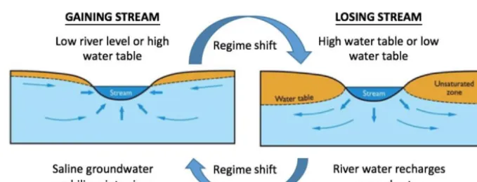
In order to apply the proposed approach, a suitable concep-tual understanding of the processes that affect salinity in the system under consideration is required. In general, a distinc-tion can be made between in-stream salt transport and the accession/addition of salt into the main channel via a variety of mechanisms that are affected by whether the river is oper-ating under normal or flood conditions (Tefler et al., 2012), as illustrated in Fig. 2. The transport of in-stream salt occurs along the main channel, from the top of the figure flowing through the river toward the bottom. Under normal condi-tions, the only potential source of salt accession is generally via the inflow of saline groundwater, provided the stream is gaining (i.e. if the height of the water table is above the river level) (Fig. 3). However, during these conditions, salt from the groundwater store can also mobilise into various floodplain elements, such as wetlands and anabranches. In addition, the salt load in these floodplain elements increases
as a result of evapo-concentration. Under flood conditions (Fig. 2), saline inflow from groundwater is likely to cease, as the river level is likely to be higher than the water table, resulting in a reversal of the flow direction (Fig. 3). Con-sequently, instead of the river gaining water (and salt) from groundwater, there will be a loss of fresh water from the river to recharge the groundwater system.
However, wetlands and anabranches that are disconnected under normal flow conditions may connect to the main river channel under flood conditions, adding salt that has been building up in these systems since the last flood when wa-ter levels recede. The amount of salt added is a function of the magnitude of the flood and the time and conditions (e.g. degree of evapo-concentration) since the occurrence of the last flood. Broader inundation of the floodplain results in recharge to the groundwater system, and leads to increased flux, and hence salt load, from the groundwater system to the river once the river level returns to normal conditions. As part of the proposed approach, all of the specific sub-processes that contribute to salinity for the case study under considera-tion need to be identified.
2.3 Identification of the most suitable model types As part of this step, the model types that are most suitable for modelling the relevant sub-processes identified in the pre-vious step are determined based on joint consideration of model purpose, system understanding and data availability and suitability (Fig. 1). Model purpose has an influence on which of the relevant processes have to be modelled explic-itly. For example, if the overall purpose of the modelling ex-ercise is to obtain salinity forecasts at downstream locations, there might not be a need to model all contributing processes explicitly (Maier and Dandy, 1996). In contrast, if the pur-pose of the model is to gain increased system understanding or to enable the impacts of various salt management options to be considered, all sub-processes will most likely have to be modelled explicitly. This also has an impact on which poten-tial model inputs are considered. For example, if forecasting is the primary model purpose, auto-regressive values of the model output should be considered as potential inputs (e.g. Bowden et al., 2005b), as this is likely to improve the qual-ity of the forecasts. In contrast, if the purpose of the model is to assess the impact of different management options on salinity, auto-regressive values of the model output cannot be considered as potential model inputs, as the model output has to be independent of the model input(s) in such cases.
trans-Figure 2.Processes affecting saline accessions during normal and flood conditions.
Figure 3.Processes affecting saline groundwater accessions for gaining and losing streams.
port of a conservative constituent with discharge, i.e. the pro-cess of in-stream salt transport, is generally well understood and requires relatively little data to be modelled explicitly, as the main processes consist of flow routing and storage. Con-sequently, the use of process models might be most appro-priate. However, the same is unlikely to be true when mod-elling different processes of salt accession, as these are gen-erally more complex, site specific (depending on soil types and groundwater conditions) and less well understood, mak-ing more hypothetically-influenced models an attractive al-ternative. If sufficient data are available, the use of univer-sal function approximators, such as artificial neural networks (ANNs), might be best (Mount et al., 2016). However, a scarcity of data representing rare events, such as the large flood events that might be required to flush the salt stores in the wetlands and anabranches adjacent to the main river channel, might make models with a smaller number of pa-rameters, such as regression, a better option.
It is important to note that the proposed framework is con-ceptual in nature and designed to provide high-level guid-ance. Consequently, its implementation for particular case studies is subjective. For example, how much data is required to support a particular modelling approach is case study
de-pendent and relies on the judgement of the model devel-oper. Consequently, this stage of the process may be iterative. Following the application of the developed sub-models, re-sults may assist in identifying limitations in understanding or missing information. Hence, understanding gained from the application of the sub-model combinations developed may be applied to optimise the number and type(s) of sub-models included in the final hybrid model.
2.4 Development of required sub-models and hybrid model
[image:5.612.127.467.270.400.2]Queensland
South Australia
New South Wales
Victoria Disher Creek
Pike River
Gurra Gurra lakes Lyrup forest flood connection
Lock 5
Lock 4
Murray River study reach
Berri irrigation extraction
1 km Study
reach
N
[image:6.612.129.466.64.376.2]Lyrup pumping station
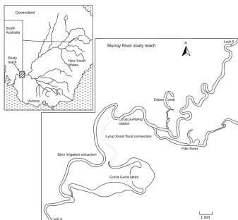
Figure 4.Map of case study reach.
3 Case study 3.1 Background
In order to illustrate and test the utility of the conceptual high-level framework introduced in Sect. 2, it is applied to a case study of the 46 km reach between Lock 5 and Lock 4 on the Murray River in South Australia (Fig. 4). This partic-ular location is chosen due to the following:
– The reach is underlain by highly saline regional ground-water systems that provide significant salt accession into the river along this reach. As such, there are sub-stantial saline accessions in this reach that are not well understood.
– This reach exemplifies a range of processes that are known to facilitate salt accession into a reach of a river, such as groundwater gain, inflow from streams, creeks and wetlands, and in-channel transport.
– Conditions along this reach have been monitored for many years, so there are suitable datasets for model de-velopment.
– The reach has had minimal changes in salinity manage-ment over time, so external influences on the underlying
processes represented by the historical data are mini-mal.
– A number of changes are occurring in the Murray River system that will result in changes in the flow and inun-dation regime:
a. The Murray–Darling Basin Plan, as per parts 1A and 2 of the Commonwealth Water Act (2007), will return some water previously allocated to consump-tive use to the environment, with the aim of in-creasing ecosystem health through processes such as increased frequency of inundation. The ability to predict the effects on salinity resulting from these changes is currently very limited.
3.2 Identification of relevant sub-processes
The main processes affecting salinity in the reach of inter-est include in-channel salt transport, as well as accession of salt via groundwater and flushing of several large floodplains and wetlands. There are also several anabranches and back-waters, which include Pike River, the Gurra Gurra lakes and Disher Creek (Fig. 4). In-channel salt transport is primarily driven by advection with flow in the main river channel, as well as the storage mixing volume behind the lock, which may change as water levels are manipulated.
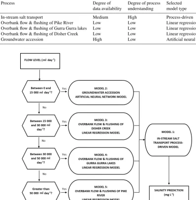
Saline accession via groundwater is a function of the rel-ative levels of the groundwater adjacent to the river chan-nel and the water levels in the main river chanchan-nel. As dis-cussed in Sect. 2.2, if the water levels in the main river chan-nel are below the adjacent groundwater levels, groundwater flows into the main river. As the salinity of the groundwater that flows into the main river channel in the reach of inter-est is very high (up to 70 000 mg L−1)(Barnett, 2007), this can be a significant source of saline accession. Analysis of the available data from groundwater wells (WaterConnect, 2016) showed that groundwater levels are relatively constant and that saline groundwater accession occurs at flows below approximately 40 000 ML day−1, after which overbank flow commences. This is useful in that it demonstrates a link be-tween groundwater accession and river flow rate, and implies that models of such processes are unhelpful at higher flows.
There are three large salt sources that connect to the river at different flow rates: Disher Creek, Gurra Gurra lakes and the Pike River. Disher Creek is an evaporation basin for ir-rigation runoff and salt interception scheme flows. Water is held in the basin to be disposed of through evaporation or, if this is not sufficient, water can be pumped to the Noora drainage disposal basin 20 km away from the river. The man-agement rules for Disher Creek allow for the release of water from the evaporation basin to the river at flows greater than 15 000 ML day−1, which is assumed to be sufficient to di-lute the highly saline releases from the basin. It should be noted that releases are not always triggered at this flow, and the release rate can be modified depending on the measured salinity in the river at the time.
At lower river flows, the Gurra Gurra lakes are a termi-nal wetland system, with one connection to the river. Under these conditions, evaporation removes water from the wet-land, which is then replaced from the river, and this pro-cess results in naturally higher salinities than in the main river channel. At flows of approximately 30 000 ML day−1
the water level in the river rises high enough to connect the flow path to the north of the lakes (through Lyrup Forest), resulting in a through-flowing system. When this is the case, the lakes are flushed, and the saline water from the wetlands contributes to the main river channel, thus increasing its salt content.
The Pike River is an anabranch that loops around Lock 5 and the upper area of the reach. The lock provides a 3 m head
difference, and due to this, the Pike River can flow around the lock and back into the river below it. There are two inlets to the Pike River above Lock 5, which are both regulated; this was historically to supply flows for irrigation purposes. At flows approaching 50 000 ML day−1, the main river chan-nel begins to overflow, and connects a number of temporary flow paths to the Pike River, resulting in wash-off and trans-port of salt that may have been deposited on the floodplain in that locality. This flow of 50 000 ML day−1is representa-tive of when overbank flows start to occur along the reach between locks 4 and 5 (and the lower Murray River more broadly), where this process occurs along the river, as well as the longer-term process of recharge to groundwater and increased flux once river levels recede.
It should be noted that the amount of salt flushed into the main river channel from these systems is difficult to predict, as it is not only a function of flow, but also of the time be-tween flushing events, the duration of an event and the na-ture of the flow regime at the time. Moreover, the accession processes are very different at different flow regimes. For ex-ample, at 15 000 ML day−1, the salt contribution from Disher Creek may be represented by a point load into the main chan-nel. However, at flows greater than 40 000 ML day−1, Disher Creek disappears entirely from the map, as it is swallowed by an extensive floodplain. When this occurs, the creek does not contribute any additional salt to the system: it has already been entirely flushed and the only water in the area is flowing downstream as part of the flooded main river channel. 3.3 Identification of relevant sub-models
The purpose of the hybrid model is to quantify salinity re-sponses to proposed managerial changes to the flow and in-undation regime in the reach of the river under consideration under the Murray–Darling Basin Plan. These changes will be enacted by the construction of additional control struc-tures, and by selective releases or routing of volumetric flow. The salinity response to such changes is of interest in that the consequences of poor water quality can be high, and the modelling of different processes of accession is poorly understood. There is consequently value in identifying and modelling the main processes of accession separately, so that future management may determine the best locations of con-trol options in addition to assessing the magnitude of their effects on salinity.
instru-Table 1.Details of available model data. All data are recorded at a daily resolution and have been sourced from DEW (Department of Environment, Water and Natural Resources).
Parameter Location (Station Number) Time Period
Flow rate (ML day−1) Lock 5 (downstream, A4260513) 23 Jan 1981–25 May 2016 Flow rate (ML day−1) Lock 4 (downstream, A260515) 1 Jul 1983–30 Jun 2012 Flow rate (ML day−1) Lyrup pumping station (A4260663) 12 Nov 1993–18 Jun 2017 Temperature (◦C) Berri irrigation extraction (A4260537) 29 Mar 2001–2 Aug 2016 Temperature (◦C) Pike River outlet (downstream, A260645) 26 Sep 1991–18 Jun 2017 Salinity (mg−1) Lock 5 (upstream, A4260512) 4 Jul 1972–1 May 2013 Salinity (mg L−1) Lock 4 (upstream, A1260514) 18 Jan 1994–20 Mar 2017 Salinity (mg L−1) Pike River outlet (downstream, A260645) 26 Sep 1991–18 Jun 2017 Salinity (mg L−1) Berri irrigation extraction (A4260537) 17 Oct 1942–20 Mar 2017 Water level (m) Lock 5 (downstream, A4260513) 1 Apr 1924–1 May 2013 Water level (m) Lyrup pumping station (A4260663) 11 Nov 1993–18 Jun 2017 Water level (m) Lock 4 (upstream, A1260514) 1 Apr 1927–1 May 2013 Water level (m) Berri irrigation extraction (A4260537) 1 Jan 1974–20 Mar 2017 Salt load (kg day−1) Lock 4 (downstream, A260515) 1 Jul 1983–30 Jun 2012
ments to measure certain parameters were commissioned. Some datasets are deemed not suitable for model develop-ment and are therefore excluded from this study, often due to short data records of only a few years in length (e.g. mea-surements taken at the mouth of Gurra Gurra lakes). Key lo-cations include the two locks that define the extent of the reach considered, as well as the Pike River anabranch. Berri river extraction and Lyrup pumping station, which are down-stream of the Pike River, also provide useful information for salt transport and accession along the reach.
As discussed in Sect. 2.3, which modelling approach is most suitable for a particular process is a combination of the degree of process understanding and data availability. The relative degree with which these two factors are satisfied for the processes to be modelled in this case study (see Sect. 3.2), based on a subjective assessment of available information, is summarised in Table 2. As can be seen, the processes affect-ing in-stream salt transport are well understood, able to be represented mathematically and supported by sufficient data to enable a process-driven model to be developed. However, the processes associated with the various modes of saline ac-cession are not considered to be well understood, making data-driven models the best option. In relation to ground-water accession, the degree of available data is high, as this occurs during non-flood events and relevant data are mea-sured daily. Consequently, an artificial neural network is con-sidered the most appropriate modelling approach due to its universal function approximation ability and its successful application to the prediction of salinity in the Murray River in previous studies (e.g. Maier and Dandy, 1996). However, as the saline accessions corresponding to overbank flow and flushing only occur during flood events, which occur infre-quently, the data available on these processes is considered insufficient to support the development of a model with a potentially large number of parameters, such as an artificial
neural network. Instead, a linear regression model is consid-ered most appropriate to represent these processes due to the combination of a low degree of process understanding and a low degree of data availability.
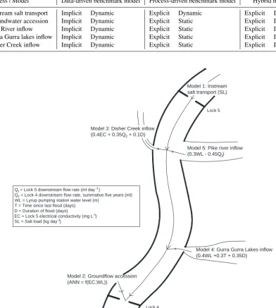
A conceptual representation of the resulting hybrid model is given in Fig. 5. As can be seen, the models corresponding to the four main sub-processes associated with saline acces-sion identified in Sect. 3.2 are conceptualised as being appli-cable at different flow rates. This was determined based on a preliminary analysis of the available data, with one model being applied to only one discrete bracket of flow. As a re-sult, while each model primarily represents the process with which it is associated, it might also represent other processes that occur during the range of flows for which each model is developed. As shown in Fig. 5, the four models of saline ac-cession (models 2 to 5) feed into the in-stream salt transport model (model 1).
3.4 Development of required sub-models and hybrid model
In this section, details of the development of the five sub-models (Fig. 5) are given. The modelling data and perfor-mance metrics are described first, as they are common to all models, followed by details on the development of the three different modelling types (i.e. process-driven (model 1), arti-ficial neural network (model 2) and linear regression (models 3 to 5)). This is followed by details of the model development process for each of these model types, as well as how they are combined to form the hybrid model.
3.4.1 Model development data
[image:8.612.117.478.96.279.2]Table 2.Identified processes and the degree of data and understanding that are available for each.
Process Degree of Degree of process Selected
data availability understanding model type
In-stream salt transport Medium High Process-driven
Overbank flow & flushing of Pike River Low Low Linear regression Overbank flow & flushing of Gurra Gurra lakes Low Low Linear regression Overbank flow & flushing of Disher Creek Low Low Linear regression
Groundwater accession High Low Artificial neural network
Figure 5.Conceptual representation of components of hybrid model and how they are connected.
data (1–3 days) are filled in using linear interpolation, which is common practice for gaps in data of this duration and is unlikely to result in any significant loss of information (Ko-rnelson and Coulibaly, 2014). Two longer periods of miss-ing flow data at Lock 5 in the period 2011–2012 (132 and 72 days, respectively) are filled in by correlation with cor-responding water level data. To ensure consistency between sub-models, the longest common period of available data is used for the development of all models, which is from 18 January 1994 to 30 June 2012. The available data are split so that the first 80 % (i.e. from 18 January 1994 to 21 Octo-ber 2008) are used for model calibration and the subsequent 20 % (i.e. from 22 October 2008 to 30 June 2012) are used for validation for all models. It should be noted that a re-gional drought event from 2001 to 2010, which is reflected
in almost a decade of low flows (< 15 000 ML day−1), is the most significant unusual feature in the data and is purposely split between both calibration and validation datasets. To en-sure all inputs into the ANN and regression models span the same ranges and can thus be combined during the modelling process, all data are standardised to have a mean of zero and a standard deviation of one, as per Eq. (1).
y=(x− ¯x)
σ , (1)
[image:9.612.90.489.90.497.2]3.4.2 Model performance assessment
All data are calibrated and validated against the salinity at Lock 4. The root mean squared error (RMSE, Eq. 2) and the Nash–Sutcliffe Efficiency (NSE, Eq. 3) are used as metrics to judge the fit of the predicted variables to the observed data when calibrating the parameters of the models:
RMSE= v u u t 1 n n X
i=1
xmi −xoi 2
(2)
NSE=1−
n
P
i=1
xmi −xoi2
n
P
i=1 xi
o− ¯xo2
, (3)
wherenis the number of points in the series,xmis modelled
points,xois observed points andx¯ois the mean of observed
points.
The goodness of fit of the hybrid model is evaluated against two benchmark models, one process-driven and one data-driven, with the metric Gbench introduced in
Seib-ert (2001) (Eq. 4):
Gbench=1− n
P
i=1
xoi−xmi 2
n
P
i=1 xi
o−xib 2
, (4)
wherexbare the benchmark model data points.
TheGbenchindex is structured similar to the NSE, but
re-places the mean of the observed time series with the time series of a benchmark model: therefore an index of zero in-dicates that model performance is equal to that of the bench-mark model, negative values indicate that the performance of the model under consideration is inferior to that of the bench-mark model and positive values indicate the opposite. 3.4.3 Process-driven salt transport sub-model
(model 1)
The purpose of this model is to simulate the in-stream trans-port of salt from Lock 5 to Lock 4, thereby predicting salinity at Lock 4 as a function of the upstream salt load, without con-sidering saline accessions due to groundwater inflow or the flushing of anabranches and backwaters along the reach. The model is developed using eWater Source (Welsh et al., 2013). Routing is represented using a piecewise linear lookup table, where the travel times for key flow rates are calculated based on travel times of flow peaks in the historical record. A dead storage volume is used to represent the mixing time for salin-ity, as the travel time for solutes is much slower than the wave celerity travel time resulting from the analysis of flow peaks. The routing or transportation method is a fully mixed water quality constituent. This technique has been used since the
1970s in various water quality models and hence is well de-veloped. The key principles are that the mass balance of the modelled constituents (e.g. salt) is maintained in all divisions of all links (which represent a reach). Calculations take place for every time step, which is daily.
Development of the travel times and dead storage volumes for all areas of the river were calibrated in a previous study, as outlined in MDBC (2002). The salt constituent volumes in the upstream reaches were also determined as part of this previous work, however, the salt accession within the study reach itself is considered as part of the calibration process. As this is a process-driven model, the required inputs are predetermined due to the mathematical specification of the model. These include upstream flow and salinity at Lock 5, and knowledge of the physical characteristics of the reach, such as its total length and the location of various extrac-tion points (e.g. Lyrup pumping staextrac-tion and Berri irrigaextrac-tion extraction). The transport model routes the upstream salt through the reach down to Lock 4, and converts it into salin-ity by multiplying the salt load with the rate of flow. The dif-ference between this transported salinity and the measured salinity at Lock 4 (i.e. the residual salinity of model 1) repre-sents the salt that is gained by the river due to the accession processes that occur within the reach itself (Sect. 3.2), and is the salinity that is predicted by the remaining hybrid compo-nent models (i.e. models 2, 3, 4 & 5).
3.4.4 Artificial neural network (ANN) groundwater accession model (model 2)
The purpose of this model is to predict accession of salt for flows that are less than 15 000 ML day−1, which is sourced
primarily from groundwater inflows and small increases in water level at the upstream end of the reach between locks 5 and 4. These tend to occur due to the same mechanisms along large stretches of the river during a single dry or wet event. However, their response times can be vastly different, ranging from days for responses to changing water levels, to months for the slower responses to saline groundwater acces-sions.
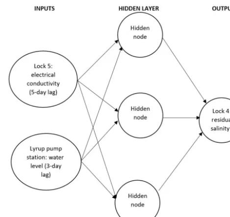
deter-mined with the aid of correlation analyses between potential model inputs and the model output, resulting in the selec-tion of two inputs: (1) salinity at Lock 5, and (2) the water level measured at Lyrup pumping station (Fig. 6), which are lagged by 5 and 3 days, respectively. The selected inputs re-flect that saline accessions at low flows are primarily driven by upstream salinities (primarily affecting water level) and water levels (primarily affecting groundwater inflow).
Multilayer perceptrons (MLPs) are used as the model ar-chitecture, as this is by far the most commonly used architec-ture in ANN applications in hydrology and water resources (Maier et al., 2010; Wu et al., 2014). Different combinations of standard activation functions (linear, sigmoidal and hyper-bolic tangent) are trialled on the calibration data, resulting in the selection of the hyperbolic tangent function applied to the single hidden layer and the linear function being ap-plied to the output layer. An ANN with three hidden nodes performs best on the calibration data, based on trials with one to four hidden nodes. The ANN is fully connected, so there are nine weighted connections (i.e. nine parameters to calibrate). The development data contain 5391 points (i.e. 5391 days over the calibration period), so there are almost 600 data points available to calibrate each parameter, making overfitting unlikely. These parameters are calibrated using the Broyden–Fletcher–Goldfarb–Shanno (BFGS) algorithm, as this method generally performs well when simulating hy-drological phenomena (Zounemat-Kermani et al., 2016). Op-timal values of the learning rate and momentum are obtained using trial and error on the calibration dataset, and the ini-tial weights are selected randomly on the range [−0.5,0.5]. To test against overfitting, the model is validated against the residual salinity between the transport model (model 1) and the measured salinity at Lock 4, over the period 22 October 2008 to 30 June 2012 for all data points corresponding to flow rates at Lock 5 of less than 15 000 ML day−1.
3.4.5 Linear regression models for Disher Creek, Pike River and Gurra Gurra lakes accession (models 3 to 5)
The purpose of the linear regression models (models 3 to 5, Fig. 5) is to predict accessions of salt to the river at flows in excess of 15 000 ML day−1. These flows are dominated by Disher Creek and Pike River at a point downstream from Lock 5 (see Fig. 4), and the inflow from the Gurra Gurra lakes at a point upstream from Lock 4 (Fig. 4); they are also likely to include saline accessions from groundwater and increases in water level at flows closer to 15 000 ML day−1. The data in
[image:11.612.311.546.64.285.2]Table 1 are available as potential inputs for model develop-ment, with the most relevant inputs determined by trial and error during the calibration process. Because of the scarcity of peak flow data and the complexity of the physical pro-cesses being modelled, it is valuable to incorporate as much process understanding into these models as possible. This is achieved by ensuring that some of the more important known
Figure 6.Structure and inputs of ANN model for predicting saline groundwater accession as part of the hybrid model (model 2). The residual salinity output is the difference between the measured salinity and the output from the process-driven salt transport model for all flow rates that are less than 15 000 ML day−1.
process drivers, such as peak duration, time since last peak flow and historical flow volumes, are represented as poten-tial model inputs, as follows:
– The 5-year historical volume of water (ML) is extracted from the daily flow rate measurements at Lock 5 (Q2)
because residual waters from receding historical peaks or overbank flows can create concentrated pockets of salt once the water has evaporated, which is then avail-able to be accessed by the next overbank flow.
– The duration of the peak flow event (D) is extracted as a count of days, which begins incrementing at the com-mencement of a peak flow event. This is due to the fact that longer floods allow the extended floodplain more time to connect with groundwater aquifers at a distance from the river, and to react with the salt content of the soil.
– The time since last peak flow (T) is extracted as a count of days, which begins incrementing when the daily flow rate falls below the defined peak flow. This is because a longer time since the last peak allows for a greater amount of saline groundwater to seep into depressions and shallow reservoirs, which may be some distance from the main channel, thereby increasing the amount of salt available for overbank flow.
of an individual model. For example, a peak flow event for model 3 is any daily flow that is 15 000 ML day−1or higher,
while a peak flow event for model 5 is any daily flow that is 50 000 ML day−1or higher.
The models are developed in Microsoft Excel, using the Solver function (i.e. a gradient method) to optimise the coef-ficients from a range of starting positions and to minimise the chance of identifying locally optimal parameter values. The models are calibrated against the residual salinity at Lock 4 obtained from the process-driven in-stream salt transport model (model 1), over the time period from 18 January 1994 to 21 October 2008, using the NSE as the objective function. Data from 22 October 2008 to 30 June 2012 are used for val-idation, however, flow data from 18 January 1989 are also used in order to calculate the summed, volumetric flow from 5 years previous (Q2), which is considered as a potential
in-put for these models, as mentioned above.
The resulting equations for models 3, 4, and 5 are given by Eqs. (5), (6) and (7), respectively:
model 3
RSp=0.4EC+0.35Q2+0.1D if 15 000≤Q1<30 000;
(5) model 4
RSp=0.4WL+0.3T +0.35D if 30 000≤Q1<50 000;
(6) model 5
RSp=0.3WL−0.45Q1 if Q1>50 000, (7)
where RSp are the residuals between the measured salinity
and the output salinity from the process-driven salt trans-port model for all peak flow rates greater than or equal to 15 000 ML day−1(mg L−1);Q1is the flow rate downstream
of Lock 5 (ML day−1);Q2is the 5-year historical volume of
water at Lock 5 (ML); WL is the water level at Lyrup pump station (m);T is the time since last peak flow (days);D is the duration of peak flow event (days); and EC is the salinity downstream from Lock 5 (mg L−1).
The selected inputs for model 3 indicate a positive cor-relation with salinity at Lock 5 (EC), the 5-year historical flow volume at Lock 5 (Q2)and peak flow event duration
(D). The positive correlation with EC is most likely related to shallow overbank flow, as discussed in Sect. 3.5.4.Q2is
likely to increase salt load, as greater volumes of historical flow indicate a greater likelihood that events that generate saline accessions have occurred in the previous 5 years. Fur-thermore,Dis likely to be positively correlated with saline accessions, as longer flood durations provide more time for groundwater recharge during an event and therefore later discharge on the recession of a flood, which in turn results in slow response saline accessions.
The selected inputs for model 4 indicate a positive corre-lation with higher water levels at Lyrup pump station (WL), time since last peak flow (T) and peak flow event duration (D). The positive correlation with WL is most likely due to the fact Lyrup pump station is just upstream of the connec-tion that flushes Gurra Gurra lakes at high flows, with higher water levels at Lyrup pump station providing an indication of an increased ability to flush the lakes. Higher values of time since last peak flow are likely to increase saline accessions, as longer periods of time between floods provide more time for evapo-concentration to occur, as well as saline groundwa-ter to flow into the Gurra Gurra lakes system, which is very shallow. Finally, as is the case for model 3, longer flood dura-tions provide more time for stored saline water to be flushed into the main river channel.
The selected inputs for model 5 indicate a positive corre-lation with higher water levels at Lyrup pump station (WL) and a negative correlation with flow downstream of Lock 5 (Q1). The positive correlation with WL is most likely related
to the fact that larger areas of the floodplain are inundated at higher water levels, increasing overall salt load. The negative correlation with flow is most likely due to the increased di-lution of the salt load at the high flows to which this model caters.
3.4.6 Hybrid model
A schematic of the resulting hybrid model is shown in Fig. 7. As can be seen, the process-driven in-stream salt trans-port model (model 1) forms the basis of the hybrid model, with the different types of accessions, modelled using the ANN and regression models, added at appropriate locations. Specifically, the first and second regression models (models 3 and 4, respectively) are added downstream of Lock 5, at the approximate location of the Pike River and Disher Creek out-lets. The third regression model (model 5) is added upstream of Lock 4, near the entrance of Gurra Gurra lakes. The output from the groundwater accession ANN (model 2) is added to model 1 at Lock 4. Although groundwater accession occurs along the length of the reach under consideration, these in-flows are impractical to segregate. The outputs from models 2 to 5 are only added to model 1 when triggered by the cor-responding flow rate in a given time step: there is only one model besides model 1 that describes the salinity levels on any given day.
3.5 Development of benchmark models
Table 3.Method by which different processes are represented by the hybrid and benchmark data- and process-driven models. The inputs are represented either explicitly (by separate processes within the model) or implicitly. The outputs are either dynamic (the salt load varies in response to some time-dependent environmental changes) or static.
Process | Model Data-driven benchmark model Process-driven benchmark model Hybrid model
In-stream salt transport Implicit Dynamic Explicit Dynamic Explicit Dynamic Groundwater accession Implicit Dynamic Explicit Static Explicit Dynamic
Pike River inflow Implicit Dynamic Explicit Static Explicit Dynamic
Gurra Gurra lakes inflow Implicit Dynamic Explicit Static Explicit Dynamic
Disher Creek inflow Implicit Dynamic Explicit Static Explicit Dynamic
Model 1: Instream salt transport (SL)
Model 5: Pike river inflow (0.3WL - 0.45Q1)
Model 3: Disher Creek inflow (0.4EC + 0.35Q2 + 0.1D)
Model 4: Gurra Gurra Lakes inflow (0.4WL +0.3T + 0.35D)
Model 2: Groundflow accession (ANN = f(EC,WL))
Lock 4
Lock 5
Q = Lock 5 downstream flow rate (ml day )1 -1
Q = Lock 4 downstream flow rate, summative five years (ml)2
WL = Lyrup pumping station water level (m) T = Time since last flood (days) D = Duration of flood (days)
EC = Lock 5 electrical conductivity (mg L-1)
SL = Salt load (kg day )-1
Figure 7.Schematic of the hybrid model on a stylised view of the river (not to scale). The regression models are input as point loads, while the groundwater accession is added to the transport model at Lock 4.
of interest explicitly, this is done via the addition of average historical accessions, as this represents the best available in-formation. Consequently, unlike the hybrid model, which ac-counts for saline accession in a dynamic fashion, the bench-mark process-driven model does so in static fashion. How-ever, in-stream salt transport processes are represented in an explicit and dynamic manner. In contrast, in the benchmark ANN model, all processes are represented implicitly, as it predicts salinity at Lock 4 as a function of available data
[image:13.612.103.496.118.555.2]de-Table 4.Performance statistics for the hybrid model and its component models for the validation data.
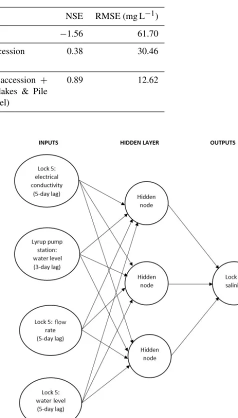
Model NSE RMSE (mg L−1)
In-stream salt transport (model 1) −1.56 61.70
In-stream salt transport+groundwater accession (models 1+2)
0.38 30.46
In-stream salt transport + groundwater accession + flushing of Disher Creek, Gurra Gurra lakes & Pile River (models 1–5 – complete hybrid model)
0.89 12.62
tails of the development of the two benchmark models are given in the subsequent sections.
3.5.1 ANN model (benchmark)
The purpose of this ANN model is to predict the total salinity in the river at Lock 4 directly. This is in contrast to the ANN model that forms part of the hybrid model (model 2), which predicts the residual salinity between the process-driven in-stream salt transport model predictions and the measured salinity at Lock 4 for flows up to 15 000 ML day−1. The latter
is aimed at representing groundwater accession and low flow processes only. As mentioned above, the benchmark ANN model is developed using the same methodology as that used for model 2 (see Sect. 3.5.4). A summary of the resulting ANN model is given in Fig. 8.
3.5.2 Process-driven model (benchmark)
The benchmark process-driven model is identical to the one used in the hybrid model. However, as shown in Table 3 and described above, while salt accession within the study reach is modelled dynamically using ANN and regression models in the hybrid model, in the benchmark model salt accession is represented as an average of historical salt loads. This is done by calculating the average daily salt load at Lock 4 for the calibration period of 18 January 1994 to 21 Octo-ber 2008, which is then applied as two constant point loads. Most (approximately 82 %) of this load is applied upstream of the Berri irrigation extraction, as this area forms a longer part of the study reach than the area downstream of this loca-tion. The remainder of the constant salt load is applied down-stream from Berri.
4 Results and discussion
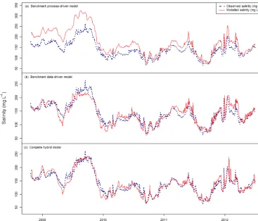
The time series plots of actual versus predicted salinities for the hybrid model and its component models for the valida-tion data are given in Fig. 9, with the corresponding perfor-mance statistics given in Table 4. As can be seen, the hybrid model performs very well, with a NSE of 0.89 and an RMSE of 12.62 mg L−1(for data ranging from approximately 50 to 250 mg L−1). The time series plot shows that the model has
Figure 8.Structure and inputs of the benchmark ANN.
captured all variations in salinity very well, with only small over- or under-predictions (Fig. 9c).
[image:14.612.305.543.81.499.2]Figure 9.Measured versus modelled salinity at Lock 4 for the hybrid model and its components for the validation data, as well as corre-sponding hydrograph for Lock 5.
lakes and Pike River (models 3 to 5) are added, an NSE value of 0.89 and an RMSE value of 12.62 mg L−1are achieved as a result of increased performance during high flow periods. This indicates the value of the proposed hybrid approach, as each of the models of the different sub-processes improve model performance significantly.
The hybrid model also performs favourably compared with the two benchmark models, as shown in Table 5 and Fig. 10. The process-driven benchmark model performs sig-nificantly worse than the hybrid model, with NSE and RMSE values of −0.14 and 41.10 mg L−1, respectively, compared with corresponding values of 0.89 and 12.62 mg L−1for the hybrid model. As can be seen in Fig. 10, this is due to an over-prediction of saline accessions by the benchmark process-driven model, as these are based on static historical values rather than being modelled dynamically as a function of changes in flow, water levels and upstream salinity, as is the case for the hybrid model. However, the addition of the average values of the historical saline accessions results in an improvement in model performance compared with that of the process-driven in-stream salt transport model used in the hybrid model (model 1) – an increase in NSE from−1.56 to
−0.14 and a reduction in RMSE from 61.70 to 41.10 mg L−1.
In contrast to the process-driven benchmark model, the data-driven benchmark model performs only slightly worse than the hybrid model, with NSE and RMSE values of 0.83 and 15.93 mg L−1, respectively, compared with correspond-ing values of 0.89 and 13.58 mg L−1 for the hybrid model. As can be seen in Fig. 10, the primary differences between the hybrid and data-driven benchmark models are that the benchmark model under-predicts saline accessions during low-flow periods (e.g. towards the end of 2009) and over-predicts saline accessions during high-flow periods (e.g. in the first half of 2011 and 2012). This highlights the benefits of the hybrid model in being able to tailor models to acces-sions during low- and high-flow periods. The superior perfor-mance of the hybrid model is reinforced by positive values of theGbenchindex of 0.36 and 0.90 for the data-driven and
process-driven benchmark models, respectively.
Figure 10.Measured versus modelled salinity at Lock 4 for the hybrid model and the two benchmark models for the validation data.
Table 5.Performance statistics for the two benchmark models and the hybrid model for the validation data.
Model NSE RMSE (mg L−1)
Process-driven benchmark model −0.14 41.10 Data-driven benchmark model 0.83 15.93
Hybrid model 0.89 13.58
river management is being expanded to include the improve-ment of environimprove-mental outcomes. This includes changing the flow regime via the delivery of environmental water, and by constructing control infrastructure on the floodplain to in-crease inundation frequency and duration. As the variables that affect the flow regime are included as inputs in the hy-brid model, this model can be used to assess the impact of some of the proposed management options on river salinity. In addition, the hybrid model contributes to an increased un-derstanding of the underlying processes.
Overall, the results of the illustrative case study highlight the potential benefits of the proposed framework. By con-sidering the relevant processes affecting river salinity at the site of interest, how well they are understood and can be represented mathematically, how much data there is to
sup-port model development and what the primary purpose of the model is, a hybrid model was able to be developed that not only results in better predictive performance than the cor-responding benchmark process- and data-driven models, but is also more useful from a management perspective. How-ever, given the conceptual nature of the proposed framework and the level of subjectivity required to implement it, it is not possible to tell if an even better model could have been developed had different decisions been made with regard to model types.
5 Summary and conclusions
This paper introduces a framework for the development of hybrid models for the prediction of salinity in rivers. As part of the framework, relevant sub-processes contributing to river salinity are identified, followed by the selection and development of the most appropriate sub-models for each of these based on model purpose, degree of process understand-ing and data availability, which are then combined to form the hybrid model.
[image:16.612.46.287.456.515.2]model, an ANN model to primarily cater to saline ground-water accessions and three linear regression models to ac-count for the flushing of three different waterbodies in the floodplain. Results show that the hybrid model performs very well and is able to capture all variations in salinity with high levels of accuracy. The value of using a hybrid approach is demonstrated by the incremental increase in model perfor-mance when different sub-models are added. The superior performance of the hybrid model compared with that of two benchmark models, based on commonly used methods for modelling salinity in rivers including a process-driven and a data-driven ANN model, further highlights the model’s value. In addition to superior predictive performance, the hy-brid model results in the development of increased process understanding and is able to be used to assist with the evalu-ation of various river management options.
Overall, the proposed hybrid approach shows significant promise, although there would be value in applying it to dif-ferent river systems where difdif-ferent processes dominate and different types of data are available. While the approach has been developed specifically for the modelling of salinity in rivers, there is no reason why some of the underlying princi-ples cannot be applied successfully for other types of hydro-logical models.
Data availability. All sets of original data used in the production of
this paper are available publicly from the Surface Water Data Sys-tem repository at https://www.waterconnect.sa.gov.au (last access: 9 November 2017). Readers and reviewers are encouraged to con-tact the corresponding author directly for any extracted sets of data (salt load, peak flow duration, etc.).
The Supplement related to this article is available online at https://doi.org/10.5194/hess-22-2987-2018-supplement.
Competing interests. The authors declare that they have no conflict
of interest.
Acknowledgements. The authors would like to thank the two
anonymous reviewers for their comments, which improved and clarified the manuscript.
Edited by: Dimitri Solomatine Reviewed by: two anonymous referees
References
Adamowski, J. and Chan, H. F.: A wavelet neural network conjunc-tion model for groundwater level forecasting, J. Hydrol, 407, 28– 40, https://doi.org/10.1016/j.jhydrol.2011.06.013, 2011. Alvarez-Garreton, C., Ryu, D., Western, A. W., Su, C.-H., Crow,
W. T., Robertson, D. E., and Leahy, C.: Improving opera-tional flood ensemble prediction by the assimilation of satel-lite soil moisture: comparison between lumped and semi-distributed schemes, Hydrol. Earth Syst. Sci., 19, 1659–1676, https://doi.org/10.5194/hess-19-1659-2015, 2015.
Banerjee, P., Singh, V. S., Chatttopadhyay, K., Chandra, P. C., and Singh, B.: Artificial neural network model as a potential alterna-tive for groundwater salinity forecasting, J. Hydrol., 398, 212– 220, https://doi.org/10.1016/j.jhydrol.2010.12.016, 2011. Barnett, S.: Gurra Gurra Wetland Complex – Groundwater Data
Review, Dept. of Water, Land and Biodiversity Conservation, 4, 2007.
Beecham, R., Arranz, P., Boddy, J., Burrell, M., Gilmore, R., Javam, A., Martin, J., O’Neill, R., and Salbe, I.: Implementing daily salinity models in the NSW Murray Darling Basin tributaries, in: Modsim 2003, International Congress on Modelling and Sim-ulation, Vol 1–4: Vol 1: Natural Systems, Pt 1; Vol 2: Natural Systems, Pt 2; Vol 3: Socio-Economic Systems; Vol 4: General Systems, 362–367, 2003.
Bowden, G. J., Maier, H. R., and Dandy, G. C.: Opti-mal division of data for neural network models in wa-ter resources applications, Wawa-ter Resour. Res., 38, 1010, https://doi.org/10.1029/2001wr000266, 2002.
Bowden, G. J., Maier, H. R., and Dandy, G. C.: Input determina-tion for neural network models in water resources applicadetermina-tions. Part 1. Background and methodology, J. Hydrol., 301, 75–92, https://doi.org/10.1016/j.jhydrol.2004.06.021, 2005a.
Bowden, G. J., Maier, H. R., and Dandy, G. C.: Input determination for neural network models in water resources applications. Part 2. Case study: forecasting salinity in a river, J. Hydrol., 301, 93– 107, https://doi.org/10.1016/j.jhydrol.2004.06.020, 2005b. Bowden, G. J., Maier, H. R., and Dandy, G. C.: Real-time
de-ployment of artificial neural network forecasting models: Un-derstanding the range of applicability, Water Resour. Res., 48, W10549, https://doi.org/10.1029/2012WR011984, 2012. Chang, F.-J. and Chang, Y.-T.: Adaptive neuro-fuzzy inference
sys-tem for prediction of water level in reservoir, Adv. Water Re-sour., 29, 1–10, https://doi.org/10.1016/j.advwatres.2005.04.015, 2006.
Chang, F.-J. and Tsai, M.-J.: A nonlinear spatio-temporal lump-ing of radar rainfall for modellump-ing multi-step-ahead inflow fore-casts by data-driven techniques, J. Hydrol., 535, 228–236, https://doi.org/10.1016/j.jhydrol.2016.01.056, 2016.
Chang, F.-J., Tsai, W.-P., Chen, H.-K., Yam, R. S.-W., and Herricks, E. E.: A self-organizing radial basis network for estimating riverine fish diversity, J. Hydrol., 476, 280–289, https://doi.org/10.1016/j.jhydrol.2012.10.038, 2013.
Chang, F.-J., Chen, P.-A., Chang, L.-C., and Tsai, Y.-H.: Estimat-ing spatio-temporal dynamics of stream total phosphate concen-tration by soft computing techniques, Sci. Total Environ., 562, 256–269, https://doi.org/10.1016/j.scitotenv.2016.03.219, 2016. Clark, M. P., Kavetski, D., and Fenicia, F.: Pursuing the
hydro-logical modeling, Water Resour. Res., 47, W09301, https://doi.org/10.1029/2010WR009827, 2011.
Commonwealth of Australia: Water Act (An act to make provision for the management of the water resources of the Murray-Darling Basin, and to make provision for other matters of national inter-est in relation to water and water information, and for related pur-poses), Commonwealth Consolidated Acts, Sects. 28–32, 2007. Corzo, G. and Solomatine, D.: Baseflow separation
tech-niques for modular artificial neural network mod-elling in flow forecasting, Hydrol. Sci. J., 52, 491–507, https://doi.org/10.1623/hysj.52.3.491, 2007.
Corzo, G. A., Solomatine, D. P., Hidayat, de Wit, M., Werner, M., Uhlenbrook, S., and Price, R. K.: Combining semi-distributed process-based and data-driven models in flow simulation: a case study of the Meuse river basin, Hydrol. Earth Syst. Sci., 13, 1619–1634, https://doi.org/10.5194/hess-13-1619-2009, 2009. Dessie, M., Verhoest, N. E. C., Pauwels, V. R. N., Admasu, T.,
Poe-sen, J., Adgo, E., Deckers, J., and NysPoe-sen, J.: Analyzing runoff processes through conceptual hydrological modeling in the Up-per Blue Nile Basin, Ethiopia, Hydrol. Earth Syst. Sci., 18, 5149– 5167, https://doi.org/10.5194/hess-18-5149-2014, 2014. Duan, W. L., He, B., Takara, K., Luo, P. P., Nover, D., and Hu,
M. C.: Modeling suspended sediment sources and transport in the Ishikari River basin, Japan, using SPARROW, Hydrol. Earth Syst. Sci., 19, 1293–1306, https://doi.org/10.5194/hess-19-1293-2015, 2015.
Duku, C., Rathjens, H., Zwart, S. J., and Hein, L.: Towards ecosys-tem accounting: a comprehensive approach to modelling multi-ple hydrological ecosystem services, Hydrol. Earth Syst. Sci., 19, 4377–4396, https://doi.org/10.5194/hess-19-4377-2015, 2015. Fenicia, F., Kavetski, D., and Savenije, H. H. G.: Elements of a
flexible approach for conceptual hydrological modeling: 1. Mo-tivation and theoretical development, Water Resour. Res., 47, W11510, https://doi.org/10.1029/2010wr010174, 2011. Galelli, S., Humphrey, G. B., Maier, H. R., Castelletti, A.,
Dandy, G. C., and Gibbs, M. S.: An evaluation frame-work for input variable selection algorithms for environmen-tal data-driven models, Environ. Modell. Softw., 62, 33–51, https://doi.org/10.1016/j.envsoft.2014.08.015, 2014.
Gallice, A., Schaefli, B., Lehning, M., Parlange, M. B., and Huwald, H.: Stream temperature prediction in ungauged basins: review of recent approaches and description of a new physics-derived statistical model, Hydrol. Earth Syst. Sci., 19, 3727– 3753, https://doi.org/10.5194/hess-19-3727-2015, 2015. Gibbs, M. S., Maier, H. R., and Dandy, G. C.: A generic
framework for regression regionalization in ungauged catchments, Environ. Modell. Softw., 27–28, 1–14, https://doi.org/10.1016/j.envsoft.2011.10.006, 2012.
Gibbs, M. S., McInerney, D., Humphrey, G., Thyer, M. A., Maier, H. R., Dandy, G. C., and Kavetski, D.: State up-dating and calibration period selection to improve dynamic monthly streamflow forecasts for an environmental flow man-agement application, Hydrol. Earth Syst. Sci., 22, 871–887, https://doi.org/10.5194/hess-22-871-2018, 2018.
Goss, K. F.: Environmental flows, river salinity and biodi-versity conservation: managing trade-offs in the Mur-ray & Darling basin, Aust. J. Bot., 51, 619–625, https://doi.org/10.1071/BT03003, 2003.
Government of South Australia, Department of Environment, Wa-ter and Natural Resources (DEWNR): WaWa-terConnect groundwa-ter data, available at: www.wagroundwa-terconnect.sa.gov.au (last access: 9 November 2017), 2015.
Gragne, A. S., Sharma, A., Mehrotra, R., and Alfredsen, K.: Im-proving real-time inflow forecasting into hydropower reservoirs through a complementary modelling framework, Hydrol. Earth Syst. Sci., 19, 3695–3714, https://doi.org/10.5194/hess-19-3695-2015, 2015.
Grayson, R. B. and Blöschl, G.: Spatial patterns in catchment hydrology: Observations and modelling, Cambridge University Press, UK, https://doi.org/10.1002/esp.378, 2000.
Guo, D., Westra, S., and Maier, H. R.: An R package for modelling actual, potential and reference evapo-transpiration, Environ. Modell. Softw., 78, 216–224, https://doi.org/10.1016/j.envsoft.2015.12.019, 2016.
Habib, E., Nuttle, W. K., Rivera-Monroy, V. H., Gautam, S., Wang, J., Meselhe, E., and Twilley, R. R.: Assessing effects of data limitations on salinity forecasting in Barataria basin, Louisiana, with a Bayesian analysis, J. Coastal Res., 23, 749– 763, https://doi.org/10.2112/06-0723.1, 2007.
Hamilton, S. H., ElSawah, S., Guillaume, J. H. A., Jakeman, A. J., and Pierce, S. A.: Integrated assessment and modelling: Overview of salient dimensions, Environ. Modell. Softw., 64, 215–229, https://doi.org/10.1016/j.envsoft.2014.12.005, 2015. Harrington, N., Van den Akker, J., and Brown, K.: Padthaway Salt
Accession Study Volume Three: Conceptual Models, Govern-ment of South Australia, Dept. of Water, Land and Biodiversity Conservation, Adelaide, 11, 15–16, 38, 112, 2006.
Hart, B. T., Bailey, P., Edwards, R., Hortle, K., James, K., McMa-hon, A., Meredith, C., and Swadling, K.: A Review of the Salt Sensitivity of the Australian Fresh-Water Biota, Hydrobiologia, 210, 105–144, https://doi.org/10.1007/bf00014327, 1991. Hsu, K. L., Gupta, H. V., Gao, X. G., Sorooshian, S., and Imam,
B.: Self-organizing linear output map (SOLO): An artificial neu-ral network suitable for hydrologic modeling and analysis, Water Resour. Res., 38, 1302, https://doi.org/10.1029/2001wr000795, 2002.
Huang, W. R. and Foo, S.: Neural network modeling of salin-ity variation in Apalachicola River, Water Res., 36, 356–362, https://doi.org/10.1016/s0043-1354(01)00195-6, 2002.
Humphrey, G. B., Gibbs, M. S., Dandy, G. C., and Maier, H. R.: A hybrid approach to monthly streamflow fore-casting: Integrating hydrological model outputs into a Bayesian artificial neural network, J. Hydrol., 540, 623–640, https://doi.org/10.1016/j.jhydrol.2016.06.026, 2016.
Humphrey, G. B., Maier, H. R., Wu, W., Mount, N. J., Dandy, G. C., Abrahart, R. J., and Dawson, C. W.: Im-proved validation framework and R-package for artificial neu-ral network models, Environ. Modell. Softw., 92, 82–106, https://doi.org/10.1016/j.envsoft.2017.01.023, 2017.
Jain, A. and Kumar, S.: Dissection of trained neural network hydro-logical models for knowledge extraction, Water Resour. Res., 45, W07420, https://doi.org/10.1029/2008WR007194, 2009. Jain, A., Sudheer, K. P., and Srinivasulu, S.: