Data Structures in Robot Navigation Optimized by
Adaptive Straightness
Leoncio Claro Barros Neto
Escola Politécnica Universidade de São Paulo (USP)
São Paulo, Brasil
André Riyuiti Hirakawa
Escola Politécnica Universidade de São Paulo (USP)
São Paulo, Brasil
ABSTRACT
Utilizing adaptive finite automaton (AFA) such as motion au-tomaton, we propose an alternative for the available researches on data structures in robotics navigation, in which trajectories are made up of straight line segments. Software is modeled by a set of rules as systems of state machines to cover the com-plete space environment of the robot. The formalism of adap-tive digitized straight line segments (ADSLS) is applied for data representation, aiming to exploit its ability to express tolerances, scalability, errors and deviations in angle or in length of seg-ments. Consequently, ADSLS is shown by simulations to be ef-fective to represent the complexities of real world scenarios of a robot; furthermore, it is able to adapt, reacting to circum-stance stimuli in a single pass, also presenting learning capability.
General Terms:
Applications of Computer Science in Modeling, Reconfigurable Computing
Keywords:
Digital Geometry, Robotics, Pattern Recognition, Automata, Er-ror Recovery
1. INTRODUCTION
Classically, robotic agents are usually equipped with sensor sys-tems and actuators for perception and action, respectively, in the physical space to which they are integrated. In mobile robotics, which yielded notable researches since the 1970s, besides sen-sors and actuators, robots also are equipped with systems that allow them to move through the environment in order to perform activities of greater complexity than traditional robotics. Navigation is understood as a process or activity to plan and di-rect a trajectory, a route or a path for a mobile robot. It is an ac-tivity that an autonomous robot performs with relative precision according to the task in order to move safely from one location to another location without getting lost or colliding with other objects [23].
Regarding the precision requirement in trajectory planning, [5] says that Cartesian space trajectory planning is commonly used because it is a straightforward and relatively simple concept. The cost of this simplification is the transformation from Cartesian to joint coordinates in real-time, causing the highly computa-tional complexities involved in trajectory planning and coordi-nate transformation.
[5] also points out that Cartesian paths have been approximated, as an alternative, by joint trajectories; for example,
intermedi-ate knot points are selected on a Cartesian line segment in Eu-clidean space which are further interpolated by joint trajectories, commonly cubic and quartic spline functions. Accordingly, the translation and rotation deviation errors between a Cartesian path and the corresponding interpolated approximate joint trajectories can be adjusted to satisfy specified tolerances so that approxima-tion errors are reduced by using some criterion. Hence the ac-tual implementation of on-line Cartesian-based path planning al-gorithms have been hindered by the computational complexities involved [5], also taking into account that modern mobile robots are now applied in various domains with spurious interferences and uncertainty [23].
Since data structures play an important role and greatly influence the computational complexity and efficient implementations of algorithm in mobile robots, [23] indicates that these structures are related to robot representation of the world in the config-uration space (C-space) such as the Voronoi diagram, regular grids/occupancy grid, generalized cones , quad-tree and vertex graph. Furthermore, the C-space is usually represented by data structures that show the position and orientations of objects and robots in the workspace area including the free space regions and forbidden regions with obstacles or mazes.
In practice, a route is a finite sequence of straight line courses involving the problem of finding a path with minimal length ac-cording to the Euclidean metric [25].Thus, even in autonomous underwater vehicles, the straight line path between the starting position and the goal destination is a good approximation to the optimum path, independently of the eddy structure existing in the area [10].
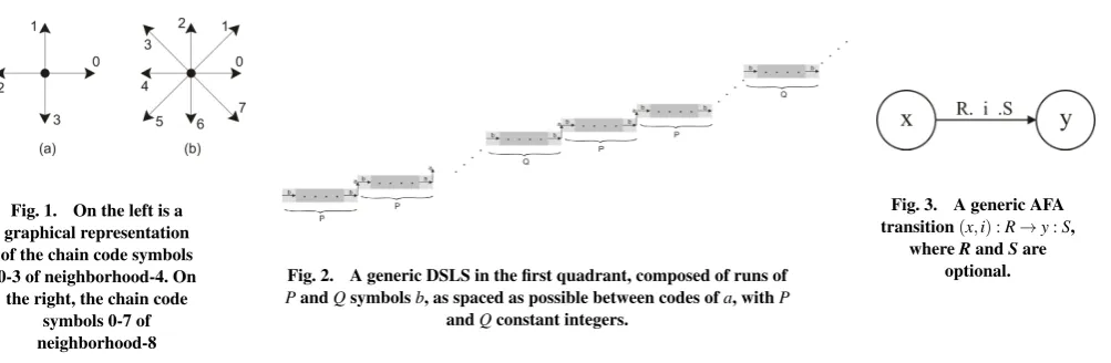
In search of a data structure that would reduce the number of primitives to be matched, [2] worked with an approach in image segmentation that produced a set of continuous digital lines rep-resented as chain codes which was the common data structure for representing complex segmentation results. Further work would concentrate on path planning to approximate the chains as se-quences of digitized straight line segments (DSLS1), with an algorithm in which the path is made up of straight line segments. Chain codewas introduced by Freeman in 1970 [9] as a one-pixel-thick boundary descriptor in a grid, and digital straightness was conjectured as well. In this model, given a pixel, the main and immediate neighborhoods of this pixel are shown by sym-bols, as in Fig. 1.
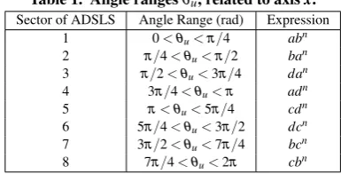
Fig. 2 shows an example of the string of DSLS in the first quad-rant, composed of symbolsaandb.
Fig. 1. On the left is a graphical representation of the chain code symbols 0-3 of neighborhood-4. On the right, the chain code
symbols 0-7 of neighborhood-8
Fig. 2. A generic DSLS in the first quadrant, composed of runs of
PandQsymbolsb, as spaced as possible between codes ofa, withP
[image:2.595.56.558.89.253.2]andQconstant integers.
Fig. 3. A generic AFA
transition(x,i):R→y:S,
whereRandSare
optional.
Understanding the problem from the syntactic point of view in-volves the concepts of language, grammar and types of gram-mars ([15]). According to Noam Chomsky, hierarchy dating back to 1956, languages are classified into four different classes: Re-cursive Languages (or type 0), Context Sensitive Languages (or Type 1), Context-Free Languages (or type 2) and Regular Lan-guages (or Type 3). There are degrees of complexity related to the classes mentioned since class 3 type is a subset of class Type 2, Type 2 class is a subset of a class type 1, class and type 1 is a subset of Class 0. Syntactic pattern recognition is one field that uses chain codes together with the rich theoretical background of languages, grammars and automata [30].
However, there are obstacles to employ the theory of languages, grammars and automata in robot navigation because DSLS are actually a very challenging subject incorporating all the dissim-ilarities and disparities between the discrete and the continuous representations [13].
For instance, DSLS of variable lengths require powerful recur-sive languages , making it impossible to apply simple formalism for syntactic analysis, such as FSA (finite state automaton) [6] -remarks that a regular language is specified by a regular gram-mar. The concepts of regular language and FSA are equivalent in the sense that for every regular language there is at least one FSA that recognizes it and vice versa [30].
Restricted to trajectories in only four directions (north, south, east or west), [26] investigated state machine applications in robotics introducing a syntactic method that used adaptability to dynamically increase the memory requirements. This work re-sulted in an architecture based on robot agents implemented by adaptive finite automata (AFA) as motion automata.
Overall, the scrutiny in studies and researches about robot nav-igation showed that the low representation fidelity using tradi-tional methods based on Cartesian environment maps results in little knowledge stored in the surroundings of the robot [18], commonly achieved by image processing sensors associated with detection of straight lines and arcs.
Yet, among the existing research approaches, syntactic meth-ods are usually considered unsuitable for tasks involving DSLS in robotic navigation. Since [8] and [7] presented capabilities of adaptive techniques related to the formalism of ADSLS in computational geometry, we advance further proposing this for-malism applied to robotic navigation utilizing the same AFA, a Turing-powerful device [19], such as motion automaton to direct robots.
This paper is organized as follows. In Section 2, the underlying principles necessary for understanding this study are presented, such as the state-of-the-art of DSLS and codification details. The method involved in this study is described in Sections 3 and 4, regarding automaton implementation and adaptive grids, respec-tively. Simulations are performed in Section 5 corresponding to proofs of concept aiming at the analysis of this proposal. In
Sec-tion 6, the posiSec-tion of this research within the state of the art is indicated. In Section 7, final considerations are drawn with in-tended future studies.
2. FUNDAMENTS
An adaptive device changes its behavior dynamically in response to input stimuli without interferences from other external agents, including users [19]. Normally, they are made of two layers com-prising a non-adaptive underlying mechanismND0, associated to an adaptive layerAM, using the same formalism of the first. This growth in complexity profits not only from the notable increment in expressive power of the combination, but also in versatility, as one can choose any consolidated mechanism as the non-adaptive device. An adaptive finite automaton(AFA) is represented by Expression 1 with FSA asND0.
AFA=(ND0,AM). (1)
The next topic presents a brief review of AFA.
2.1 Adaptive finite automaton (AFA)
From Equation 1, AFA is a rule-driven device described by a non-adaptive device, a FSA; associated to an adaptive layerAM comprisingadaptive actionsthat works on the original set of rules(ND0,AM).ND0characterizes AFA initial configuration. Adaptive actions are calls to parametric adaptive functions (ADF) responsible for self modification procedures. Depending on the stimulusifrom input string, linked to an operational step i, AFA configurationNDi−1is modified byadaptive actions, re-sulting that the FSANDi−1is changed to another FSANDi be-longing to the set{ND0,ND1,ND2,ND3...NDi....:i≥0}. Furthermore, the AFA formalism regards elementary adaptive actions to be applied to the transition set of the automaton, so that sets of elementary adaptive actions are abstracted in ADF which interconnects the adaptive layer toNDi, as presented in Fig. 3 through generic ADFRandS.
Fig. 3 shows the static graphic representation of a generic AFA transition wherexis the current state before the transition;yis the state after the transition;iis the input stimulus before the transition;Ris an ADF executedbeforeapplying the transition; and, finally,Sis an ADF executedafterapplying the transition. Graphically, any ADFRis portrayed byR•in case it is of the beforetype; likewise, any ADFSis anaftertype if it happens to be denoted by•S.
pattern from the current state set; and the insertion kind adds the pattern to the current set of transitions. A provision is made so that the inspection type is executed first, next the deletion, and finally the insertion kind; adding that null transitions have the lowest priority.
About ADF format, in the general case, it has a heading com-posed of parameters, generators and variables and a body con-stituted of elementary adaptive actions. All of them are optional; however, if parameters are specified, they have to be supplied to activate the corresponding ADF.
Variables are used in place of any of the components of the ele-mentary adaptive action, further assigned the actual correspond-ing values in the matchcorrespond-ing process with the pattern given. Then, after the matching process, variables may be undefined (in case no match is found) or defined (otherwise). Generators are used to assign names to newly created states. Roughly speaking, they are also like special variables, which are automatically assigned unique values as soon as an ADF is activated. In the activation of an ADF, the assignment of argument values to the parame-ters occurs, too. Neither generators nor parameparame-ters are allowed to change any longer, once assigned.
To differ from variables, generators receive the symbol∗as ex-ponent.
2.2 DSLS background
A digital arcSis understood as a set of interconnected pixels belonging to a digital image, positioned on a grid such that each point of the set has exactly two neighbors, except two of these points, known as extremes, which have only one neighbor inS [13].
Hence, in neighborhood-4 or neighborhood-8, the chain is a se-quence of elements in which each element is a symbol from Fig. 1 that represents the vector joining two neighboring pixels of a digital arch, aiming to represent the digital arch in question. In his model, Freeman stated that strings representing straight lines must obey three properties in neighborhood-8: (Prop1) At most two types of symbols, representing directions in the chain code, can be present, and these can differ by unity module eight. (Prop2) For one of these directions, the run length must be 1. One of the two symbols always occurs singly. (Prop3) Succes-sive occurrences of the single symbol are as uniformly spaced as possible among codes of the other value, which occurs in groups. The meaning ofProp1toProp3is to represent the straight line by a sequence of vectors with multiple slope of 450and the lengths of which are either 1 (when horizontal or vertical), or√2 (when diagonal).
As the third propertyProp3was considered somewhat unclear, researches proved that the straightness of a digital arc can be determined by the absence of unevenness in its chain code, nec-essary and sufficient for meeting the chord property2[12]. The chord property implied establishing a hierarchical structure composed of consecutive numbers corresponding to the runs and runs of runs of the symbols specified byProp1andProp2. This structure of consecutive numbers is expressed by an additional propertyProp4. [22] demonstrated that there can be only two possible lengths of these different runs, which are two consecu-tive integers (for example,PandP+1).
On the other hand, [13] showed examples of DSLS that violate the regularity implicit in the chord property, commenting that, in practice,Prop3andProp4are inviable in digital arcs. How-ever, it is more reasonable to expect a slight variation in the runs, within a tolerance level, but always keeping the overall slope, thus defining an approximate DSLS. Therefore, a criterion used
2A digital arcAis said to have the chord property if for every two digital pointscanddinA, and for each pointp= (x,y)oncd, there is a point e= (h,k)ofAsuch thatmax{|x−h|,|y−k|}<1 wherecdis the line segment betweencandd[22].
concentrated on strings that satisfied the first two properties of the conjecture, calledmonotonic codes, as they represent digital arcs that are either ascending or descending, with reference to coordinate axisxandy.
In order to keep the slope of a digital line, the smallest segment of a DSLS is called the Unit of the Straight Line Segment (USLS), resulting in mathematical models [16].
[7] and [6] stated an enhanced method taking into account that the adaptive representation can express changes in the scales of segments. Therefore, an irregular trajectory may be detected as DSLS after it is reviewed in a compatible scale, using metrics. In summary, adaptivity can be an alternative to incorporating the fundamentals of arithmetic discrete geometry to Freeman’s model in robot navigation.
2.3 Codification
If nothing else is specified, without loss of generality, in this pa-per neighborhood-4 (seeFig. 1) is the default, so that the symbols of propertyProp1must be consecutive, module four. More pre-cisely, the symbols that make up strings belong to∑={a,b,c,d}. To satisfyProp1, just consider module 4 along witha=1,b=0, c=3,d=2, for neighborhood-4 of Fig. 1 and Fig. 2.
Any stringS=s1....sn,si∈∑may be represented by its symbol, followed by the indication of itsi-th elementsigiving Expression 2:
S:si;i=1,2, ...,n. (2) In Expression 2,ndenotes the length of stringS, which means
|S|=n. Symbolssi∈∑may be called tokens, chain code ele-ments or stimuli, too. The null stringn=0 is represented byε. If all symbols ofSare identical,s=s1=s2=. . .=si=. . .=sn−1=sn, a compact representation isS=sn. Note that null transitions cause automaton non determinism, then symbols such as∆(∆∈/Σ) may be used in place ofε.
2.4 Adaptive DSLS (ADSLS)
AFA implements ADSLS related to digital paths of trajectories to represent the complexities of real world robot scenarios. ADSLS uses a modified chord property for models of higher orders (ordern) , thus incorporating tolerances in angle and in length of DSLS. The modified chord property changes neighbor-hood of chord property into a variable neighborneighbor-hood function such as max{|x−h|,|y−k|}<n, where nis the order of the model that depends on the momentary situation and the length of the segment, to sum up, of the stimuli. That is to say, the neigh-borhood function of DSLS must have a relatively large width , proportional to the measured length towards the overall linear structure [17].
Regarding techniques for error recovery in this study, it is of-ten convenient to represent the real numbers in a given circum-ference and not in a straight line, as usual. Especially, from the circumference of unit length, when defining an arbitrary origin point, we represent any pointT by its measured distance around the circle in a counterclockwise direction (this by definition). The division of the circle can be from the Farey series in the form ofspyrographsdescribed on page 326 of [13].
The techniques of error recovery of syntactic analysis of DSLS employ an approach similar to spyrographs in the form of adap-tiveloops, such that, by these loops, the circumference is built by states of the AFA, which moves cyclically and continuously through the closed loop. In effect, adaptive loops have their total number of states according to tolerance levels.
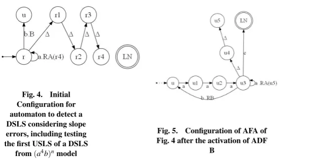
structural model. In the former case, the sequence should be ac-cepted; in the latter rejected. Fig. 4 exposes an AFA which tests the first USLS of a DSLS(a4b)n. Parameterr4is the last state of the HTST starting inr. From this arrangement, the AFA removes up to four∆transition by ADF RA. Elucidating, each time RA is activated by tokena, it removes from the automaton one of the ∆transitions that constitutes the HTST. Furthermore, any token breceived conducts the AFA to the final state; conditioned to if more than four tokensaare received, the sequence is rejected. The analysis of the other extreme is quite similar.
2.4.1 Slope errors and length similarity of DSLS. Recognition of DSLS subjected to slope errors is exemplified byU SLSi=
{anb: 3≤n≤5}.
Fig. 4 shows the initial configuration of the automaton prepared to accept truncatedU SLS1similar to the last item. With the first tokenbconsumed, ADF B is activated, which removes transi-tions of the initial configuration, changing the automaton topol-ogy to that of Fig. 5.
Afterwards, the AFA starts to consume the succeedingU SLSi: i>1 until the input stream is exhausted. A tokencis included just to signalize the end of the DSLS, when the automaton reaches the final state if the process is successful. On the other hand, if more than 5 tokensaare received,−[(xi,vr1):vr2−> vr3 :vr4]of RA removes transition ofcto the final state, reject-ing the sequence.
Strings of Fig. 6 show the performance of the AFA. These strings follow the modelU SLSi={anb: 3≤n≤5}, truncatingU SLS1 in some strings, too. Strings out of this model are rejected. Note that the AFA performance does not depend on the length of the input DSLS.
The method to represent and to apply tolerances is by a graph, or aloopsuch that the number of states of the loop (that is, its size) is changed adaptively in function, for example, of angleθS related to axisx; besides,θSgives the main direction of DSLSS, obtaining a syntactic measurement parameter(1−ψ)relative to S[6].
3. THE METHOD: APPLICATION TO THE
AUTOMATA
Software is modeled in this research as systems of state machines to cover the complete space environment of the robot, scheme adapted from [29]. The group of automata is necessary because there will be several alternative route options varying in angles. Independently of grid resolution changes the group of automata remains fixed either for routes in a relatively limited area or for routes over the complete area as well. Starting from an initial configuration, longer routes will dynamically increase the num-ber of automaton configurations, also increasing the numnum-ber of automaton states as shown in Fig. 6.
The validation of this study is made by simulations of robot movements associating robotic agents to motion automata, such as AFA, on account of a management system which supplies these agents with data. The technical details by which the man-agement system interconnects itself with AFA and the partition-ing criteria to implement AFA are described in the followpartition-ing items.
3.1 Architecture
In Expression 1, AFA is represented by two layers:
AFA=(ND0,AM), where AM is an adaptive layer; an adaptive structure was implemented to simulate navigation scenarios composed of the following layers:
—The System Manager is a hierarchically superior adaptive layer to monitor and to coordinate ADSLS, such as the amount of ADSLS changes according to the stimuli under manage-ment of this layer. The System Manager searches information
from ADSLS in their respective final states, which indicate if the input string was accepted or rejected;
—The Slave Layer comprises one or more ADSLS and it is com-manded by the System Manager or adaptive upper layer.
In the more general case, the upper layer controls the ADSLS of the slave layer by strings of typeW=ΨC.
Ψis a chain code received by the AFA in order that this one adjusts a tolerance band related to the chainC.Ψcorresponds to a factor to compensate for inaccuracies in the digitalization process. The subject of inaccuracies and errors in digitalization is detailed in [8], which lists several papers on this issue.
3.2 Design patterns
[image:4.595.331.524.349.447.2]Topic2.4.1 illustrated the recognition of DSLS subjected to slope errors, exemplifying by ADSLS of U SLSi={anb: 3≤n≤5} with 3 a transitions and(5−3)∆transitions. That adaptive structure (automaton of Fig. 5) is one of the design patterns of this method because to implement other structures from other quadrants, it is just necessary to change the symbols of the pattern conveniently, obtaining an ADSLS with the same topology. Table 1 shows angle ranges of ADSLS and respective expressions of USLS that helps in this procedure.
Table 1. Angle rangesθu, related to axisx. Sector of ADSLS Angle Range (rad) Expression
1 0<θu<π/4 abn 2 π/4<θu<π/2 ban 3 π/2<θu<3π/4 dan 4 3π/4<θu<π adn 5 π<θu<5π/4 cdn 6 5π/4<θu<3π/2 dcn 7 3π/2<θu<7π/4 bcn 8 7π/4<θu<2π cbn
Simply, for example, to implement an ADSLS for angle range between5π/4and3π/2radians, just change the symbols of the pattern of Fig. 5 in the following way:atocandbtodgetting the ADSLS with the same topology (belonging to the third quadrant). In a quadrant, for instance for angles between0andπ/2 radi-ans, grant the validity of propertiesProp1andProp2, conceiving that symbols change atπ/4radians by inspection in Table 1. 3.3 Partitioning criteria to implement ADSLS
The partitioning criteria to implement AFA is in compliance with the angle ranges of each ADSLS to cover2π radians, ponder-ing about angle errors of DSLS and requirponder-ing precision, as well. Topic 2.4.1 exemplified the ADSLS with U SLSi={anb: 3≤n≤ 5}.
If angles of DSLS are between0andπ/2radians in this topic, inasmuch as a similar behavior occurs in other quadrants:i) For 0<θu<π/4, U SLSi=abn, implyingθu=arctan(1/n);ii) For π/4<θu<π/2, U SLSi=ban, implyingθu=arctan(n). Then approximations are by virtue of non-linearity and discontinuity of the function arctangent.
Accordingly, with nmin≤n≤nmax for sectors S1, S4, S5, S8, Expression of angle rangeθuof USLS is:arctan(1/nmax)≤θu≤ arctan(1/nmin). With nmin≤n≤nmaxfor sectors S2, S3, S6, S7, Expression of angle rangeθu of USLS is:arctan(nmin)≤θu≤ arctan(nmax).
3.4 Implementation of Automata
Fig. 4. Initial Configuration for automaton to detect a DSLS considering slope errors, including testing the first USLS of a DSLS
from(a4b)nmodel
Fig. 5. Configuration of AFA of
Fig. 4 after the activation of ADF B
Fig. 6. Examples of DSLS
produced by U SLS={anb: 3≤n≤5}, accepted by AFA of Fig. 5
±π/2radians, anglesθuof DSLS greater thanθ1e =arctan(20) are approximated to+π/2or−π/2radians, each one to be an-alyzed depending on the sector. For angles of sector 1, 4, 5 and 8, anglesθuof DSLS smaller thanθ2e =arctan(1/20)are approxi-mated to0orπradians, to be analyzed depending on the sector. Implemented automata are described below.
3.4.1 ADSLS. For the first quadrant, refering to Table 1, the following ADSLS were selected.
Sector 1 (abn):2≤n≤4(Automaton A);5≤n≤7(Automaton B);8≤n≤12(Automaton C);13≤n≤20(Automaton D). Sector 2 (ban):2≤n≤4(Automaton A);5≤n≤7(Automaton B);8≤n≤12(Automaton C);13≤n≤20(Automaton D). For the other quadrants, the same topology as that of the ADSLS of the first quadrant was chosen implying each sector has 4 au-tomata: Automaton A, Automaton B, Automaton C, Automaton D.
[image:5.595.98.240.542.587.2]3.4.2 For angles(0+kπ/2) radians , with k=0,1,2,3, .... For 0 radians, straight line is of the kind: aaaaaaa....; forπ/2: bbbbbbb...; forπ: ddddddd...; for3π/2: ccccccccc..., requir-ing 4 automata for the syntactic analysis of these languages. For 0 radians, language of straight line strings is L={an:n>0}. Fig. 7 shows an automaton which accepts L:
Fig. 7. Finite accepter that recognizes the set of strings belonging
toL={an:n>0}, for0radians.
In Fig. 7, with the first symbol a, the automaton goes into state 2, staying in this state for symbols a, accepting the input string. Any symbol b,c,d which received the automaton enters state 3, a non-final trap state, signifying the input string is rejected. The other automata have the same topology, changing the sym-bols conveniently.
3.4.3 For angles(π/4+kπ/2)radians , with k=0,1,2,3, .... Forπ/4radians, straight line is of the kind: abababababab....; for3π/4: bcbcbcbcbcbcb...; for5π/4: dcdcdcdcdcdcd...; for 7π/4: cbcbcbcbcbcbcbcbc.... Fig. 8 is an automaton that accepts strings forπ/4radians:
In Fig. 8, with symbols ab or ba, the automaton enters final state 4 or 5, respectively. In state 4, the input string is accepted as long as symbols ab are received in sequence. Final state 6 allows the automaton to accept an a symbol ending the input string. In state
5, the input string is accepted as long as symbols ba are received in sequence. Final state 7 allows the automaton to accept a b symbol, the last one of the input string. Non-final trap states are not included.
The other automata have the same topology, changing the sym-bols conveniently.
4. THE METHOD: APPLICATION TO THE GRID
MAP
Observing that the chain code symbols 0-3 of neighborhood-4 or chain code symbols 0-7 of neighborhood-8 of Fig. 1 are the primitives that define the grid resolution, [18] points out of those grids are considered relatively simple data structures that pro-vide a comprehensive picture of the surfaces in the continuous terrain for robot navigation in a dynamic environment. How-ever, paths formed by grid edges can be longer than true short-est paths in the terrain since their headings are artificially con-strained, restricted to multiples of 45 degrees [18].
The improvement in robot navigation is proposed here by the following: i) Bringing ADSLS into play . ii) Concurrently, us-ing adaptive grid resolution. iii) Linked together, applyus-ing adap-tive changes of orientation angles related to the environment of graphical representation of the chain code symbols 0-3 of neighborhood-4 or chain code symbols 0-7 of neighborhood-8, of Fig. 1.
Item i) above avoids the movement in constrained angles (4: angles multiples of 90 degrees, neighborhood-8: angles multiples of 45 degrees). Item ii) varies grid resolution depending on the trajectory, adaptively changing the length of the chain code symbols of Fig. 1. Item iii) is to escape the lim-itation caused by the discontinuity of the arctangent function, adaptively changing the angle of the chain code symbols of Fig. 1.
Strings resulting from the adaptive scale factor changing the length of primitives are recognized by the same set of automata: spatial variability of grid by adaptivity does not require chang-ing the automata.
By being limited to regular languages, [30] had to introduce a scale normalization factor, which could be the total length of a trajectory pattern. A scale transformation in the work by [30] aims to identify the similarity between contours (trajectories) by their corresponding pattern attributes (descriptors) after under-going the transformation.
con-text, a technique of [30] known since the 1970s granted by im-provements in computational power obtained by adaptivity.
5. EXPERIMENTS
The minimum grid resolution planned for this work is of the robot dimension order, which involves a question of compatible scale between each step of the robot motion and their respective di-mensions.
5.1 Method proposed by this research
In the classical method, for moving from a starting point to a des-tination point, the robot has to find a path for which the computa-tional cost is minimum because this is the path with the shortest distance, too. To compute a minimum cost path, it is necessary to compute robot moves from each cell grid to one of its neighbor cells by changing directions, or transitions, from cell to cell. Af-terwards, the algorithm computes the total cost in reaching the destination in one of the shortest paths.
A didactic way to describe the method proposed in this pa-per is to consider that the robot moves every USLS of the trajectory chain input (segmented in DSLS), instead of mov-ing by each symbol as in the classical method. It implies that the robot travels a path consisting of points corresponding to each USLS. It follows that, given an input with nUSLS:
{U SLS1,U SLS2,U SLS3,U SLS4,U SLS5, ...,U SLSn}, the robot will have n short moves to reach the end point, which means computational cost gains regarding traditional methods. A better solution, computationally more effective than the earlier one, is driving the robot directly to the final point; therefore, this case involves exchanging information with the robot only about coordinates indicative of the map location only of the end point. In short, the method proposed here uses the ADSLS model since, for moving from a starting point to a destination point, the path is segmented in straight line segments, considerably reducing com-putational costs. This can be seen in Fig. 9, which shows the same robot in two different positions of the same trajectory, with classical method moves indicated by dashed lines and, in red, the single move by the method proposed by this study.
In all robot figures, the classic method trajectory is indicated in dashed lines and in red is the resulting trajectory proposed by this paper.
5.2 Adaptive grids
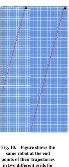
The effect of adaptive grids may be seen in Fig. 10 that shows the same robot at the end points of their trajectories in two different grids.
Fig. 13 shows a robot in a trajectory segmented into three DSLS (chain 1, 2, 3) in the same scale. Chain 1 is DSLS1=a2ba4ba3ba4ba3ba3ba4ba3ba4ba4b recognized by Au-tomaton B- sector2. Chain 2 is DSLS2= (cb5)(cb6)(cb6)(cb7) recognized by Automaton B-sector8. Chain 3 is DSLS3 = (c8b)(c9b)(c12b)4 recognized by Automaton C-sector7, de-scribed in topic 3.4.1 and Table 1
Figure 11 and Fig. 12 is the same robot of Fig. 13, although chain 3 is in scale 0.5 and 1.5, respectively.
6. COMPARISON WITH EXISTING
TECHNIQUES
This topic indicates the position of this research within the state of the art, inferred by comparison with selected works as the ones mentioned in item 1 taking in consideration that studies in robot navigation generated two major paradigms for mapping indoor environments: grid-based and topological. An overview of the state of the art is provided by [1].
In the occupancy grid method, space may be referred to the vicin-ity of the robot described by local parameters, or to the entire
space by global parameters normally by exploring the environ-ment [24].
Based on the fact that occupancy grids tends to be both unreli-able and computationally expensive, [24] reports experiments with four techniques for position estimation using occupancy grids. [18] highlighted that the trajectories of robots require varying angles of trajectories (labeled as navigation at "any-angle"). Thus, [18] states that the trajectories on the Cartesian grid tend to be not the shortest path (ie, the shortest paths on the terrain) because trajectories are restricted artificially to multi-ple angles of 45 degrees (8-neighborhood) or multimulti-ples of 90 de-grees (4-neighborhood). In another study with the same purpose of angles in variable trajectories, [28] formalizes a search space of alternative routes through a search algorithm on graphs. Problems in world modeling techniques based in grid methods resulted in combining global and local occupancy grids [24] and in topological maps. [27] says that topological maps can be used much more efficiently than grid methods. However, techniques based on topological maps provide a limited accuracy because of the low granularity of the discretization [4]. Since topologi-cal maps are considerably difficult to learn in large-stopologi-cale envi-ronments, [27] describes an approach that integrates grid-based and topological approaches.
Hence, an existing tendency is to join local metric maps, espe-cially grid-based, through a global topological map. This ten-dency is not new, as [14] describes an approach by which metri-cal information is then incrementally assimilated into lometri-cal ge-ometric descriptions of places and edges, and finally merged into a global geometric map. With this representation, [14] in-forms that successful navigation does not depend critically on the choice of sensors and movement actuators, their accuracy, or even on the existence of the geometrical descriptions. Regarding adaptive techniques using AFA in mapping trajecto-ries, certainly the state of the art is represented by [26] which is restricted to trajectories in only four directions (north, south, east and west), sufficient for its purpose. The motivation of [26] in using adaptivity was due to the high amount of memory for recording information for mapping environments required by path planning systems on grids.
The scheme proposed here also involves the formalization of a search space of routes with certain analogy with [28], but this space is represented in this study by an adaptive neighborhood expressed by AFA states. This study proposes to apply the formal-ism of ADSLS to enable navigation at any angle as in [18] and [28] , however integrating in the framework the positive points obtained by [26] in enabling the use of adaptivity to progres-sively use system memory, consumed according to the area al-ready mapped.
In addition, the formalism of ADSLS presents other advantages in memory usage, considering that just registering coordinates of only two points, the endpoints of the segments representing digitized trajectories, is enough, and not the record of all the points of the trajectories to map building. These advantages in memory usage can contribute to solving the greatest drawback of grid-based approaches, with their enormous space and time complexity, mentioned by [27].
When it comes to syntactic devices, trajectories varying in angle with relatively any length prevent the use of finite automaton for the purpose of this study and inhibits automaton solutions in data structures for robot navigation. In the opinion of [11], the capa-bility of a more powerful class of formalisms should rejuvenate syntactic research originally pursued in the 70s-80s.
Fig. 8. Finite accepter that
recognizes strings forπ/4
radians.
Fig. 9. The figure shows
one robot in two different positions of the same trajectory: the classical
method trajectory is indicated in dashed lines and in red is the resulting
trajectory proposed herein. On the left is an intermediary position, and
on the right the end position for the input
stringDSLS=
a3ba5ba3ba4ba3ba3ba4ba3ba5ba4b recognized by the
[image:7.595.389.504.118.396.2]automaton of Fig.5
Fig. 10. Figure shows the
same robot at the end points of their trajectories
in two different grids for
input stringDSLS=
a3ba5ba3ba4ba3ba3ba4ba3ba5ba4b recognized by the
automaton of Fig.5
by rules (with multi-level hierarchical adaptivity) whose set of rules is modifiable presenting variable adaptive functions. Concluding, comparing with the traditional models, without adaptivity, this work has the following objectives: i) Flexibility: In general, traditional methods tend to be computationally com-plex and too susceptible to errors, spurious interferences, ac-curacy of sensors and models. Dynamic changes in the vicinity of theoretical models, which alter the functionality of the algo-rithms depending on the stimuli, allow better characterization of global attributes; ii) Computational Complexity: The introduc-tion of adaptive tolerances simplifies the algorithms compared to methods with invariable behavior, reducing complexity of tive algorithms; iii) The advantage of adaptive scale: The adap-tive scale allows access to local and global information. Therefore, this comparison with selected or classical works, rep-resententing tendencies of the state of the art, shows a whole evo-lutionary potential of this proposal, just by integrating the for-malism of adaptive straightness to the traditional models without adaptivity.
7. FINAL CONSIDERATIONS
Despite the significance of computational representation, the DSLS being an active area of research for almost half a cen-tury as the surveys [13] and [3], this issue has not been ex-plored in robotic navigation for scenarios subjected to spurious influences, with adaptive resources listed in [19]. This research fulfills this gap by incorporating the fundamentals of arithmetic discrete geometry [21] in the syntactic method for robotic navi-gation, through adaptive techniques.
Indeed, considering variable angles and minute errors of DSLS, to our knowledge, this is the first attempt to introduce AFA in robot navigation. By traditional techniques, automata would have to be implementeda-priori, with high level of complexity to treat errors that cause imprecise models or imprecise scale of DSLS in different angles.
Compared with other methods of digital line representation in navigation, this work showed that the formalism presented in [8] opens new possibilities for robotics navigation, incorporating the main advantages of the ADSLS formalism: i) Simplicity and relative ease of modeling and implementation, associated with high computational power; ii) Models are easy to understand, relatively simple to program and flexible to accept changes in their behavior; iii) Longer trajectories will dynamically increase the storage mapping memory used; iv) Storage memory required to map unknown environments may be reduced drastically by adaptive straight line segmentation of trajectories because just two grid coordinates are necessary to describe a specific digi-tized straight line path.
Fig. 11. Figure shows the same robot as in Fig. 13 in a trajectory segmented in three DSLS (chain 1, 2, 3) with chain 3 in scale 0.5. In
all robot figures, classic method trajectory is indicated in dashed lines and in red is the resulting
trajectory proposed herein.
Fig. 12. Figure shows the
same robot as in Fig. 13 and Fig. 11 in a trajectory segmented in three DSLS (chain 1, 2, 3) with chain 3 in
scale 1.5.
Fig. 13. Figure shows a
robot in a trajectory segmented into three DSLS (chain 1, 2, 3) in the
same scale, recognized by three automata.
obstacles in trajectories, and experimentation of simulated algo-rithms in real robots.
8. REFERENCES
[1] Alejandra Barrera.Advances in Robot Navigation. InTech, 2011.
[2] Rudiger Befit, Dietrich Paulus, and Michael Harbeck. Seg-mentation of lines and arcs and its application for depth recovery. InAnais..., volume 4, pages 3165 –3168 vol.4. IEEE International Conference on Acoustics, Speech, and Signal Processing, ICASSP-97, april 1997.
[3] Partha Bhowmick and Bhargab B. Bhattacharya. Fast polygonal approximation of digital curves using re-laxed straightness properties.IEEE Transactions on Pat-tern Analysis and Machine Intelligence, 29:1590–1602, September 2007.
[4] Wolfram Burgard, Dieter Fox, Daniel Hennig, and Timo Schmidt. Estimating the absolute position of a mobile robot using position probability grids. InIn Proceedings of the Thirteenth National Conference on Artificial Intelligence, Menlo Park, pages 896–901. AAAI Press/MIT Press, 1996. [5] Yeong-Hwa Chang, Tsu-Tian Lee, and Chang-Huan Liu. On-line approximate cartesian path trajectory planning for robotic manipulators.IEEE Transactions on Systems, Man, and Cybernetics, 22(3), may 1992.
[6] Leoncio C. de Barros Neto, André R. Hirakawa, and Anto-nio M. A. Massola. Adaptive modeling of digital straight-ness applied to geometric representation enhancement. In-ternational Journal of Computer Applications, 10(2):31– 39, November 2010. Published by Foundation of Computer Science.
[7] Leoncio C. de Barros Neto, André R. Hirakawa, and An-tonio M. A. Massola. An adaptive model applied to digi-tal geometry to enhance segment straightness.IEEE Latin America Transactions, 9:956 – 962, Oct. 2011.
[8] Leoncio Claro de Barros Neto.Modelagem em geometria digital aprimorada por técnicas adaptativas de segmentos de retas. PhD thesis, Escola Politécnica da Universidade de São Paulo (USP), Junho 2011.
[9] H. Freeman. Boundary encoding and processing.Picture Processing and Psychopictorics, pages 241–266, 1970. B.S. Lipkin and A. Rosenfeld, editors, New York, Academic Press, 1970.
[10] Bartolomé Garau, Alberto Alvarez, and Gabriel Oliver. Path planning of autonomous underwater vehicles in cur-rent fields with complex spatial variability: an A* ap-proach. InICRA, pages 194–198. IEEE, 2005.
[11] Feng Han and Song Chun Zhu. Bottom-up/top-down im-age parsing with attribute grammar.IEEE Transactions on Pattern Analysis and Machine Intelligence, 31(1):59–73, January 2009.
[12] S.H.Y. Hung. On the straightness of digital arcs. IEEE Transactions on Pattern Analysis and Machine Intelli-gence, PAMI-7(2):203–215, March 1985.
[13] Reinhard Klette and Azriel Rosenfeld.Digital geometry: geometric methods for digital picture analysis. Morgan Kaufmann, 2004.
[14] Benjamin Kuipers and Yung-Tai Byun. A robot explo-ration and mapping strategy based on a semantic hierar-chy of spatial representations.Journal of Robotics and Au-tonomous Systems, 8:47–63, 1991.
[16] Shu Xiang Li and Murray H. Loew. Analysis and model-ing of digitized straight-line segments. In Anais..., pages 294–296, Rome, Italy, 1988. Proceedings of International Conference on Pattern Recognition, Publ by IEEE, Piscat-away, NJ.
[17] Peter F.M. Nacken. Metric for line segments.IEEE Trans-actions on Pattern Analysis and Machine Intelligence, 15(12):1312–1318, December 1993.
[18] Alex Nash, Kenny Daniel, Sven Koenig, and Ariel Felner. Theta*: Any-angle path planning on grids. In National Conference on Artificial Intelligence, pages 1177–1183, 2007.
[19] J. J. Neto. Um levantamento da evolução da adaptativi-dade e da tecnologia adaptativa.Revista IEEE América Latina, 5(7):496–505, Novembro. 2007.
[20] J. J. Neto. Adaptatividade: generalização conceitual. In Anais..., Escola Politécnica da Universidade de São Paulo, 2009. 3oWorkshop de Tecnologia Adaptativa (WTA). [21] J. P. Reveillès.Géométrie discrète, calcul en nombres
en-tiers et algorithmique. PhD thesis, Université Louis Pas-teur, Strasbourg, 1991.
[22] Azriel Rosenfeld. Digital straight line segments. IEEE Transactions on Computers, C-23(12):1264–1269, Decem-ber 1974.
[23] N. Sariff and N. Buniyamin. An overview of autonomous mobile robot path planning algorithms. In Anais... 4th Student Conference on Research and Development, June 2006.
[24] Bernt Schiele and James L. Crowley. Comparison of po-sition estimation techniques using occupancy grids. InIn Proceedings of the 1994 IEEE International Conference on Robotics and Automation, pages 1628–1634, 1994. [25] J. Sellen. Direction weighted shortest path planning. In
Anais..., volume 2, pages 1970 –1975 vol.2. IEEE Interna-tional Conference on Robotics and Automation, may 1995. [26] M. A. A Sousa, A. R. Hirakawa, and J. J. Neto. Adaptive automata for mapping unknown environments by mobile robots. InAnais... Ibero-American Conference on Artifi-cial Intelligence, Lecture Notes in ArtifiArtifi-cial Intelligence: Advances in Artificial Intelligence, p.562-571, 2004. [27] Sebastian Thrun and Arno Bü. Integrating grid-based and
topological maps for mobile robot navigation. In Proceed-ings of the Thirteenth National Conference on Aartificial Intelligence - Volume 2, AAAI’96, pages 944–950. AAAI Press, 1996.
[28] Kamil Tulum, Umut Durak, and Kemal Ider. Situation aware uav mission route planning. In IEEE Aerospace con-ference, editor,IEEE Aerospace Conference, March 2009. [29] Ferdinand Wagner, Ruedi Schmuki, Thomas Wagner, and Peter Wolstenhoime.Modeling Software with Finite State Machines: a Practical Approach. Auerbach Publications, 2006.