A dynamic general equilibrium model for tax policy analysis in Colombia

Munich Personal RePEc Archive

A dynamic general equilibrium model for

tax policy analysis in Colombia

Hernandez, Gustavo Adolfo and Light, Miles and Rutherford,

Thomas

Departamento Nacional de Planeacion, Ministerio de Hacienda

Republica de Colombia

May 2002

República de Colombia

Departamento Nacional de Planeación

Dirección de Estudios Económicos

ARCHIVOS DE ECONOMÍA

A dy namic general equilibrium model for tax policy

analy sis in Colombia

Miles K. LIGHT

Gustavo Adolfo HERNANDEZ

Documento 189 15 de Mayo de 2002

La serie ARCHIVOS DE ECONOMIA es un medio de la Dirección de Estudios Económicos, no es un órgano oficial del Departamento Nacional de Planeación. Sus documentos son de carácter provisional, de

A Dynamic General Equilibrium Model for

Tax Policy Analysis in Colombia

Thomas F. Rutherford and Miles K. Light

University of Colorado

Gustavo Hern´andez

May 10, 2002

Abstract

The paper documents a dynamic general equilibrium model for Colombia based on national accounts from 1999. The paper is part of a project in-tended to develop a capacity for the the design, specification, and application of computable models within the Colombian Ministry of Finance and Depart-ment of National Planning. Our analytical framework includes both forward-looking expectations and Harris-Todaro labor markets. In the present paper we compare numerical results from the dynamic model with simpler static and steady-state formulations to highlight the importance of transitional effects in evaluating tax policy reform. Our applications include measurement of the marginal cost of funds from different tax bases and the evaluation of discrete changes in tariff structure. The structure of the labor and intermediate credit markets have important implications for the ranking alternative tax reform proposals.

∗_{The authors would like to thank Sergio Prada and Juan Mauricio Ram´ırez from Ministry of}

1

Introduction

This paper introduces a multi-sectoral, dynamic general equilibrium model for tax policy analysis in Colombia. The model incorporates Harris-Todaro migration and unemployment and two alternative representations of international capital flows, issues which are important considerations for tax reform in developing countries such as Colombia. While the analysis presented in the paper provides policy-relevant insights, the primary objective of the paper is pedagogic. We have developed a template model which can provide a starting point for a variety of future studies of the Colombian tax system.

There are two illustrative calculations reported in this paper. The first compares the marginal cost of funds (MCF) from Colombia’s major tax streams. Here we find that one peso of public funds costs 1.2 to 5 or more pesos of foregone current and future consumption, depending on the tax instrument used to raise the revenue, the time horizon of the model, and the labor market formulation. In a second set of illustrative calculations we evaluate two alternative tariff-reform policies. The first policy provides tariff exemptions for capital- and high-tech imports which is intended to foster capital accumulation while the second moves toward a more uni-form tariff structure, lowering tariff rates on some goods and raising rates on others. In a second best context, economic theory does not indicate which of these policies would be preferred, but our computable framework indicates that a movement to-ward uniformity presents substantial efficiency gains while the movement away from uniformity results in a loss of efficiency and fails to promote growth.

We do not put forward these policies as a particular tax reform agenda. Our intent is only to illustrate how the model might be applied to evaluate specific tax reforms. We leave future applications of the modeling framework to specific tax proposals to our colleagues in the Ministry of Finance and the Department of National Planning.

In order to highlight the role of the intertemporal margin on capital taxes, we compare the results from the forward-looking dynamic model with the same policy experiment analyzed in the context of the static and steady-state models.1

The

1_{See Rutherford and Tarr [2001] for a similar analysis for Chile of the differences between policy}

dynamic model tracks a transition between the short and long-run equilibria. For many experiments, the cost of a distortionary tax policy is larger in a dynamic model than a static model because capital accumulation increases the distortionary effect. Conversely, the transitional impacts are typically smaller than in a steady-state model because the framework accounts for the cost of capital accumulation, while this is only partially accounted for in the steady-state model.

We work in the framework of a classical Ramsey analysis of optimal economic growth with perfect foresight. This is a natural starting point because of the generic representation of financial markets. The model represents an open economy with perfect competition in all markets, a representative consumer, and a constant rate of technological progress. The underlying theoretical model is well studied in the economics literature.2 _{This model is intended to provide a starting point for future}

quantitative policy analysis, and we therefore have made a number of simplifying assumptions to maintain transparency.

This paper compares results from a collection of related yet distinct models, it is helpful to lay out the logical framework in some detail so that the similarities and differences in model structure are readily apparent. We therefore begin with a schematic overview of the equilibrium structure and benchmark data for the static model.3

Thereafter we lay out the equations which characterize the steady-state and dynamic extensions of the static model. After going through the model formulations, we consider two illustrative applications of the model for policy analysis. Appendices are provided which cover programming details related to the implementation of dynamic models in GAMS/MPSGE and instructions for running the model.

2_{See, for example, Blanchard and Fischer [1989], and Barro and Sala-i Martin [1995]. The}

numerical representation of this model is less common in textbooks. See Lau et al. [2002] for an introduction to dynamic equilibrium modeling in a complementarity format. Harrison et al., eds [2000] contains a collection of papers based on policy-oriented dynamic general equilibrium model-ing. The present analysis does not address the connection between tariff reform and productivity growth as in Rutherford and Tarr [2002], but such an extension of the present model could be quite useful.

2

The Static and Steady-State Models

The static model for Colombia represents an Arrow-Debreu economy with constant returns-to-scale and perfect competition. The model is based on 1999 Colombian national accounts which distinguish 16 industries, government, and a single repre-sentative household. Equilibrium in this model is characterized by a set of prices and levels of production in each industry such that the market demand equals sup-ply for all commodities. Producers are assumed to maximize profits, there is free entry, and production exhibits constant returns to scale, hence no activity earns a positive economic profit at equilibrium prices. Following Mathiesen (1985) we for-mulate and solve as a complementarity problem in which three types of equations define an equilibrium: market clearance, zero profit, and income balance.

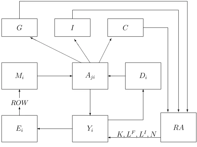
The relationship between different blocks of a typical model is shown in Figure 1. Taxes are discussed in the next section and therefore, for simplicity, do not appear in this figure.

Ei ✻ ROW ✻ Mi Yi Di Aji RA

G I C

✛ ✲ ❄ ✛ ✻ ✛ ❍ ❍ ❍ ❍ ❍ ❍ ❍ ❍ ❍ ❨ ❏ ❏ ❏ ❏ ❪ ✁✁ ✁✁✕ ❄ ❄ ❄

K, LF_{, L}I_{, N}

Fig. 1. Flows in a static model

Sector’s i output (denoted Yi) is produced using capital Ki, formal labor LF i , informal labor LI

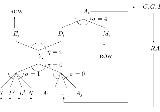
of domestic goods Dj and imports Mj. This same composite good enters private consumption C, government consumption G, and investment I. Output from Yi includes Di and Ei. A representative agent RA represents a collective decision process for allocating income to households and to a government. The representative agent has an endowment of capital K, two types of labor (LF _{and L}I_{) and tax} revenue (not shown). The same consumer demands C, I and G.

Production sector Yi produces two types of commodities: domestic goods Di and goods for export Ei. These goods are assumed to be imperfect substitutes, produced with a constant elasticity of transformation. For production, each sector uses capital, labor, land and intermediate goods. As such, the sector’s iproduction function is

Yi =g(Di, Ei) =f(Ki, LIi, LFi , Ni, Aji) (1) where g is a constant-elasticity-of-transformation function for outputs, and f is a nested Leontief - Cobb-Douglas production function for inputs. Capital, labor and land enter as a Cobb-Douglas value-added aggregate. Intermediate inputs and the value-added composite enter as a Leontief aggregate at the top level.

The representative consumer demands investment, private and government goods, and receives transfers from the government. In the static model investment is ex-ogenous, while private demand is determined by utility-maximizing behavior. (Con-sumer utility consists of a Cobb-Douglas utility index defined over Armington ag-gregations of domestic and imported commodities.) In the static model investment is exogenously fixed. In all the models, the level of public provision is held constant, and all tax policy analysis is undertaken subject to an equal yield constraint. When one tax rate is reduced, another tax flow is increased to compensate for the lost revenue.

K LF _LI _N ¡¡ ¡ ☞☞ ☞ ▲ ▲ ▲ ❅ ❅ ❅

A1 ... Aj

¡¡ ¡ ☞☞ ☞ ▲ ▲ ▲ ❅ ❅ ❅ ✦✦✦✦ ✦ ❛ ❛ ❛ ❛ ❛ Yi ✦✦✦✦ ✦ ❛ ❛ ❛ ❛ ❛

Ei Di Mi

✻ row Ai ✻ row ✦✦✦✦ ✦ ❛ ❛ ❛ ❛ ❛ ✲ ✻

C, G, I

✚✙

✒ ✑ ✒ ✑

✚✙

✛✘

σ= 1 σ = 0

σ = 0

η = 4

σ = 4

❄

RA

✻ ✻ ✻ ✻

Fig. 2. Structure of the static model

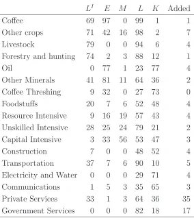
Table 1 presents a perspective on the sectoral shares of economic activity in 1999. Here we see that as in many developing countries, GDP is generated primarily in agriculture, resource-intensive and and service sectors. High tech / capital intensive manufacturing accounts for only 3% of value-added but 57% of imports. The key exports in 1999 were agricultural goods plus coffee (25% of export earnings) and oil (22%). Over half of formal labor is employed in service sectors, a third of which is in the public sector. Informal labor is largely employed in agricultural sectors (40%) and private service sector (45%).

The input-output data indicate that capital formation is based on inputs of con-struction services and high technology/capital-intensive manufactured goods. Final demand is composed of services (33%), foodstuffs (19%) and various manufactured goods (27%).

Table 2 describes the primary factor and trade content of various sectors in the economy. Informal labor earns a relatively large share of aggregate wage payments in agricultural sectors which are highly export-oriented. For example, 69% of wage payments in the coffee sector are to informal workers, and 97% of coffee output is exported.

untraded.

The capital value share column indicates the relative importance of capital in the oil sector (77%) and for selected services (electricity is 71%, communications 65%). The manufactured goods have capital value shares ranging from 20 to 50%.

In the model implementation we include the option to distinguish base year capital earnings between returns to physical capital and returns to sector-specific resources. For example, it would not be appropriate to assume that all capital earnings in the oil sector necessarily accrue to physical capital, otherwise we would be assuming that an expansion of the sector only would require additional oil wells and not new oil fields on which to place the wells. The scenarios described here do not utilize this feature.

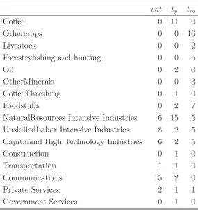
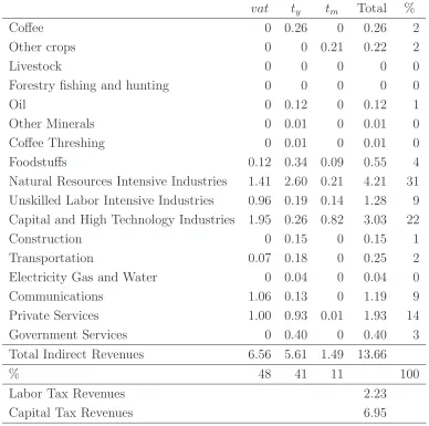
Tables 3 and 4 describe the structure of direct and indirect taxes. Table 3 fo-cuses on sectoral tax rates as they apply to value-added, output and inputs. The term “VAT” is used somewhat loosely, as the model and actual application of this tax is on agggregate demand rather than on sectoral value-added. While the posted value-added tax rate is 16%, the base year data suggest that the VAT tax is applied primarily on manufactured goods and communication services. Agricultural prod-ucts, oil and most services are exempt, yet (as indicated in Table 4), this tax base contributed nearly half of all indirect tax revenues in 1999.

Excise taxes apply on the value of production, both on sales in the domestic economy and on exports. Excise taxes apply at the highest rate on natural resource-intensive manufactures (15%) and coffee (11%). Looking at tax revenue (Table 4), we find that given the relative size of sectors, the single most important indirect tax in the economy is the excise tax on natural resource intensive production, a tax which generated 2.6 billion pesos in 1999.

In 1999 tariffs were applied at a 5% rate on manufactured goods imports and 16% on agricultural goods. In terms of collected revenue, the tariff instrument contributes a relatively small amount, only 11% of all indirect tax revenue.

Table 1: Shares of Economy-Wide Totals (%)

Value

Added LF LI K E M G I C

Coffee 1 1 4 0 8 0 0 -2 0 Othercrops 7 4 18 0 17 5 0 5 4 Livestock 4 1 13 1 0 0 0 4 1 Forestry and fishing 1 0 2 0 0 0 0 3 0

Oil 4 2 0 5 22 0 0 0 0

OtherMinerals 2 1 3 1 9 0 0 0 0 CoffeeThreshing 0 0 0 0 1 0 0 2 0 Foodstuffs 4 3 3 6 5 4 0 4 19 Natural Resources 4 5 1 3 10 14 0 3 10 Unskilled Intensive 2 3 2 2 7 9 0 4 9 Capital and High Tech 3 3 0 4 14 57 0 29 8 Construction 4 4 1 8 0 0 0 43 0 Transportation 5 7 8 2 3 3 0 0 8 Electricity, Gas, Water 4 3 0 9 0 0 0 0 3 Communications 3 3 0 7 1 1 0 0 4 Private Services 35 27 45 42 1 6 0 6 33 Government Services 17 33 0 10 0 0 100 0 2

Key:

Value Added Value Added generated in this sector

LF Formal labor

LI Informal labor

K Capital earnings

E Exports

M Imports

G Aggregate public expenditure

I Investment demand

Table 2: Base Year Value Shares (%)

Value

LI _{E M L K Added}

Coffee 69 97 0 99 1 1 Other crops 71 42 16 98 2 7 Livestock 79 0 0 94 6 4 Forestry and hunting 74 2 3 88 12 1 Oil 0 77 1 23 77 4 Other Minerals 41 81 11 64 36 2 Coffee Threshing 9 32 0 27 73 0 Foodstuffs 20 7 6 52 48 4 Resource Intensive 9 16 19 57 43 4 Unskilled Intensive 28 25 24 79 21 2 Capital Intensive 3 33 56 53 47 3 Construction 7 0 0 48 52 4 Transportation 37 7 6 90 10 5 Electricity and Water 0 0 0 29 71 4 Communications 1 5 3 35 65 3 Private Services 33 1 3 64 36 35 Government Services 0 0 0 82 18 17

Key:

LI _{Wage share of informal workers.} E Sectoral output which is exported.

M Sectoral absorption which is imported.

L Labor share of value-added.

K Capital share of value-added.

Table 3: Benchmark Tax Rates (%)

vat ty tm

Coffee 0 11 0

Othercrops 0 0 16

Livestock 0 0 2

Forestryfishing and hunting 0 0 5

Oil 0 2 0

OtherMinerals 0 0 3 CoffeeThreshing 0 1 0

Foodstuffs 0 2 7

NaturalResources Intensive Industries 6 15 5 UnskilledLabor Intensive Industries 8 2 5 Capitaland High Technology Industries 6 2 5 Construction 0 1 0 Transportation 1 1 0 Communications 15 2 0 Private Services 2 1 1 Government Services 0 1 0

Key:

vat “Value-added tax” applies to all sales of domestic and imported goods .

ty Excise tax applies to sectoral output (both domestic sales and exports).

Table 4: Tax Revenue

vat ty tm Total %

Coffee 0 0.26 0 0.26 2

Other crops 0 0 0.21 0.22 2

Livestock 0 0 0 0 0

Forestry fishing and hunting 0 0 0 0 0

Oil 0 0.12 0 0.12 1

Other Minerals 0 0.01 0 0.01 0 Coffee Threshing 0 0.01 0 0.01 0 Foodstuffs 0.12 0.34 0.09 0.55 4 Natural Resources Intensive Industries 1.41 2.60 0.21 4.21 31 Unskilled Labor Intensive Industries 0.96 0.19 0.14 1.28 9 Capital and High Technology Industries 1.95 0.26 0.82 3.03 22 Construction 0 0.15 0 0.15 1 Transportation 0.07 0.18 0 0.25 2 Electricity Gas and Water 0 0.04 0 0.04 0 Communications 1.06 0.13 0 1.19 9 Private Services 1.00 0.93 0.01 1.93 14 Government Services 0 0.40 0 0.40 3 Total Indirect Revenues 6.56 5.61 1.49 13.66

% 48 41 11 100

Labor Tax Revenues 2.23 Capital Tax Revenues 6.95

2.1

The Steady-State Model

The steady-state model evaluates the long-run impact of a policy change after in-vestment and capital stock have fully adjusted. We assume that for a given rate of return and cost of investment, the capital stock is initially optimal. After a policy reform, the model is based on the presumption that investment and capital stocks readjust to a level which re-equalibrates the present value earnings of a unit of new capital and the cost of a unit of new capital (Tobin’s q, the ratio of market value to replacement cost, is equal to unity). For example, a trade reform may lead to a new equilibrium in which the rate of return on capital increases relative to the cost of investment. This implies that in a dynamic sense, a fixed capital stock is no longer optimal for the new equilibrium – investment should be forthcoming until the marginal productivity of capital is reduced to the long run equilibrium where the rate of return on capital is again proportional to the cost of capital.

In a comparative static model we allow the price of capital to vary while holding constant the aggregate stock of capital. The steady-state calculation essentially re-verses this: we allow the capital stock (and investment demand) to be endogenously determined while holding constant the price of capital (see Hansen and Koopmans [1972] and Dantzig and Manne [1974]).

Since the steady-state calculation ignores the forgone consumption required to move from the initial capital stock to the new steady-state level, in policy experi-ments which foster capital accumulation this calculation provides an upper bound on potential welfare gains in a long run classical Solow type growth model. This ap-proach to steady-state evaluation in a multi-regional trade model was implemented in Harrison et al. [1996] and has also been used by Francois et al. [1997].

The steady-state equilibrium is characterized by the static model with an ad-ditional variable which represents the equilibrium size of the capital stock. In the benchmark equilibrium, total capital and capital returns are fixed. In the steady-state, κ alters the endowment of physical capital: 4

X

i

Ki =κK,¯

4

and investment demand is scaled proportionally:

Ai =

X

j

X_ijd +C+G+κaI_iI.¯

Both of these effects enter into the representative consumer’s budget constraint:

max U(C) s.t.

κ rKK¯ +wILi+wFLF +P_ipNi N¯i+T =P_ipiCi+κpII¯

Let pI represent the marginal cost of a unit of new investment. In our model this cost function has the form:

pI =

X

i

aI_ipi

In the steady-state, capital stock adjusts so that the ratio of the rental rate on capital to the cost of producing a unit of the capital good is constant:

rK

pI

=r+δ

implying that in the long-run equilibrium, the return to capital is equal to the sum of the discount rate on future consumption plus depreciation.

2.2

Labor Markets

The base model assumes: (i) labor taxes apply only to formal sector employment, (ii) there is unemployment in the formal sector associated with downward rigidity of the wage rate, and (iii) migration between the formal and informal sectors is driven by both a wage differential and the formal-sector unemployment rate as it affects the probability of an informal worker finding a job in the formal sector, and (iv) labor is measured in the model in efficiency units – in the social accounting framework the labor input is the wage bill, which represents wages plus benefits. We do not attempt to account for differences in per-capita wages across sectors.

The formal-sector unemployment rate is determined by awage equation, in which a wage elasticity parameter, θ, relates the wage rate to the unemployment rate:

wF

pC =φu

−1/θ

. (2)

In this expression wF _{is the formal sector wage rate, p}C _{denotes a consumer goods} price index and uis the formal sector unemployment rate, equal to 16% in 1999. In specifying this model θ is specified exogenously, and φ is calibrated to match the base year data.

This type of wage equation can be derived from trade union or efficiency wage models (see Hutton and Ruocco [1999]). In our calculations we investigate two alternative specifications of this wage equation, one in which θ = 1 and a second in which θ =∞.

Following Todaro [1969], we link the formal-informal labor migration rate to the real-wage differential and the rate of unemployment. Migration occurs when the expected real wage for formal employment increases relative to the informal wage. Workers migrate into the formal labor sector until informal wages are equal toexpected formal wages:

wI = (1−u)·wF (3)

Labor supply for the formal and informal sectors is determined by the migration rate and the unemployment rate. First, the supply of formal labor is equal to the employed fraction of the workers who chose to migrate to the formal sector:

LF = (1−u)mL¯ (4) where m is the migration rate between the informal and formal labor sectors, and

¯

L is the total workforce. Then the informal labor supply is equal to those workers who did not migrate:

LI = ¯L(1−m) (5)

When θ = ∞, the formal sector wage is fixed. In addition to the θ = 1 and

Table 5: Notation for Static and Steady-State Models

Static Model:

i Sectoral identifier

Di Domestic output

Ei Exports

Ki Capital stock

LF

i Formal labor LI

i Informal labor

Aij Intermediate demand

Yi Aggregate output

Ci Private demand for ith _good Ii Investment demand

Gi Government demand

Steady-State Model:

¯

K Aggregate Capital Stock

κ Capital stock level in steady-state equilibrium (κ= 1 in the base year)

¯

I Aggregate base-year investment

aI

i Capital formation coefficient - units of good i per

unit of aggregate investment (Ii =κaI iI¯) rk Rental price on physical capital

wI_{, w}F _{Formal and Informal wage (net of tax)} pN

i , ¯Ni Price and supply of sector i-specific resources pi Price of a unit of new investment

ρ Steady-state interest rate

δ Steady-state depreciation rate

pC _{Aggregate consumption price index} u Unemployment rate

u(·) Instantaneous utility factor

θ Formal sector wage-unemployment elasticity

3

The Dynamic Model

A dynamic model tracks the transition path from the static to the steady-state equilibrium path. The dataset and intra-period model structure are identical to the static model, providing a useful basis for assessing dynamic impacts of tax policy reform. This section describes how capital accumulation and intertemporal consumption are incorporated to extend the static framework.

3.1

Consumer Behavior

The intertemporal utility function of the infinitely lived representative consumer equals the discounted sum of the instantaneous utility of consumption over an infinite horizon:

U =

∞

X

t=0

∆tU(Ct) (6)

In this equation ∆ is the single period discount factor, and U(Ct) is defined by the level of consumption and the intertemporal elasticity of substitution (σ):

U(Ct) = C

1−1/σ

t −1

1−1/σ (7)

The intra-period utility function is identical to the the static and steady-state models, i.e. Ct is a Cobb-Douglas composite:

Ct=

Y

i

cαi

it (8)

The intertemporal and within-period consumption decisions are weakly separa-ble. Thus, given a decision on how much to spend on consumption in any period, the typical static first order condition applies on consumption decisions within each time period. The intertemporal decision is based on the maximization of utility subject to a wealth constraint over the infinite horizon:

max P∞

t=0∆tU(Ct)

s.t.

A0+P

∞

t=0 ¡

wI

tLIt +wFt LFt

¢ P

ipNitNit+ =

P∞

t=0pCt Ct

The budget constraint contains the value of the initial asset holdings, A0. This

includes the value of the base year capital stock, pK

0 K0, as well as the net value of

asset holdings outside the country. All prices in the budget constraint are defined in present value terms, discounted to period 0 (1999). The present value of wealth includes the value of the entering (period 0) capital stock, the value of sector-specific resource rents, the present value of (formal and informal) wage income and all other taxes and transfers.

3.2

Baseline Growth Path

In order to calibrate the dynamic model, we assume that the economy is initially on the steady-state growth path. This allows us to describe the evolution of capital and labor. A steady-state is defined as a situation in which all quantity variables grow at a constant rate,g and all present-value prices decline with a constant interest rate,

r. In this model labor, capital and sector-specific resources are assumed to grow at a constant rate g:

Lt= ¯L(1 +g)t, (10)

Nit = ¯Ni(1 +g)t, (11) and the capital evolves through geometric depreciation

Kt+1 = (1−δ)Kt+It=Kt(1 +g) (12)

where It is investment andδ is the depreciation rate.

Equation (3.2) implies that on the steady-state growth path It = (g +δ)Kt. Investment takes place at a level which covers growth plus depreciation.

When relative factor prices are constant, output for each sector also grows at the same rate g:

Yit = ¯Yi(1 +g)t (13)

All future prices (including the price of labor and capital) in terms of present value are:

pi,t+1 =

pit

3.3

Capital Accumulation

In our dynamic equilibrium framework, there are two prices for capital. pK

t is the

purchase price for new capital, and rK

t is the rental price for capital. Total capital returns for a given period, VK

t are equal to the capital stock times the capital rental rate:

V_tK =Kt·rKt . (15)

Capital markets are assumed to operate competitively which implies that the periodt purchase price for capital equals the periodt rental earnings plus the value of the remaining capital sold in the subsequent period:

pK

t =rKt + (1−δ)pKt+1. (16)

The Euler condition equates the marginal utility of consumption and investment. It implies that the capital purchase price equals 1 +r times the current cost of consumption.

pK_t =pI_t−1 = (1 +r)p

I

t. (17)

Substitution of pKt from equation (17) for pKt+1 into (16) defines prices over time.

The rental price is for capital in terms of the cost of investment is:

rK_t = (δ+r)pI_t (18)

This equation states that the steady-state rental price of capital equals the cost of interest and depreciation.

If we observe initial returns to capital as ¯VK _{from the social accounts for 1999,} then the initial level of investment which is consistent with these returns should be:

I0 =

δ+g δ+rV

K

0 . (19)

Table 6: 1999 Capital Returns and Investment for Colombia Private Public Combined Investment Demand 21.1 - 21.1 Adjusted Investment Demand 25.3 - 25.3 Capital Receipts (VK_{) 30.4 3.2 33.7}

we have instead chosen to adjust the base year value shares in order to impose a steady-state growth path. This approach is advisable during the initial stages of model development in order to simplify testing the model for logical consistency. We leave the construction of a baseline forecast to future model development work.

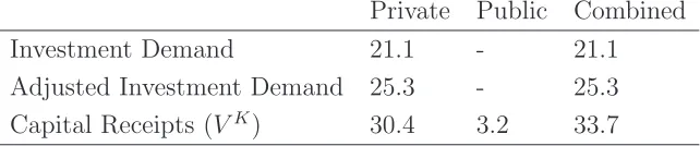
When adjusting the base year social accounts to achieve steady-state consistency, there are several degrees of freedom in the computation of an aggregate capital stock. The capital stock can be computed based upon either the capital earnings or investment. If we evaluate the capital stock on the basis of returns, with an assumed 5% interest rate and a 7% depreciation rate we find:

K0 =

VK

r+δ =

(30.4 + 3.2)

0.05 + 0.07 = 280.7

Accordingly, the steady-state investment level is calculated as:

I0 = (g+δ)K0 = 25.3

In the base-year data we find I1999 = 21.1, a value nearly 20% lower than that

implied under the steady-state assumptions. The fact that 1999 investment isbelow

3.4

Financial Capital Flows

An open economy with unrestricted borrowing is characterized by equalization of the domestic and international interest rates. In many countries, this is a coun-terfactual assumption. In the present model, we explore the role of international financial capital mobility by implementing two alternative representations of the current account constraint.

In the “Balance of Payments” model, the real exchange rate is computed within each period and adjusts to equalize the value of exports and imports in that year. That is:

X

i ¯

pX_itXit(µt) =

X

i ¯

pM_itMit(µt)

where ¯pX

it and ¯pMit are the international prices of imports and exports, Xit and Mit are the trade volumes, and µt is the real exchange rate in period t. In this model the domestic interest rate is endogenous, rD

t =µt+1/µt−1.

The “Capital Flows” model allows for net changes to the balance of payments accounts within each period. A single, infinite-horizon intertemporal budget replaces the period-by-period constraints:

∞ X t=0 X i ¯

pXitXit(µt) =

∞ X t=0 X i ¯

pMitMit(µt) = 0 (20)

and the time path of the real exchange rate is determined by the international interest rate:

µt+1 =

µt

1 +r (21)

In the open capital markets model the real exchange rate may adjust only in period 0 following a policy shock.

In the T-period model, the intertemporal trade balance is written: T X t=0 X i ¡ ¯

p_itXXit(µt)−p¯M_itMit(µt)¢

=AT+1−pK_T+1KT+1 (22)

where AT+1 is the level of terminal assets and KT+1 is the terminal capital stock,

3.5

Approximating an Infinite Horizon

Approximation of infinite horizon equilibria in this model follows the strategy pro-posed by Lau et al. [2002]. At an intuitive level, there are two issues in the ap-proximation method. First, we need to choose a terminal (period T + 1) capital stock which is consistent with smooth growth in investment in the final periods of the model (state variable targeting). Second, we need to determine an estimate of terminal assets which is consistent budget balance and steady-state growth from period T onwards. The terminal asset approximation decomposes the consumer choice problem for the infinitely-lived agent into one choice problem for periods 0 to

T, and a second problem from period T + 1 to ∞. An assumption of steady-state growth permits us to solve for period T + 1 assets using the budget constraint for the post-terminal utility maximization problem.5

Algebraically, the terminal capital stock is determined through two equations. The first is a simple capital stock evolution equation applied to the post-terminal year:

KT+1 = (1−δ)KT +IT (23) This constraint is associated with a price variable pK

T+1 which rewards investment

and depreciated capital carried over to the post-terminal year. The second con-straint selects the value ofKT+1 at a level which assures steady-state growth in the

associated control variable in the terminal period:

IT = (1 +g)IT−1 (24)

This equation replaces the zero profit condition (16) which is associated with capital stocks in the earlier periods of the model.6

5_{The determination of a reasonable value of}

T is based on numerical experimentation. We felt that for the experiments reported in this paper, a 60 year horizon provides a reasonable trade-off between run time and numerical precision. The dynamic model solves in about 5 minutes on a 1.8 GHz PC with an asset approximation error of less than 0.2%.

6_{Equation (24) represents a}

primal termination condition. An alternative approach which may sometimes provide better results is a dual termination condition, such as: pK

T+1 =

pK_T

1+r. This

In a model with international capital flows, the terminal assets of the household need not equal the value of the domestic capital stock, even if these values are equal in the initial year of the model. In order to understand our method of calculating terminal assets, it is helpful to think of the consumer utility maximization problem as two separate optimizations which are linked through the period T + 1 assets:

max PT

t=0∆tU(Ct)

s.t. A0+

PT

t=0 ¡P

ipNitNit+wtILIt +wtFLFt

¢

=PT

t=0pCt Ct+AT+1

(25)

and

max P∞

t=T+1∆tU(Ct)

s.t.

AT+1+P

∞

t=T+1 ¡P

ipNitNit+wtILIt +wtFLFt

¢

=P∞

t=T+1pCt Ct

(26)

Separability of the intertemporal utility means that when AT+1 is chosen at the

op-timal value for the ∞-horizon program, then the two subproblems together produce a consumption path which is identical to the infinite horizon program.

Suppose that T is chosen to be sufficiently long that the economy is virtually in the steady-state growth path from T + 1 onwards. In this case we can use the budget constraint from equation (26) to approximate AT+1:

AT+1 =P

∞

t=T+1 ¡P

ipCtCt−PipNitNit−wtILIt −wFt LFt

¢

≈¡

pC_TCT −PipNiTNiT −wTILIT +wTFLFT

¢1+g r−g

(27)

Using a complementarity format permits us to include this constraint in the

T-horizon model to simultaneously compute the transition path and determine the terminal asset position.7

7_{We do several calculations in the following with an equal yield public sector budget constraint.}

In these experiments, there is an immediate and permanent change in some set of taxes and we calculate the level of a replacement tax such that the present value of tax revenue over an infinite horizon remains unchanged. For these calculations we use a terminal asset equation for the public sector analogous to the household asset calculation in order to compute changes in tax revenue over the infinite-horizon, including changes induced in yearT+ 1 and thereafter:

AGT+1≈

¡

pGTGT −TTL−T K T −T

Y T −T

M T −T

vat T

¢1 +g

r−g,

4

Illustrative Applications

We present two sample applications. In the first we estimate the marginal cost of funds (MCF) under alternative model specifications. The objective of this exer-cise is develop an understanding for the relative importance of labor market and intertemporal features for the MCF. As a second sample application of the model we evaluate a seemingly beneficial proposal to reduce tariffs on High Tech/Capital intensive imports, goods which represent a large share of new investment. The log-ical appeal of such a policy is that it could promote growth through lowering the cost of capital formation. While the policy proposal seems reasonable and logical, the model reveals that the reasoning is flawed. The numerical model shows that an exemption of tariffs on this sector generates a substantial welfare loss rather than a gain. As an alternative reform, we consider the economic effect of applying a uni-form tariff and we find under a wide range of assumptions that this could provide a substantial improvement in growth and welfare.

4.1

The Marginal Cost of Funds

The marginal cost of funds is a computed value which approximates the efficiency cost of increasing public expenditure. This is computed by making a small increase in tax rates and assessing the resulting changes in tax revenue and consumer welfare. We do this calculation in the static, steady-state and dynamic models in order to evaluate the importance of the intertemporal margin. In this analysis, we compare the cost of tax revenue from each of five major revenue sources,ty, tm, vat, tl, andtk. (See Tables 3 and 4 for the rates and revenue contributions from these tax bases.)

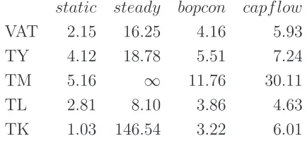
The marginal cost of funds computed in the static, steady-state, and dynamic models are listed in Tables 7, 8 and 9. We calculate the MCF as the total dollar change in Hicksian equivalent variation divided by the total dollar change in govern-ment revenues, based on model calculations in which there is a marginalproportional

increase in the tax base. In the dynamic model we use discounted present values over an infinite horizon to measure both the EV and the change in tax revenue.

which increases the distortion of a tax. This line of thought is generally consistent with the “Ramsey rule” for optimal taxation [Ramsey 1928], which suggests that taxes are more distortionary as the elasticity of demand increases.

We find that in spite of the labor market impacts, direct taxes on labor are a relatively efficient source of additional revenues. One reason this may be the case for Colombia is that existing effective taxes on labor income are low in our dataset (around 4%).

While the wage tax is relatively efficient, we find that labor market imperfections have a extremely important impact on the estimated MCF, potentially even greater than the intertemporal margin. In the current set of calculations the rigid wage model has an MCF ranging from 8 for the labor tax to infinity for the import tariff.8

What are we to conclude from these results?

1. Labor market imperfections could make public funds expensive in Colombia. A more careful assessment of the empirical evidence and appropriate theory which characterize labor markets in Colombia is required before we can assess the MCF with any degree of precision. Empirical estimation ofθ is useful and relatively easy to do.

2. A conservative lower bound on the MCF for nearly any of the tax instruments is around 1.5. This has important implications for cost-benefit analysis of public projects in Colombia.

3. MCF estimates based on the static model provide a reasonable tight lower bound on MCF estimates from a dynamic model, and MCF estimates for the steady-state model provide a loose upper bound.

8_{In the rigid-wage, steady-state model, benchmark tariff rates are on the back side of the Laffer}

curve. A marginal increase inτM _{produces a net}

Table 7: MCF Estimates from the Flexible Wage Model

static steady bopcon capf low

VAT 1.16 1.68 1.24 1.29 TY 1.57 1.78 1.48 1.51 TM 1.78 2.50 1.75 1.82 TL 1.16 1.28 1.11 1.12 TK 1.13 2.69 1.43 1.57

Table 8: MCF Estimates from the Wage Curve Model (θ = 1)

static steady bopcon capf low

VAT 1.30 2.18 1.51 1.60 TY 1.83 2.23 1.78 1.83 TM 2.08 3.38 2.19 2.32 TL 1.38 1.68 1.37 1.40 TK 1.11 3.50 1.65 1.90

Table 9: MCF Estimates from the Rigid Wage Model (θ=∞)

static steady bopcon capf low

4.2

Evaluating a Tariff Reform Proposal

A common policy goal for developing countries is increased capital formation and GDP growth. Examining Table 2, it might seem that one means of encouraging capital formation would be to lessen the tariff burden on goods which are used intensively in investment. The base year statistics indicate that capital/high tech goods (htc) comprise 29% of investment and 57% of htc supply was imported in

1999.

While the tariff rate on capital imports is only 5%, it seems (ex-ante) plausible that eliminating this tariff might expand growth. The benefits of lowering this tax must be considered in light of the costs related to raising revenues from other sources. Tariff revenues from htc imports were 0.82 billion Colombian pesos in 1999, just

over half of total tariff revenues.

When we compute the comparative dynamic growth path in the model with free capital flows, we find that eliminating the htc nearly eliminates the domestic

htc industry, particularly when the tariff is replaced by an increase in value-added

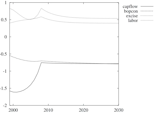
taxes. Figure 1 indicates that there a slight positive impact on investment when revenues are replaced using an excise or labor tax, but the net impact is negative when the lost tariff reveue is recovered through value-added taxes. The degree to which investment is adversely affected also depends on financial capital flows. When there is unrestricted access to international credit markets, high-technology imports are rapidly substituted for domestically produced htc goods. In the model with

period-by-period trade balance constraints, the decline of domestic htcproduction

takes place over many more years.

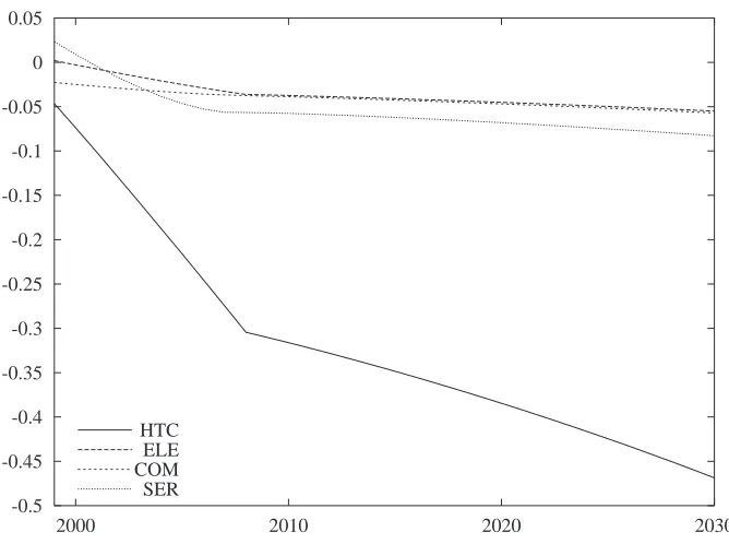
The tariff policy is shown to reduce the rate of domestic investment, but it is not completely clear why investment falls. Figure 2 helps diagnose these results. Here we have shown the absolute declines in capital demand for those sectors that experience a fall in capital use. Here we see that htc itself is responsible for the

fall in investment: htc import competition drives down the demand for domestic

htc, and this leads to a decrease in the htc demand for capital. The tariff makes

investment less expensive, but cripples the domestic industry which is most capital intensive.

labor tax could lead to an increase in investment, yet Figure 3 shows that no matter which replacement tax is applied, the tariff exemption forhtc is welfare worsening.

The least adverse impact is in the balance of payments constrained case, where the balance of payments constraint limits htcimport substitution. This implies that it

takes time for the policy to have an adverse impact.

Figure 1: Investment Response (% change)

-2 -1.5 -1 -0.5 0 0.5 1

2000 2010 2020 2030 capflow

bopcon excise labor

Policy: Permanent elimination of the tariff on

high-technology and capital-intensive goods in 1999.

Key:

capflow Unrestricted capital flows at international interest rates. (revenue replacement: VAT)

bopcon Period-by-period balance of payments con-straints and endogenous domestic interest rate. (Revenue replacement: VAT)

Figure 2: Change in Sectoral Capital Demand (%)

-0.5 -0.45 -0.4 -0.35 -0.3 -0.25 -0.2 -0.15 -0.1 -0.05 0 0.05

2000 2010 2020 2030

HTC ELE COM SER

Policy: Permanent elimination of the tariff on

high-technology and capital-intensive goods in 1999.

Key:

htc Capital and High Technology Industries ele Electricity, Gas and Water

Figure 3: Consumption Response (% change)

-0.35 -0.3 -0.25 -0.2 -0.15 -0.1 -0.05 0 0.05 0.1 0.15

2000 2010 2020 2030 capflow

bopcon excise labor

Policy: Permanent elimination of the tariff on

high-technology and capital-intensive goods in 1999.

Key:

capflow Unrestricted capital flows at international interest rates. (revenue replacement: VAT)

bopcon Period-by-period balance of payments con-straints and endogenous domestic interest rate. (Revenue replacement: VAT)

Figure 4: Consumption Response (% change)

0 0.1 0.2 0.3 0.4 0.5 0.6

2000 2010 2020 2030 capflow

bopcon

Policy: Permanent application of a uniform tariff on all

imports in 1999 at a 4% level which produces no change in government tax revenue.

Key:

capflow Unrestricted capital flows at international interest rates. bopcon Period-by-period balance of payments constraints and

5

Conclusions

We use this section to reflect on aspects of the modeling work which are not empha-sized in the paper

Data Work Substantial effort and experience were leveraged to construct and interpret the base year data for use with a CGE model. In many cases, this work is far more difficult that the actual implementation of the model equations. Although the present paper does not emphasize data issues, we caution the reader not to discount the difficulty and importance of this type of work.

Tax Interpretation The representation of tax margins in the current analysis is stylized. We have identified the key components of the direct and indirect taxes, but we have not attempted to characterize differences between the average and marginal rates nor have we considered the costs of collection or rates of evasion. Informed adjustments of the tax margins could alter the MCF estimates and could conceivably alter our policy analysis conclusions. More work is clearly warranted in this area.

Programming Details Model implementation issues have been only mentioned in the appendices describing operational details. There are a number of subtleties in-volved in the implementation of multisectoral, dynamic general equilibrium models. We rely heavily on the GAMS/MPSGE programming language for model specifica-tion (see Rutherford [1999]) and the PATH solver (see Ferris and Munson [2000]).9

Use of GAMS/MPSGE greatly reduces the scope for programming errors, as we avoid writing out cost functions, expenditure functions and demand functions. The disadvantage of the MPSGE approach is that this makes the model less accessible for economists who are unfamiliar with the syntax. It could be helpful to pro-duce an algebraic implementation of the same model using GAMS/MCP, if only to provide a transparent and comprehensive documentation of the model inputs and assumptiosn.

9_{This is not a particularly large model for PATH. The transitional dynamic model with annual}

5.1

Further Research

We can envision a number of interesting directions in which the current model might be extended. We will list some of the ideas in random order:

Taxation and violence. The present model does not address the economic ef-fects of sabotage and guerrilla activities which have severely disrupted a number of important economic activities in the country. Future application of the model might attempt to quantify the economic gains which could be realized through achieving a lasting solution to the current civil unrest.

Property rights, idle capital and growth. de Soto [2001] provides an inter-esting new perspectives on the role of property rights in the development process. Our dynamic model incorporates forward-looking markets with price-responsive in-vestment and could be calibrated to account for differences between the market and private return to capital. It could be intriguing to see if the model might be extended to quantify some of the market imperfections which DeSoto has emphasized.

International trade. The present model is based solely on national accounts for Colombia and does not incorporate bilateral trade data. It would be interesting to extend the model to provide a tool for examining the economic effects of FTAA accession or other regional trading agreements. A natural stragety for such an extension would be to build on the GTAP dataset and framework.

Tax reform and poverty. There is a 1997 SAM which provides much more sectoral and household detail. It would be quite interesting to investigate both

References

Barro, Robert J. and Xavier Sala i Martin, Economic Growth, New York: McGraw-Hill, 1995.

Blanchard, Olivier J. and Stanley Fischer,Lectures on Macroeconomics, Cam-bridge: MIT Press, 1989.

Dantzig, George B. and Alan S. Manne, “A Complementarity Algorithm for an Optimal Capital Path with Invariant Proportions,” Journal of Economic Theory, 1974,9 (3), 312–323.

de Soto, Hernando, The Mystery of Capital 2001.

Ferris, Michael C. and Todd. S. Munson, “Complementarity Problems in GAMS and the PATH Solver,” Journal of Economic Dynamics and Control, 2000, 24 (2), 165–188.

Francois, Joseph F., Bradley J. McDonald, and H. Nordstr¨om, “Capital Accumulation in Applied Trade Models,” in Richard Baldwin, ed., Dynamic issues in applied commercial policy analysis: A handbook, Cambridge University Press, 1997.

Hansen, Terje and Tjalling Koopmans, “On the Definition of Computation of a Capital Stock Invariant under Optimization,” Journal of Economic Theory, 1972, 5 (3), 487–523.

Harrison, Glenn W., Svend E. Hougaard Jensen, Lars H. Pedersen, and Thomas F. Rutherford, eds,Using Dynamic General Equilibrium Modeling for Policy Analysis, Amsterdam: North-Holland, 2000.

, Thomas F. Rutherford, and David G. Tarr, “Increased competition and completion of the market in the European Union: static and steady-state effects,” Journal of Economic Integration, 1996, 11 (3), 332–365.

Hatta, Tatsua, “A Theory of Piecemeal Policy Recommendations,” Review of Economic Studies, 1977,44 (1), 1–21.

Hutton, J. and Anna Ruocco, “Tax Reform and Employment in Europe,” In-ternational Tax and Public Finance, 1999,6, 263–288.

Lau, Morten I., Andreas Pahlke, and Thomas F. Rutherford, “Approxi-mating infinite-horizon models in a complementarity format: a primer in dy-namic general equilibrium analysis,”Journal of Economic Dynamics and Con-trol, 2002,26, 577–609.

Ramsey, Frank, “A Mathematical Theory of Saving,” Economic Journal, 1928,

38, 543–559.

Rutherford, Thomas F., “Applied General Equilibrium Modeling with MPSGE as a GAMS Subsystem: An Overview of the Modeling Framework and Syntax,”

Computational Economics, 1999,14, 1–46.

and David G. Tarr, “Regional Trading Arrangements for Chile: Do the Results Differ with a Dynamic Model?,” Working Paper, The World Bank 2001.

and , “Trade liberalization, product variety and growth in a small open economy: a quantitative assessment,” Journal of International Economics, 2002, 56, 247–272.

and Miles K. Light, “A General Equilibrium Model for Tax Policy Analysis in Colombia,” Working Paper 22, Department of National Planning 2002.

A

Running the Model

The dynamic MegaTax model is programmed in GAMS/MPSGE. The model files are organized in a directory structure, and the model is designed to run from a DOS command line. In this portion of the appendix, we describe the file structure and some built-in options for running the CGE models.

The models, data, and documentation are included in the compressed archive called dynamicmega.zip. When decompressed, this archive builds the following set of directories:

4-08-2002 10:22p <DIR> data 4-08-2002 10:22p <DIR> model 4-08-2002 10:24p <DIR> policy 4-08-2002 10:22p <DIR> mcf

The subdirectories are organized as follows:

Directory Description

data Contains original source data files (.xls for-mat) and associated data-handling routines model Contains the static and dynamic models. mcf Contains batch files, GAMS programs and

results from the calculations of the marginal cost of public funds described in section 4.1 of this paper.

policy Holds batch files, GAMS programs and re-sults from policy analysis scenarios described in section 4.2 of this paper.

We present the following sequence of tasks intended to introduce a new user to the application of the model for policy analysis. We assume that model users are familiar with a text editor which is able to read and write ASCII text files.10

A.1

Working with Existing Scenarios

A policy scenario is defined by an identifier (10 characters or less, no embedded blanks) and a set of assumed values for the model run parameters. For example, we have pre-defined a policy scenario calledutm cf, which imposes uniform tariffs in the dynamic model and assumes that international capital flows are unrestricted. Table 10 describes each of the pre-defined scenarios in the DynamicMega distribution.

Tools for making figures and tables are also included in the policy directory as

table.batand figure.bat. Using these batch files can seem awkward at first, but they offer a structured approach for managing policy scenarios.

A.1.1 Creating Tables

table.gms is a GAMS program designed to produce tables which compare two or more scenarios, side by side. Commonly-used output parameters have already been defined in table.gms, such as output, international trade and consumption.

table.gms is called from the table.bat control program. The main idea behind using batch files is to allow a command-line interface for GAMS, where scenario choices can be easily changed and viewed.

Syntax:

table.bat {output parameter} {scenario1 [scenario2. . . ] }

Output Parameters: Currently, there are four output parameters for use withtable.gms. Additional output parameters can be included directly into the table.gms file.

table.gms Pre-defined Output Parameters:

10_{Three text editors are included with Windows, including Notepad, Wordpad and Edit. We feel}

Table 10: Presolved Policy Scenarios

Identifier Description

utm cf policy=utm horizon=capflow

Uniform tariffs in the dynamic model with unrestricted capital flows (open capital markets).

utm bp policy=utm horizon=bopcon

Uniform tariffs in the dynamic model with period-by-period balance of payments constraints (closed capital markets).

utm st policy=utm horizon=static

Uniform tariffs in the static model

utm ss policy=utm horizon=steady

Uniform tariffs in the steady-state model

htx cf policy=utm horizon=capflow

Free trade in high tech goods in the dynamic model with unrestricted capital flows (open capital mar-kets).

htx bp policy=exempt horizon=bopcon

Free trade in high tech goods in the dynamic model with period-by-period balance of payments con-straints (closed capital markets).

htx st policy=exempt horizon=static

Free trade in high tech goods in the static model

htx ss policy=exempt horizon=steady

output Sectoral Production (% change)

import Imports by sector (% change)

export Exports by sector (% change)

results Summary results for several key economic metrics, such as Equivalent Variation, Formal and Informal Wages, and Return to Capital

How data flows between batch files and GAMS programs is initially confusing. The typical structure for making a table across scenarios is shown in the diagram below.

table.bat and Related Files

table.bat [ Scenario 1 ... 6 ]

| [ Output parameter choice ]

|

table.inc Small include file which gets read by

| table.gms

| table.gms

| | | |

---| | | |

table.lst table.txt table.tex screen output

Example: Import Comparisons

As an example, we compare the change in imports for Colombia across two tariff reform scenarios: ss utmand st utm. First, connect with the policy sub-directory in the DynamicMega distribution, then execute the following command:

c:\model\policy>table.bat import ss_utm st_utm

This callstable.batfrom thepolicydirectory, which passes the output parameter and the scenarios to table.gms. The table is printed in three ways: to the screen for quick viewing, to a text file, and to a file which can be read by LA

TEX. The text version of the corresponding output table is:

Imports (% change)

---st_utm ss_utm

---CRO 71.1 72.9

LVS -23.1 -22.4

FFH -2.9 -2.4

OIL -31.0 -31.0

MIN -11.8 -10.2

FOD 13.4 12.5

NRI 0.6 1.8

NSI -0.5 -1.4

HTC -0.2 -0.1

TRN -30.3 -31.0

ELE -32.0 -34.1

COM -30.8 -33.8

SER -29.2 -30.8

---A.1.2 Creating Figures

Pre-defined Plotting Parameters for use with figure.gms:

pctev Percentage equivalent variation wage f Formal wage

wage i Informal wage

rent Rental rate for capital rexch Real exchange rate lsup f Labor supply – formal lsup i Labor supply – informal pctinv Investment

capital Capital stock consum Consumption

The file structure for figure.bat is similar to table.bat. Data flows through the following files:

figure.bat and Related Files

figure.bat [ Scenario 1,2,.. (up to 6) ]

| [ Output parameter choice ]

|

figure.inc Small include file which gets read by

| figure.gms

|

figure.gms Passes data to GnuPlot for plotting

| [gp_opt Options can be included for fine-tuning]

|

gnuplot Produce the plot

| |

plot Resulting figure, to the screen or

to an output file (.gif or .eps)

Example: Role of Capital Flows

A new figure is created by calling figure.bat with options which choose the sce-narios and output parameter:

This command plots the percentage change in investment for two scenarios: uniform tariffs with closed capital markets, and uniform tariffs with open capital markets. The resulting plot is shown in Figure 5.

Figure 5: Scenario Comparison Using figure.bat

0.4 0.6 0.8 1 1.2 1.4 1.6 1.8 2 2.2 2.4

2000 2010 2020 2030

bp_utm cf_utm

A.2

Defining New Scenarios

Inevitably, new scenarios will be needed as new policy decisions arise. A new set of scenarios can be created created by changing the default $setglobal (input) variables and giving the scenario a name. All of the pre-defined $setglobal input choices are listed in Table 11. When adding new sets of scenarios, we recommend copying thepolicy directory and renaming it according to the new set of scenarios. These new scenarios are created for new policy considerations, or to conduct sensi-tivity analysis for existing policies. As an example, we compare the uniform tariff experiment across different elasticity choices.

Example: Change Existing $setglobals

Table 11: Model Input Parameters for the Static and Dynamic MEGA Models

Variable Default Description

policy blank Trade policy option: utmfor uniform tariff or exempt

for tariff exemptions applied to capital-intensive and high-tech goods.

horizon static Model time horizon, one of four options: static,

steady, bopcon, and capflow. The bopcon formula-tion is based on the dynamic model with closed cap-ital markets (balance of payments constraints), and

capflowis based on the dynamic model

LabMarket HT Labor market formulation. HT refers to the Harris-Todaro model with unit elasticity wage-unemployment curve in the formal sector. HTU de-scribes Harris-Todaro with a fixed formal sector wage and classical unemployment, Flexible refers to a neoclassical labor market with flexible wages and fixed supply of both formal and informal labor.

etrndx 2 Output elasticity of transformation between domestic and export markets.

esubt 0.5 Intertemporal elasticity of substitution.

esubdm 4 Armington elasticity between domestic and imported goods.

scenario files from policy into the new directory. This is done from the command prompt, in the top-level (model) directory.

c:\model>mkdir sensitivity

c:\model>copy policy\*.* sensitivity

Now, edit the batch file called: solves.batto define a new set of scenarios to solve. Delete the old SOLVE statements and consider the following solves:

CALL SOLVE arm_low_st esubdm=0.5 u_tm=yes horizon=static CALL SOLVE arm_med_st esubdm=8 u_tm=yes horizon=static CALL SOLVE arm_hi_st esubdm=16 u_tm=yes horizon=static

CALL SOLVE ht_off u_tm=yes horizon=static ht=no

CALL SOLVE ht_on u_tm=yes horizon=static

Notice that all of the scenario names are less-than 10 elements. Longer names will cause an error in GAMS.

With the newly defined scenarios, we can simply call the solve.bat command file and run all of the scenarios:

c:\model\sensitivity>solves.bat

Once the scenarios have been solved, we make a table to quickly compare the results:

c:\model\sensitivity>table.bat results arm_low_st arm_med_st arm_hi_st ht_off ht_on

The resulting table (in LA_{TEXformat) looks like this:}

Summary results

arm low st arm med st arm hi st ht off ht on

REXCH 0.1 0.2 0.4 0.1 0.2

PCTEV 0.0 0.3 0.8 0.3 0.3

RENT 0.0 1.0 2.2 0.9 1.0

LSUP F 0.0 0.5 1.1 0.3 0.5

LSUP I 0.0 -0.7 -1.6 -0.5 -0.7

WAGE F 0.0 0.0 0.1 0.2 0.0

It is clear from the senstivity analysis that the Armington elasticity of substitution between domestic and imported goods will drive welfare and labor results. We also see that migration and unemployment are less important when considering tariff reform in the static framework than in the steady-state model.

Example 2: Change the default model. This example shows you how to change the default model specification, then re-run all of the given scenarios. This makes use of the model.gms file included in the policy directory. The model.gms file defines all of the available setglobals for a given scenario folder. For example, the

sensitivityfolder contains the following model.gms file:

model.gms:

$if not setglobal horizon $setglobal horizon static $if not setglobal u_tm $setglobal u_tm no

$if not setglobal htft $setglobal htft no

$if not setglobal ht $setglobal ht yes $if not setglobal theta $setglobal theta 1

$if not setglobal esubt $setglobal esubt 0.5 $if not setglobal etrndx $setglobal etrndx 4 $if not setglobal esubdm $setglobal esubdm 8 $if not setglobal esubkl $setglobal esubkl 1

$if %horizon%==capflow $include ..\model\dynamic $if %horizon%==bopcon $include ..\model\dynamic $if %horizon%==static $include ..\model\static $if %horizon%==steady $include ..\model\static

$if %horizon%==capflow $include dynamic-scenarios.gms $if %horizon%==bopcon $include dynamic-scenarios.gms $if %horizon%==static $include static-scenarios.gms $if %horizon%==steady $include static-scenarios.gms

The default values for each input variable is set at the top. The bottom sec-tion simply directs the solver to the relevant GAMS model. For example, if the

For example, change the default wage-curve elasticity to a low number inmodel.gms:

$if not setglobal theta $setglobal theta 0.2

Now, empty the output directory and resolve all of the cases:11

c:\model\sensitivity>del output\* c:\model\sensitivity>solves.bat

Now check to see if the Harris-Todaro formulation has a more dramatic impact under the Uniform Tariff reform by calling thetable.bat command for each of the scenarios. The corresponding table for this model is:

A.3

Create a New

$setglobal

Option

Global variables can be created anytime a new type of model control is needed. Initially, it may seem that global variables are un-necessary to control model inputs. It would be easier for the modeler to simply enter the new input values into the model file by hand. Directly changing parameter values or model structure is fine for small problems and simple counterfactual analysis, but this approach soon becomes unwieldly. Common errors (by at least one of the authors) include forgetting to reset a switch when producing different figures, or acidentally re-setting a parameter before reporting it.

When a new policy variable is needed, create it using a $setglobal variable, which includes a default value. In this way, counterfactual scenarios can be traced back to the model.gmsfile or thescenariofile used to generate it. The extra effort of using a $setglobal is rewarded with consistent scenario management.12

Example: Develop a uniform VAT switch

As an exercise, we will consider uniform value-added taxes in the static, steady-state, and dynamic models. We will define a $setglobal variable which equalizes

11_{Deleting the existing solution files is important. The batch files check for existing solves with}

the same name. If an identical .solalready exists, then the program skips that scenario to save time.

12_{For a detailed discussion of scenario management see the discussion by Rutherford included in}

allvat rates, calledu vat. Whenu vatis true, then each VAT rate is equalized, and the VAT tax multiplier, τvat, is allowed to adjust to hold government expenditures constant.

First, we must create a new scenario directory, then copy the policy files into the new directory.

c:\model>mkdir uvat

c:\model>copy policy\*.* uvat

We don’t need to copy the output directory over because it will be automatically created when a new scenario is run. In this case, it is easiest to include the global variable into the dynamic and static scenario files. At the top of the file, add a statement such as:

if (%u_vat%,

vat(s) = sum(ss, vat(ss) * a0(ss)) / sum(ss, a0(ss)); replace("vat") = yes;

);

With the new $setglobal variable in place, we can now use solves.bat to execute a set of new scenarios. Edit the solves.bat file, renaming the uniform tariff scenarios to uniform VAT:

CALL SOLVE cf_utm horizon=capflow u_tm=yes CALL SOLVE bp_utm horizon=bopcon u_tm=yes CALL SOLVE st_utm horizon=static u_tm=yes CALL SOLVE ss_utm horizon=steady u_tm=yes

CALL SOLVE cf_uvat horizon=capflow u_vat=yes CALL SOLVE bp_uvat horizon=bopcon u_vat=yes CALL SOLVE st_uvat horizon=static u_vat=yes CALL SOLVE ss_uvat horizon=steady u_vat=yes

After calling solves.bat from the command line, we can generate some tables and plots for these scenarios. First, we generate a table to compare consumption and investment across time-frames.

Table 12: Summary Results for Uniform Tariff Scenarios

ss uvat st uvat bp uvat cf uvat PCTEV 0.3 0.1 0.3 0.3 WAGE F 0.2 0.0 0.1 0.1 WAGE I 0.2 -0.1 0.2 0.1 RENT 0.8 1.1 0.8 1.0 REXCH -0.1 -0.3 0.0 -0.2 LSUP F 0.9 0.7 0.5 0.5 LSUP I -1.3 -1.2 -0.6 -0.8

As expected, we see that the benefits of a uniform VAT are bounded below by the static model results and above by the steady-state model results. We can also plot the transition path between the short-run impact and the new steady-state using the figure routine:

c:\model>figure.bat consumption bp_uvat cf_uvat

Of course, it is impossible to plot items from the static and steady-state scenario runs because they are comparative-static outputs. The transition path for u vat

under the free-capital markets and balance-of-payments constraint assumptions is shown in Figure 6. Finally, we compare the welfare gains over time for a uniform tariff and uniform VAT:

c:\model>figure.bat consum cf_utm cf_uvat

We find that the welfare benefits of tariff uniformity are greater than those for a uniform VAT. Of course, these figures do not include institutional costs such as the cost of collection and the propensity for tax evasion.

A.4

The Scenario Manager

Figure 6: Welfare Change for Uniform VAT Tax Reform

0.05 0.1 0.15 0.2 0.25 0.3 0.35

2000 2010 2020 2030

percent change

Consumption

capflow bopcon

Figure 7: Comparison of Uniform VAT vs. Uniform Tariffs

0.2 0.25 0.3 0.35 0.4 0.45 0.5

2000 2010 2020 2030

percent change

Consumption

contains only one or two relevant policy experiments. Decision-makers are different. They will often ask for several policy alternatives to help them frame a given policy debate and come to a reasonable decision. For these people, we recommend using the Scenario Manager (SM). This tool is a stand-alone program which can run on any Windows-based personal computer. The main advantage of the Scenario Manager is that the existing scenarios can be included into the SM with relatively little effort. Documentation and theology regarding this tool is available on the GAMS homepage in the MPSGE section.

A.5

File Listing

Table 13: Itemized File Description for DynamicMega

data folder:

build.bat Batch file which calls makedata to generate a balanced SAM for 1996 and 1999.

makedata.bat Batch file which callssam99orsam96for data balancing.

balance.gms A program used to balance the 1996 and 1999 Colom-bian SAMs. This program uses an NLP approach to balance the National Accounts.

sam9X.gms sam9X.dat sam9X.xls

The .xls files are original datasets from Sergio Prada. The.gmsfiles import the XL data into GAMS and write the .dat files for inclusion into GAMS.

balanced99.dat balanced96.dat

Balanced datasets used in the MPSGE models. This data is included in thedata.gms program in the model directory.

model folder:

data.gms Organizes the Colombian SAM data for inclusion into the MPSGE model. Data is mapped onto sectoral de-mand and output. Tax revenues and transfers are cal-culated and parameterized. Basically all of the data handling is completed in this file.

static.gms Static and Steady-State MPSGE formulation for Colom-bian economy. Uses data.gms for data-handling and preperation.

dynamic.gms Multi-sectoral dynamic CGE model for Colombia. Uses the same data handling file as the static model: