A Novel Evolutionary Algorithm with Neighborhood Search for Project Portfolios Optimization Problem

http://dx.doi.org/10.4236/ajibm.2015.56040

How to cite this paper: Lei, W.D. and Li, S.K. (2015) A Novel Evolutionary Algorithm with Neighborhood Search for Project Portfolios Optimization Problem. American Journal of Industrial and Business Management, 5, 396-403.

http://dx.doi.org/10.4236/ajibm.2015.56040

A Novel Evolutionary Algorithm with

Neighborhood Search for Project Portfolios

Optimization Problem

Weidong Lei, Suike Li

School of Management, Northwestern Polytechnical University, Xi’an, China Email: [email protected], *[email protected]

Received 28 May 2015; accepted 23 June 2015; published 26 June 2015

Copyright © 2015 by authors and Scientific Research Publishing Inc.

This work is licensed under the Creative Commons Attribution International License (CC BY).

http://creativecommons.org/licenses/by/4.0/

Abstract

This paper proposes a quantum-inspired evolutionary algorithm with neighborhood search (call- ed QEANS) to solve the project portfolios optimization problem with limited multiple resources and bounded risks for each project portfolio. The decision concerns how to find an optimal or best assignment of projects to a set of project portfolios that maximizes the total profit. The studied problem is formulated by a 0-1 linear programming model, and a quantum-inspired evolutionary algorithm with neighborhood search is proposed to solve it. In specific, each problem solution is encoded by a Q-bits matrix, which is updated by quantum-rotation gate. In addition, crossover and mutation operators are integrated so as to increase the population diversity. Furthermore, an ef-fective repairing procedure is proposed for dealing with the generated infeasible solutions. To prevent the local optimum, a specific neighborhood search procedure is also proposed. Randomly generated instances are used to test and justify the effectiveness of the proposed QEANS. The ob-tained results indicate that the proposed QEANS is effective.

Keywords

Project Portfolio, Optimization, 0-1 Linear Programming, Quantum Evolutionary Algorithm

1. Introduction

them may be quickly transformed into new products (services) or new technologies, which are then widely spread across the world. Due to this reason, new markets or services will be created and new companies or en-terprises are founded. Therefore, all companies have to compete with each other and suffer from uncertain oper-ational risks as well as relatively small profit margins. Hence, almost all the great or powerful enterprises adopt the market diversification strategy and expect to mitigate risks, improve competitiveness, maintain company’s sustainability and obtain considerable profits from different marketing fields.

In practice, only minority companies had achieved their expectations and most of them had failed. The rea-sons were generally from two aspects. One aspect was that companies had made wrong market diversification strategies because of many reasons, so company’s resources (i.e., money, technologies, human resources and so on) were used in wrong places and wasted. The other was that companies had made proper diversification strat-egies but they lacked sufficient ability or resources to implement them, because the diversification strategy gen-erally belonged to macroscopical level, and it must be reflected in the specific business activities. From this point, we can know how to choose specific business activities from numerous possible ones for achieving com-pany’s long-term strategy and how to assign existing limited resources to each chosen activity as well as how to manage them to effectively play a key role in the success of strategy implementation.

To tackle the above mentioned problems, it is a good choice to implement the diversification strategy by us-ing the methodology of Project Portfolio Management (PPM). Accordus-ing to [1] and [2], project portfolio man-agement refers to the process for effectively identifying, assessing, selection, and optimizing the collection of projects in order to meet some certain expectations and needs (such as long-term strategic objectives) of an en-terprise or a company. From above descriptions, we can know that company’s strategy implementation can be seen as project management process, as company’s new businesses can be seen as projects, and project portfolio management is an important tool to effectively manage and implement these projects in strategy implementation. A key issue to the project portfolio management is the portfolio selection and resource allocation problem.

Motivated by the above descriptions, this paper proposes a novel meta-heuristic approach (called Quantum- inspired Evolutionary Algorithm with Neighborhood Search, QEANS) to solve the strategy-oriented project portfolio optimization problem under bounded risks and with the consideration of resources sharing in different projects. This problem is NP-complete. Our objective is to find an optimal projects selection scheme such that the overall revenues of selected projects are maximized.

The rest of this paper is arranged as follows. Section 2 presents the literature review. The problem description and its formulation are given in Section 3. In Section 4, we introduce the proposed solution method, i.e., Quan-tum-inspired Evolutionary Algorithm with Neighborhood Search (QEANS). In Section 5, randomly generated instances are used to test the effectiveness of the proposed algorithm. At last, Section 6 concludes this paper and discusses some possible future research directions.

2. Literature Review

This section presents a literature review of related project portfolio problems and Quantum-inspired Evolutio-nary Algorithm (QEA). Studies on different kinds of project portfolio problems have been reported by research-ers. For example, Arcjer and Ghasemzadeh [3] developed a decision support system consisted by a multi-stage integrated framework for the project portfolio selection process. Dickinson et al. [4] proposed a nonlinear integ-er program model for optimizing the portfolio of new technology projects selection problem with considinteg-ering the interdependencies between different projects. Girotra et al. [5] investigated the structure and effect of mul-tiple projects targeting the same market at the portfolio level. Chen and Askin [6] developed a general mathe-matical formulation for the joint problem of selecting and scheduling projects with maximizing the present worth of profit. Besides, Coffin and Taylor [7] developed a beam search procedure for solving the R&D projects selection and scheduling problem. Heidenberger [8] developed an MILP (mixed integer linear programming) approach for dynamic projects selection problem. In addition, some researchers also proposed effective ap-proaches for the projects selection problem from very specific background. For instance, Badri et al. [9] formu-lated a 0 - 1 goal programming model for IS (Information System) project selection problem. Eilat et al. [10] developed a DEA (Data Envelopment Analysis) model embedded in the BSC (Balanced Score Card) approach for funding suitable projects from new R&D portfolios.

parallelism and quantum updating gate. It has showed very good performance in terms of solution quality and computation time in solving many famous combinatorial optimization problems. For instance, Narayanan and Moore [12] and Talbi et al. [13] proposed different QEAs to optimize the travelling salesman problem (TSP) and obtained better performance compared to traditional approaches. Han and Kim [14] and Zhao et al. [15] de-veloped various effective QEAs for knapsack problems. Besides, some researchers have also dede-veloped different kinds of QEA for flowshop/jobshop scheduling problem [16] [17].

Viewing from the above descriptions, we can see that project portfolio optimization problem with limited risks and multiple kinds of resources have rarely been studied in the literature. In addition, various efficient QEAs have been applied in several research fields except for optimizing project portfolio problem. Therefore, this work tries to connect this research gap.

3. Problem Description, Notation and Formulation

3.1. Problem Description

In this paper, we consider the following problem. Suppose that a company decides to use the methodology of project portfolio management to achieve its strategic objectives. And according to its strategic objectives, the company intends to invest some idle resources (including money, technology, human resource and so on) to N new projects which had been evaluated by professional experts and are considered to have great investment val-ue, that is, the success of implementing these new projects can effectively help the company improve its compe-titiveness, maintain high sustainability, maximize its incomes and so on. Here, we suppose that all resources quired for implementing these new projects are available or the company has the ability to get the required re-sources for carrying out these new projects. Furthermore, it is supposed that each project has its own expected revenue and potential risk of failure. We also suppose that some different projects may use the same type of re-sources (such as technology or equipment), which is called resource-sharing. Besides, due to resource limita-tions, the company can only implement at most M project portfolios at a certain period of time, that is to say, each project portfolio has a maximum resource allocation quantity. In order to control risk in an acceptable range or level, each project portfolio must have a maximum risk tolerance. That is to say, the overall risks of projects belonging to a same project portfolio cannot exceed the pre-defined maximum risk setting.

Based on the above descriptions, this paper studies how to optimize the project portfolio selection problem with satisfaction of bounded portfolio-risks and resource limitations. The decision concerns how to select the projects among a given set of projects for each project portfolio such that the total profits of selected projects in all portfo-lios are maximized. To facilitate the problem formulation, we give the following notation and decision variables:

N: the number of total projects. M: the number of project portfolios. K: the types of available resources.

Rj: the maximum risk acceptance degree of project portfolio j, 1 ≤j ≤M. vi: the expected revenue or profit of project i, 1 ≤i ≤N.

ri: the failure risk of project i, 1 ≤i ≤N.

Ck, j: the maximum quantity of resource k assigned to project portfolio j, 1 ≤k ≤K, 1 ≤j ≤M. qk, i: the quantity of resource k assigned to project i, 1 ≤i ≤N, 1 ≤k ≤K.

ϕk: the sharing-degree of resource k, and ϕk∈ [0, 1], 1 ≤k ≤K. If ϕk = 0, it means that resource k cannot be shared or used by different projects; Otherwise, resource k (such as equipment and buildings) can be completely used by different projects.

µ_i: the projects similarity of project portfolio i, and µ_i∈ (0, 1), 1 ≤i ≤M. For µ_i≈ 0, it implies that all projects in portfolio i are different, and for µi≈ 1, it implies that all projects in portfolio i are nearly the same ones. It should be noted that, since there does not exit the same projects, we have µi≠ 1.

The decision variables are the following: V: the total profits of M project portfolios.

xi, j: 0-1 variable. If xi, j = 1, it means that project i belongs to project portfolio j; Otherwise (i.e., xi, j = 0), project i does not belong to project portfolio j, for 1 ≤i ≤N, 1 ≤j ≤M.

3.2. Mathematical Model

prob-lem with limited resources and bounded risks can be formulated as follows:

, 1 1

Max M N i i j

j i

V v x

= =

=

∑∑

subject to:

,

1 1, for 1 ,

M i j

j= x i N

≤ ≤ ≤

∑

, 1

, , , ,

1 , for 1 , 1

N

k j i j

N

i

k i i j k j k j

i

x

q x C C k K j M

N ϕ µ

=

=

−

∑

∑

, 1 ,

1 1 2 , for 1

N i j N

i

i i j j j

i j

x

r x R R j M

N µ = =   +_ − _∗ ∗ ≤ ≤ ≤  

∑

∑

In the above model, the problem objective is formulated as (1), i.e., maximization of the total profit of all portfolios. Constraint (2) indicates that each project i can only be assigned to at most one project portfolio j, be-cause it cannot be divided. From this definition, we can know that each project is either be selected for a project portfolio or not be selected. Furthermore, constraint (3) defines that the total resource of type k required by all projects in a portfolio j cannot exceed its pre-allocated quantity Ck, j. Finally, constraint (4) defines that the over-all risk of over-all projects in a project portfolio j cannot exceed its pre-defined maximum risk acceptance level Rj.

4. Solution Method

In this section, due to the NP-complete characteristic of our studied problem, we introduce a novel meta-heuris- tic approach to solve it. That is called as Quantum-inspired evolutionary algorithm (QEA) with neighborhood search procedure. In what follows, we first introduce the Q-bits representation, and then describe other compo-nents of the proposed algorithm in details.

4.1. Representation

QEA is formulated according to the principles of quantum computing [11] [14]. The smallest unit of information in QEA is called Q-bit, which is usually defined as follows [14]:

2 2

0 1 , where 1

ψ =α +β α + β = . (5)

In Equation (5), complex numbers α and β respectively denote the probability amplitudes of Q-bit ψ in state “0” and state “1”. From this definition, we can know that each Q-bit would be found in state “0” with probabili-ty |α|2 _{or in state “1” with probability |β|}2_{. In order to determine its final state, a random-key observation way is}

generally applied to each Q-bit. In specific, a number rd is randomly generated from uniform distribution [0, 1). If rd > |α|2_{, then Q-bit is in state “1”; otherwise, Q-bit is in state “0”. Due to this reason, QEA can be regarded as}

a probabilistic algorithm.

As mentioned above, the value of integer decision variable xi, j belongs to 0 or 1. Hence, it has a same charac-teristic with Q-bit. Inspired by this fact, the chromosome is defined as follows:

1,1 1,2 1,

2,1 2,2 2,

,1 ,2 ,

M

M N M

N N N M

ψ ψ ψ

ψ ψ ψ

ψ ψ ψ

×       Ψ =         , where 2 2

, , 0 , 1 , and , , 1, for 1 , 1

i j i j i j i j i j i N j M

By using the above mentioned random-key way, the final state of each Q-bit ψi, j can be determined. If Q-bit ψi, j is in state “0”, we let it represent that project i is not in portfolio j, i.e., xi, j = 0; Otherwise, project i is in portfolio j, i.e., xi, j = 1. Finally, all values of decision variables xi, j (hereafter we called binary matrix X) are known, and correspondingly, the objective value (i.e., V) can also be calculated.

4.2. Feasibility Checking Procedure

For each obtained binary matrix X (i.e., values of decision variables xi, j) associated with a Q-bits chromosome, it may be an infeasible solution. Therefore, we need to check whether it satisfies the problem constraints (2), (3) and (4). If it does not satisfy the problem constraints, then we repair it. To do this, consider the following:

Step (A): Check constraint (2). Because each project can only be assigned to at most one project portfolio, for any project i (1 ≤i ≤N), if it is assigned to more than one project portfolio, we randomly remove it from one of portfolios (i.e., reset xi, j = 0, 1 ≤j ≤M), until constraint (2) is satisfied.

Step (B): Check constraint (3). Suppose that maximum resource (type k) quantity of project portfolio j (i.e., Ck,

j) is exceeded, then we remove project i with the minimum ratio value of vi/qk, i from project portfolio j until the total required resources of projects in portfolio j are smaller than or equal to Ck, j.

Step (C): Check constraint (4). Suppose that the maximum risk acceptance degree (i.e., Rj) of portfolio j is exceeded, then we remove project i with the minimum ratio value of vi /ri from project portfolio j until the over-all risk of portfolio j is satisfied.

Based on the above works, each obtained problem solution (i.e., binary matrix X) is either proved or repaired to be feasible. Hence, the corresponding objective value can be easily calculated.

4.3. Updating Q-Bits Individuals

For each Q-bit ψi, j in a quantum chromosome Y, it is updated by the well-known quantum rotation gate, which is usually defined as the follows [14]:

(

)

(

)

(

)

(

)

, , , , ,

, , , , ,

cos sin

sin cos

i j i j i j i j i j

i j i j i j i j i j

α α θ β θ

β α θ β θ

′ = × ∆ − × ∆

′ = × ∆ + × ∆ for 1≤ ≤i N,1≤ ≤j M. (7)

In (7), ∆θi, jis the rotation angle, which decides the rotation direction and magnitude in the process of updat-ing Q-bit ψi, j. We first define θ0 be the initial rotation angle, and then suppose that VY represents the objective value related to quantum chromosome Y, and VB represents the objective value of the best chromosome (denoted by B) found in population. Similar to [14], the rotation angle ∆θi, jis determined based on the values of decision variable xi, j in individual Y (marked as Y-xi, j) and in the best one (marked as B-xi, j). If VY < VB, then consider the following cases:

(a) For Q-bit ψi, j in the 1st or 3rd quadrant, if Y-xi, j = 1 and B-xi, j = 0, then we set ∆θi, j = θ0, which aims to

in-crease the probability of Q-bit ψi, j in state “0”; else if Y-xi, j = 0 and B-xi, j = 1, then we set ∆θi, j = (−θ0), which

aims to increase the probability of Q-bit ψi, j in state “1”; else, ∆θi, j = ±0.002π, which aims to let Q-bit search its neighborhood area.

(b) For Q-bit ψi, j in the 2nd or 4th quadrant, if Y-xi, j = 1 and B-xi, j = 0, then we set ∆θi, j = (−θ0), which aims to

increase the probability of Q-bit ψi, j in state “0”; else if Y-xi, j = 0 and B-xi, j = 1, then we set ∆θi, j = θ0, which

aims to increase the probability of Q-bit ψ_{i, j} in state “1”; else, ∆θ_{i, j} = ±0.002π, which aims to let Q-bit search its neighborhood area.

4.4. Chromosome Mutation

To increase the population diversity, mutation operation is applied to quantum chromosome according to certain probability. In particular, four points p, q, g, h (they can be the same or different) are randomly generated for each chosen chromosome, 1 < p, q < N, 1 < g, h < M, then, for each Q-bit ψi, j, p≤i≤q, g≤j≤h, we swap its amplitudes of states “0” and “1”, that is, the original Q-bit ψi, j is defined as: |ψi, j〉 = α i, j|0〉+β i, j|1〉, after muta-tion operamuta-tion, it becomes: |ψi, j〉 = βi, j|0〉+α i, j|1〉.

4.5. Binary Matrix Variation

solutions (i.e., values of decision variable xi, j) according to their respective probabilities. In specific, binary tournament method is used to select individuals for crossover. At first, four different points p, q, g, h are ran-domly generated, 1 < p, q < N, 1 < g, h < M. For generating offspring1, the value of xi, j (p ≤i ≤q, g ≤j ≤h) is copied from parent 2, and the values of other xi, j (i ∉ [p, q], j ∉ [g, h]) is copied from parent 1; similarly, for offspring2, the value of xi, j (p ≤i ≤q, g ≤j ≤h) is copied from parent 1, and values of other xi, j (i ∉ [p, q], j ∉ [g, h]) is copied from parent 2.

Furthermore, mutation operator is applied to each chosen problem solution X. More precisely, four different points p, q, g, h are randomly generated, 1 < p, q < N, 1 < g, h < M. For p ≤i ≤q, g ≤j ≤h, if xi, j in X is equal to 1 (i.e., project i is in project portfolio j), then we set xi, j = 0; else (i.e., project i is not in project portfolio j), then we set xi, j = 1.

4.6. Neighborhood Search Procedure

For improving the solution quality as many as possible, neighborhood search procedure is applied to the ob-tained binary matrix at each generation. In specific, for a binary matrix X, if there exists a project i which does not be assigned for any of project portfolios (i.e., for each j, we have xi, j = 0), then we randomly put it into project portfolio j (1 ≤j ≤M), i.e., setting xi, j = 1; else, if project i is in project portfolio j (i.e., xi, j = 1), then we randomly put it into project portfolio j − 1 or j + 1 (i.e., setting xi, j = 0 and xi, j−1 = 1 or xi, j+1 = 1). Finally,

eva-luate all the generated new solutions, and update the best solution.

4.7. Quantum Population Re-Initialization

Although several effective variation ways have been proposed to increase the diversity of quantum population and problem solutions, it still has some possibilities to enhance the diversity in order to prevent the algorithm falling into the local optimum. To do this, we re-initialize all the quantum chromosomes at every λgeneration.

4.8. Steps of the Proposed Algorithm

Input: Pops (size of the quantum chromosomes); Maxgen (maximum number of iterations); cp (crossover proba-bility); mp (mutation probability); λ(population re-initialization period); θ0 (the initial rotation angle).

Output: the best solution VBand xi, j.

Step (I): Randomly initialize quantum chromosomes and set t = 0.

Step (II): Determine Q-bits state, and assign the corresponding value to decision variable xi, j. Step (III): Evaluate individuals, i.e., check the feasibility of the obtained solutions xi, j. Step (IV): Store the best solution among all the solutions and related values of variables xi, j. Step (V): Let t = t + 1.

Step (VI): if t > Maxgen, then go to stop and output the stored best solution; else, go to Step (VII). Step (VII): Apply Q-gate to update each quantum chromosome.

Step (VIII): Apply mutation operator to quantum chromosomes.

Step (IX): Determine Q-bits state, evaluate individuals, and finally update the best solution. Step (X): Apply crossover and mutation operators to obtained binary matrixes (i.e., xi, j). Step (XI): Evaluate individuals and update the best solution.

Step (XII): Apply neighborhood search procedure.

Step (XIII): At every λ generation, re-initialize all the quantum chromosomes. Then, determine the Q-bits state, evaluate individuals, and finally update the best solution .After that, go to Step (V).

5. Computational Results

0.9); the maximum risk acceptance level of project portfolio j is set as: Rj = U (0.85, 1), for 1 ≤j ≤M. Moreover, the sharing-degree of resource k is set as ϕk = U (0.1, 0.95), for 1 ≤k ≤K. For each given values of N, M and K, five instances are randomly generated. Furthermore, the algorithm parameters are set as follows: Maximum generations: Maxgen = 500; Population size: Pops = 500; Crossover probability: cp = 0.8; Mutation probability: mp = 0.1; Population re-initialization period: λ= 20.

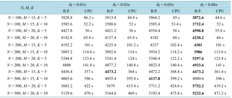
Table 1 reports the computational results on the randomly generated instances. Note that the “B.P.” and the “CPU” respectively refer to the average best profit and the average computation time of the five randomly gen-erated instances (for each given values of N, M and K). Since the rotation angle (i.e., θ₀) has positive effect to the performance of QEANS, we set θ₀∈ {0.01π, 0.03π, 0.05π, 0.08π} in our experimental study to further test its influence to the algorithm. From Table 1, we can see that both the average total profit (i.e., B.P.) and the CPU time (i.e., CPU) increase with the problem size (i.e., the value of N and M). We also notice that the CPU times gaps of different rotation angle settings for each given value of N, M and K are generally small and in the range of 0 s - 6 s, which can be neglected. Besides, we can also see from Table 1that our proposed QEANS with θ₀ = 0.08π has a better performance than that with other rotation-angle settings, for almost all the tested in-stances except for the one with setting N = 500, M = 15 and K = 10. Moreover, for random instance with N = 500, M = 15 and K = 5, our algorithm with θ₀ = 0.03π has a better solution quality than that with θ₀ = 0.08π, please see the bold font in Table 1. Figure 1 illustrated the results curves of different parameter settings. From above descriptions, we can conclude that our proposed QEANS is effective for solving the studied optimization problem in terms of solution quality and computation time.

Figure 1. Best solutions obtained with our proposed QEANS with different parameter settings.

Table 1. Computational result on random instances with θ0∈ {0.01π, 0.03π, 0.05π, 0.08π}.

N, M, K θ0 = 0.01π θ0 = 0.03π θ0 = 0.05π θ0 = 0.08π

B.P. CPU B.P. CPU B.P. CPU B.P. CPU

N = 100, M = 15, K = 5 3828.8 46.2 s 3813.4 44.8 s 3864.2 45 s 3872.6 44.6 s

N = 100, M = 15, K = 10 3585.6 52.2 s 3588.6 52 s 3585.4 53.4 s 3732.4 52 s

N = 100, M = 20, K = 5 4427.8 56 s 4421.2 56 s 4554.4 56 s 4590.8 55.8 s

N = 100, M = 20, K = 10 4142.8 65.8 s 4137.4 65.8 s 4182 68 s 4230.2 66 s

N = 200, M = 15, K = 5 4192.2 101 s 4225.4 101.2 s 4237 102.4 s 4301 101 s

N = 200, M = 15, K = 10 3885.2 114.6 s 3892.6 114 s 3934.2 114.2 s 3986 113.6 s

N = 200, M = 20, K = 5 5244.8 123.6 s 5241.4 124 s 5246.4 122.2 s 5297.6 123.4 s

N = 200, M = 20, K = 10 4808 141.8 s 4877.2 140.8 s 4823.4 140.4 s 4933.6 141 s

N = 500, M = 15, K = 5 4436.4 357 s 4473.2 364 s 4472.2 368.4 s 4473.2 361.4 s

N = 500, M = 15, K = 10 4065.6 396 s 4035.4 395.8 s 4137.8 399.2 s 4080.6 396 s

N = 500, M = 20, K = 5 5683.2 422 s 5679 415.4 s 5711.2 424.6 s 5752.2 419.2 s

6. Conclusion

This paper first formulated an integer programming model and then proposed a quantum-inspired evolutionary algorithm with neighborhood search (QEANS) for project portfolios optimization problem with limited re-sources and bounded risks for each project portfolio. The objective of the studied problem is to maximize the total profit. Each decision variable is directly encoded by a Q-bit, which is updated by the quantum-rotation gate. To increase the diversity of the population, crossover and mutation operators were implemented into the proposed QEANS. To further improve the solution quality, a specific neighborhood search procedure was proposed. Com- putational results on randomly generated instances with different parameter settings showed that the proposed QEANS was effective for solving the studied problem in terms of solution quality and CPU time. Future re-search directions include the extension of the proposed mathematical model and optimization algorithm to solve the problem with bi-objective or triple-objective, such as maximization of the total profits and minimization of the overall risks at the same time.

References

[1] Sanwal, A. (2007) Optimizing Corporate Portfolio Management: Aligning Investment Proposals with Organizational Strategy. John Wiley & Sons, Inc., Hoboken. ISBN: 978-0-470-12688-2.

[2] Project Management Institute (2013) A Guide to the Project Management Body of Knowledge: PMBOK Guide. 5th Edition, Project Management Institute. ISBN: 978-1-935589-67-9.

[3] Archer, N.P. and Ghasemzadeh, F. (1999) An Integrated Framework for Project Portfolio Selection. International Journal of Project Management, 17, 207-216. http://dx.doi.org/10.1016/S0263-7863(98)00032-5

[4] Dickinson, M.W., Thornton, A.C. and Graves, S. (2001) Technology Portfolio Management: Optimizing Interdepen-dent Projects over Multiple Time Periods. IEEE Transactions on Engineering Management, 48, 518-527.

http://dx.doi.org/10.1109/17.969428

[5] Girotra, K., Terwiesch, C. and Ulrich, K.T. (2010) Valuing R & D Projects in a Portfolio: Evidence from the Pharma-ceutical Industry. Management Science, 53, 1452-1466. http://dx.doi.org/10.1287/mnsc.1070.0703

[6] Chen, J.Q. and Askin, R.G. (2009) Project Selection, Scheduling and Resource Allocation with Time Dependent Re-turns. European Journal of Operational Research, 193, 23-34. http://dx.doi.org/10.1016/j.ejor.2007.10.040

[7] Coffin, M.A. and Taylor, B.W. (1996) R & D Project Selection and Scheduling with a Filtered Beam Search Approach. IIE Transactions, 28, 167-176. http://dx.doi.org/10.1080/07408179608966262

[8] Heidenberger, K. (1996) Dynamic Project Selection and Funding under Risk: A Decision Tree based MILP Approach. European Journal of Operational Research, 95, 284-298. http://dx.doi.org/10.1016/0377-2217(95)00259-6

[9] Badri, M.A., Davis, D. and Davis D. (2001) A Comprehensive 0-1 Goal Programming Model for Project Selection. In-ternational Journal of Project Management, 19, 243-252. http://dx.doi.org/10.1016/S0263-7863(99)00078-2

[10] Eilat, H., Golany, B. and Shtub, A. (2006) Constructing and Evaluating Balanced Portfolios of R & D Projects with Interactions: A DEA Based Methodology. European Journal of Operational Research, 172, 1018-1039.

http://dx.doi.org/10.1016/j.ejor.2004.12.001

[11] Hey, T. (1999) Quantum Computing. Computers & Control Engineering Journal, 10, 105-112. http://dx.doi.org/10.1049/cce:19990303

[12] Narayanan, A. and Moore, M. (1996) Quantum-Inspired Genetic Algorithms. Proceedings of IEEE International Con-ference on Evolutionary Computation, Nagoya, 20-22 May 1996, 61-66. http://dx.doi.org/10.1109/icec.1996.542334 [13] Talbi, H., Draa, A. and Batouche, M. (2004) A New Quantum-Inspired Genetic Algorithm for Solving the Travelling

Salesman Problem. 2004 IEEE International Conference on Industrial Technology, 3, 1192-1197. http://dx.doi.org/10.1109/icit.2004.1490730

[14] Han, K.-H. and Kim, J.-H. (2002) Quantum-Inspired Evolutionary Algorithm for a Class of Combinatorial Optimiza-tion. IEEE Transactions on Evolutionary Computation, 6, 580-593. http://dx.doi.org/10.1109/TEVC.2002.804320 [15] Zhao, Z., Peng, X., Peng, Y. and Yu, E. (2006) An Effective Constraint Handling Method in Quantum-Inspired

Evolu-tionary Algorithm for Knapsack Problems. WSEAS Transactions on Computers, 5, 1194-1199.

[16] Li, B. and Wang, L. (2007) A Hybrid Quantum-Inspired Genetic Algorithm for Multiobjective Flow Shop Scheduling. IEEE Transactions on Systems, Man and Cybernetics, Part B: Cybernetics, 37, 576-591.

http://dx.doi.org/10.1109/TSMCB.2006.887946

[17] Zheng, T. and Yamashiro, M. (2010) Solving Flow Shop Scheduling Problems by Quantum Differential Evolutionary Algorithm. International Journal of Advanced Manufacturing Technology, 49, 643-662.