A nonlinear computational method for the solution of initial value problems for ordinary differential equations

A nonlinear computational method for the solution of

initial value problems for ordinary differential equations

EA Ibijola

Department of Applied Mathematics

Faculty of Science, Engineering and Technology

Walter Sisulu University

Private Bag X1, Mthatha 5117; South Africa

W. Sinkala

Department of Applied Mathematics

Faculty of Science, Engineering and Technology

Walter Sisulu University

Private Bag X1, Mthatha 5117; South Africa

ABSTRACT

It is a documented fact that mathematical formulation of physical phenomena in many diverse fields such as electrical engineering, control theory, medicine and even in biology often leads to initial value problems of the form

( , )

y  f x y , y(0)y₀. In this paper, we propose a one-step numerical scheme that can solve some of these problems. The proposed method compares very well with other known methods. The efficiency of the method is examined in terms of consistency, stability and convergence. We also construct the Region of Absolute Stability (RAS) of the scheme.

General Terms

AMS subject classifications. 33F05, 34A45, 4K28.

Keywords

Ordinary differential equation, Initial value problem (IVP), Nonlinear method, Absolute stability, Consistency.

1.

INTRODUCTION

Consider the initial value problem of the form

y  f x y( , ), y(0)y₀, x[ , ],a b y.

(1.1)

We assume that f /y is continuous on the strip a x b thus guaranteeing that (1.1) possesses a unique solution [4]. Over many years, there have been numerous methods derived to solve equations of the form (1.1) [1, 3, 5, 10, 14].This type of equation always occurs in engineering, life sciences, accounting and many other fields as a mathematical model of various phenomena. For example, various aspects of climate change can be modeled into a differential equation of the form (1.1). Also, some of the formulations of government economic policies are based on equations of form (1.1). In general differential equations, in one form or another, have been at the centre of many important innovations. It is not an exaggeration to say that the spread of modern industrial revolution, many economic theories and the decrease in the spread of diseases like tuberculosis, HIV/AIDS are as a result of man's ability to formulate and solve differential equations. It is a little disheartening though that relatively few differential equations arising from practical problems have analytical solutions. Solving differential equations is thus one of the main preoccupations in numerical analysis. In numerical analysis approximations play important role in solving practical problems. There are numerous ways by which an approximate solution to particular differential equations can be constructed. In this paper, we propose a numerical scheme that is efficient and reliable for solving IVPs of the form (1.1). We shall assume that (1.1) is well posed with continuous derivatives and that the solution depends differentially on the initial condition.

This paper is divided into six sections. Section 2 deals with the development of the numerical scheme while consistency and convergence of the scheme are developed in Section 3. Stability of the scheme is discussed in Section 4 while numerical experiments on some test problems and a discussion on the performance (including comparative studies of the scheme with other schemes) are presented in Sections 5 and 6.

2.

DEVELOPMENT OF THE SCHEME

We define the mesh points of the interval [ , ]a b in the usual

way, x_n  a nh, n0,1, 2,, and let _yn represent the numerical estimate to the theoretical value _{y xn}( ) and _fn represent f x( _n,y_n). Following [15] (see also [11] and [12] for related work), we assume that the theoretical solution

( )

y x to the initial value problem (1.1) can be locally represented in the interval [x_n,x_n1] by the interpolating function

F x( )  xx2ex3,

(

2.1) where , ,  and  are real undetermined coefficients. We shall make the following assumptions:-

i. that the interpolating function coincides with the theoretical solution at x_xn and x_xn1, i.e.,

3 2

( ) xn

F x_n   x_nx_ne

(

2.2) and

3

2 1

( ₁) _{1 1} xn ;

F x_n   x_n x_n e 

(2.3) ii. that the first, second and third derivatives with respect to xof the interpolating function coincide respectively with the differential equation as well as its first and second derivatives with respect to x at

x_xn , i.e.,

F(x_n) f_n

F(x_n) f_n

(2.4)

This implies that

2x_n3exn2  f_n

2 ₄ 3

2  (6x e_n xn 9x e_n xn) f_n

(2.5)

2 2 ₆ 3

(6x e_n xn 54exn 27x e_n xn) f_n.

    

The system of equations in (2.5) is solved and we obtain values of,  and as

 

2_{1 3} 3 _{( )}

( ) ( )

3 6

2 18 9 x_n x_n f x_n f x_n x f x_{n n}

x_n x_n

     

 

(2.6)

 

3

2 3 ( )

( )

3 6

2 _{4 36 18}

x_n x_n f x_n f xn

x_n x_n

    

 

(2.7)



( )



.

3 _{3 6}

6 54 27 f _xn xn

e x_n x_n

 

 

(2.8)

If we subtract equation (2.2) from (2.3), we obtain

( ) ( )

1 1

y_n  y_n F x_n F x_n

3 3

2 2

(x_{n 1} x_n) (x_{n 1} x_n) (exn 1 exn).

  

 _   _    

(2.9)

If we now put x_n a nh and x_n1 a (n1)h, we can write our one-step method as

y_n1y_n h



₂





3_{(1 )}3 3 3



(1 2 ) h n h n .

h n e e

  

   

(2.10)

Substituting for ,  and in (2.10), we obtain

2

1

2 h fn y_n y_n h f_n

   



 





3_{1 3 3} 2

6 4 3

2 9 6 1 2

3 3 6 6 6 2 18 9

h n n

e h n h n n

fn h n h n

      _{   }          

  . (2.11)

Equation (2.11) is the required one-step method.

3.

CONSISTENCY AND

CONVERGENCE OF THE SCHEME

A general one-step method is given in the form

y_n1y_nh(x_n,y_n; ),h

(3.1)

where ( x_n,y_n; )h is called the incremental function of the method. Analysis of the incremental function is carried out to determine if the scheme is convergent and consistent. We now derive the incremental function of our scheme. A slight rearrangement of (2.11) and application of Taylor series expansion leads to

2 3 6 ( ) . 1 2 6 h h

y_n y_nh f_n f_n  f_nO h

(3.2)

Ignoring higher order terms in (3.2) and comparing the resulting expression with (3.1), we obtain that

2

( , ; ) .

2 6

h h

x_n y_n h f_n f_n f_n

     

(3.3)

In the next section we check consistency and convergence of the proposed numerical method.

3.1

Consistency

Definition 3.1 (Fatunla [6]) A numerical scheme with an incremental function (x_n,y_n; )h is said to be consistent with the initial value problem (1.1) if

(x_n,y_n; 0) f x( _n,y_n).

(3.4) If we apply Fatunla [6], Henrici [9] and the above definition with h0, we can see that our method is indeed consistent.

3.2

Convergence

To show that the scheme is not only consistent but convergent, we shall rely on the celebrated theorems of Lambert [13] and Henrici [9].

Theorem 3.1 Given a differential equation of the form

( , )

y  f x y , y a( )z, let f x y( , ) be defined and continuous for all points in the region



defined by a x b,    y , ( ,a bfinite) and let there exist a constant L such that for every x, y, y*, with ( , )x y and

*

( ,x y ) both in 

| f x y( , ) f x y( , *) |L y| y*| .

(3.5) If

z

is any given number, then there exists a unique solution

( )

y x of the initial value problem [2, 13].

The condition (3.5) is known as the Lipschitz condition. L is a Lipschitz constant. We regard the above condition as being intermediate between differentiability and continuity in the sense that if f x y( , ) is continually differentiable with respect to y for all ,x y , this implies that f x y( , ) satisfies the Lipschitz condition with respect to y for all ,x y , which implies that f x y( , ) is continuous with respect to

y

for all

,

x y (cf. [6], [13]).

f x y( , ) f x y( , *) f x y( , )(y y*) y



  



,

(3.6)

where y is a point in the interior of the interval whose end-points are y and y* and ( , )x y , ( ,x y*) are both in  . It follows that (3.5) can be satisfied if we choose

sup ( , ). ,

f x y L

x y y

 

 

(3.7)

Theorem 3.2 (Henrici [9]) Let the function ( , ; )x y h be continuous in the region defined by x a b[ , ], y  ( , ), 0 h h₀, h₀0, and let there exist a constant L such that

| ( , x y*; )h ( , ; ) |x y h L y| *y|

(3.8) for all x y y h, , *, in the region just defined. Then the relation

( , ; 0)x y  f x y( , )

(3.9) is a necessary and sufficient condition for the convergence of the method defined by the incremental function .

Theorem 3.3 The numerical scheme in (2.11) represented by the incremental function (3.3) is convergent and consistent.

Proof.

The proof follows directly from (3.3) and Definition 3.1.

4.

STABILITY OF THE SCHEME

In order to prove the stability of the numerical scheme, we shall state the following theorem

Theorem 4.1 (Lambert [13]) Assume that y_ny x( _n) and ( )

l_nl x_n denote two different solutions of the initial value problem (1.1) with the initial conditions specified as

( ) 0

y x z and l x( ₀)z*, respectively, and such that *

|z z | , 0. If the two numerical estimates are generated by

y_n1 y_n h( , ; )x y h

(4.1) l_n1 l_n h( , ; )x y h

(4.2) then the condition

|y_n1l_n1|L z z|  *|

(4.3) is necessary and sufficient for the numerical scheme be stable and convergent.

Theorem 4.2 The method represented by (2.11) with incremental function

2 ( , ; )

2 6

h h

x_n y h_n f_n f_n f_n

    

is stable and convergent.

Proof.

In the proof of the theorem, we follow Lambert [13]. Let

y

_n1



y

_n ( , ) ( , ) 2 ( , )

2 6

h h

h f x_{n n}y f x_{n n}y f x_{n n}y

 _{ }          

(4.4) and

₁ ( , ) ( , ) 2 ( , )

2 6

h h

l_n l_n h f x l_{n n} f x l_{n n} f x l_{n n}

 _{ } 

 

   

 _{ }

(4.5)

so that

y_n1l_n1  y_n l_n h{[ (f x_{n n},y )f x l( _{n n}, )]

[ ( , ) ( , )] 2

h

f x y f x l

n n n n

 

 

2[ ( , ) ( , )]}. 6

h

f x_n y_n f x_{n n}l

 

(4.6)

If we apply the Mean Value Theorem, we have

f x( _{n n},y ) f x l( _{n n}, ) f x( n, )y (y_n l_n) yn



  



(4.7)

where y is a point in the interior of the interval whose endpoints are y and l. Let

L₁ f x( n, )y (y_n l_n), yn



 



(4.8)

L₂ f (xn, )y (y_n l_n), yn

 

 



(4.9)

and

L₃ f (xn, )y (y_n l_n). yn

 

 



(4.10)

Then (4.6) can be written as

yn1ln1 yn ln

_{1 2} 2 ₃ ( ),

2 6

h h

h L L L y l

n n

 

 

   

 

 

(4.11)

and

|

y_n1l_n1| |y_n l_n| |hK y( _nl_n)| |1 hK y|| _nl_n|, where

2 .

1 2 3

2 6

h h

K L  L  L

Given 0, ( )y xz, l x( )z* and L |1 hK|, then

|y_n1l_n1|L z z| *|.

4.1

Region of absolute stability (RAS)

One of the practical criteria for a numerical method to be useful is that it must have a region of absolute stability.

Definition 4.1 A numerical method for solution of (1.1) is called absolutely stable if when applied to the scalar equation

yy, (4.12) it yields values {_{y j j}} _0 with the property that _{y j}0 as

j. The set of values h for which a method is absolutely stable is called the set (or region) of absolute stability [1].

The notion of absolute stability provides a way to determine whether a numerical method will produce reasonable results with a given value of h0. To obtain the region of absolute stability for our scheme, we apply the scheme (2.11) to the test problem (4.12).

We proceed to determine_fn,_fn, _fn and substitute in equation (2.11). Note that for (4.12) f x y( , )y, so that at the points_{x xn} , we havef_ny_n. The following equation is obtained

y_n1R(h y) _n (4.3) with

2 3

( ) 1 ,

2 6

z z

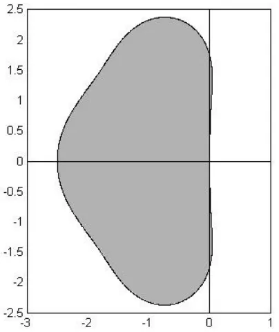
[image:4.595.319.521.72.312.2]

R z   z  (4.4) which is the stability polynomial of the method. The region of absolute stability is the region (in the complex plane) defined by |1R z( )| 1 (for a rigorous definition of stability, see [7]). Figure 1. shows the region of absolute stability for the scheme (2.11) obtained by using the MATLAB package [8].

Figure 1. Region of absolute stability for the numerical scheme (2.11).

5.

COMPUTATIONAL EXAMPLES

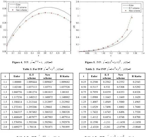
We illustrate the usefulness of our method by applying it to four examples. We compare the performance of the method with that of three other well-known methods, Euler's method, the Euler-Trapezoidal predictor-corrector method, with two corrections applied per step, and the Runge Kutta method. The performance of the proposed numerical scheme relative to the other methods is further illustrated in Tables 1-4, in which we tabulate numerical solutions of the four IVPs in Figures 2-5 using four different numerical methods. Notice that besides the numerical solutions of the three methods mentioned in Figures 2-5, the tabulated solutions include those obtained by the Runge Kutta method. MATLAB [8] was used to perform numerical computations and to generate the graphs in Figure 5.1

.

Figure 4. IVP: y e  yt, (0) 0y 

Figure 5. IVP: y( )ty3( / ) , (1) 1y t 2 y  Table 1: For IVP y t 2 y2, (1) 1y 

Table 2: For IVP y  1 t3 y2, (0) 0y 

t Euler E-T

scheme

New

scheme R Kutta t Euler

E-T scheme

New

scheme R Kutta 1.1 1.00000 1.009444 1.009667 1.009682 0.25 0.2500 0.2562 0.2552 0.2543

1.2 1.02100 1.037113 1.03751 1.037528 0.50 0.5117 0.532 0.5308 0.5292

1.3 1.060756 1.081274 1.081815 1.08183 0.75 0.7959 0.8359 0.8353 0.8328

1.4 1.117236 1.140212 1.140872 1.140882 1.00 1.0988 1.1643 1.1669 1.1620

1.5 1.188414 1.212144 1.212897 1.212902 1.25 1.4007 1.4949 1.5080 1.4965

1.6 1.272181 1.295206 1.29602 1.296024 1.50 1.6529 1.7498 1.8002 1.7680

1.7 1.366337 1.387482 1.388322 1.388328 1.75 1.7422 1.6745 1.8496 1.7520

1.8 1.468649 1.487077 1.487903 1.487914 2.00 1.4112 0.6874 1.0748 0.8700

1.9 1.576956 1.592186 1.592961 1.592978 2.25 0.1590 -1.211 -1.1450 -1.1850

2.0 1.689277 1.70118 1.701871 1.701895 2.50 -2.4320 -3.261 -2.8790 -3.0040

Table 3:For IVP y e  yt, (0) 0y 

Table 4: For IVP y( )ty3( / ) , (1) 1y t 2 y 

t Euler È-T

scheme

New

scheme R Kutta t Euler

È-T scheme

New

scheme R Kutta

0.25 0.250000 0.256230 0.255208 0.254342 1.03 1 1.002299 1.002272 1.00228

0.50 0.511719 0.532037 0.530759 0.529212 1.06 1.004504 1.009368 1.009294 1.009312

0.75 0.795933 0.835885 0.835346 0.832771 1.09 1.013778 1.021674 1.021521 1.021553

1.00 1.098841 1.164348 1.166901 1.161990 1.12 1.028306 1.039976 1.039701 1.039753

1.25 1.400704 1.494852 1.507986 1.496533 1.15 1.048847 1.065453 1.064982 1.065066

1.50 1.652916 1.749788 1.800248 1.767976 1.18 1.076536 1.099911 1.099119 1.099257

1.75 1.742199 1.674496 1.849619 1.751999 1.21 1.113064 1.146187 1.144846 1.145081

2.00 1.411170 0.687418 1.074768 0.869967 1.24 1.160967 1.208925 1.206581 1.207006

2.25 0.159020 -1.210912 -1.14489 -1.184548 1.27 1.224174 1.296276 1.291933 1.292771

[image:5.595.58.546.85.545.2]

6.

CONCLUSION

We have presented a numerical scheme that is efficient, stable and convergent. The implementation of the scheme is simple and the results obtained when the scheme is applied to various problems shows that the scheme compares favorably with other schemes. We have also given a comprehensive analysis of the convergence of the scheme and plotted the associated region of Absolute Stability

7.

ACKNOWLEDGMENTS

WS thanks the Directorate of Research Development of Walter Sisulu University for continued support. EAI would like to thank Walter Sisulu University for the Visiting Professorship opportunity and the authority of Ekiti State University, Ado-Ekiti, for granting him sabbatical leave to visit Walter Sisulu University. This research was conducted during his stay at Walter Sisulu University.

8.

REFERENCES

[1] Ackleh A.S., Kearfott R.B. and Allen E.J., 2010. Classical and Modern Numerical Analysis: Theory, Methods and Practice. Boca Raton: Chapman & Hall/CRC.

[2] Butcher J.C., 2003. Numerical Methods for Ordinary Differential Equations, John Wiley & Sons.

[3] Cheney W. and Kincaid D., 1999. Numerical Mathematics and Computing. New York: Brooks/Cole.

[4] Conte S.D. and de Boor C., 1980. Elementary Numerical Analysis: An Algorithmic Approach. New York: McGraw-Hill.

[5] Faires J.D., Burden R.L., 1993. Numerical Methods. Boston: PWS Publishing Company.

[6] Fatunla S.O., 1988. Numerical methods for initial value problems in ordinary differential equations. New York: Academic Press.

[7] Gear C.W., 1971. Numerical Initial-Value Problems in Ordinary Differential Equations. N.J.: Prentice-Hall, Englewood Cliffs.

[8] Gilat A., 2004, MATLAB: An Introduction with Applications. Michigan: John Wiley \& Sons.

[9] Henrici P., 1962. Discrete Variable Methods in Ordinary Differential Equations. New York: Wiley.

[10]Ibanez J, Hernandez V., Arias E. and Ruiz P.A., 2009. Solving initial value problems for ordinary differential equations by two approaches: BDF and piecewise-linearized methods, Comput. Phys. Commun. 180(5), 712--723.

[11]Ibijola E.A. and Kama P., 1999. On the convergence, consistency and stability of a one-step method for numerical integration of ordinary differential equation, Int. J. Comput. Math. 73(2), 261--277.

[12]Ibijola E.A. and Sunday J., 2010. A comparative study of standard and exact finite difference schemes for numerical solution of ordinary differential equations, Aust. J. Basic Appl. Sci. 4(4), 624--632.

[13]Lambert J.D., 1973. Computational Methods in Ordinary Differential Equations. New York: Wiley.

[14]Podisuk M., Chundang U. and Sanprasert W., 2007. Single step formulas and multi-step formulas of the integration method for solving the initial value problem of ordinary differential equations, Appl. Math. Comput. 190(2), 1438--1444.