Munich Personal RePEc Archive
Analytical Portfolio Value-at-Risk
Kaplanski, Guy
2005
Online at
https://mpra.ub.uni-muenchen.de/80216/
Analytical Portfolio Value-at-Risk
Guy Kaplanski*
Journal of Risk, Vol. 7, Issue 2, pp. 33-54, 2005
The author acknowledges the helpful comments of the editor Philippe Jorion, the anonymous referee and Oren Bar-Ner.
*
Analytical Portfolio Value-at-Risk
Abstract
The paper develops analytical tools used to calculate the VaR of a portfolio
composed of generally distributed assets. Accordingly, the VaR of a portfolio is
analytically constructed from the conditional returns of the individual assets. This
analytical VaR can then be used to construct optimal portfolios of generally
distributed assets for the case in which the target function and/or constraints are
expressed in terms of VaR. The proposed method is applicable in a wide range of
practical problems such as utility maximization under a VaR constraint. The article
demonstrates this method by developing a minimal VaR rule that identifies the
proportions that minimize the portfolio VaR. This rule is used to compare the
minimal VaR portfolio with the minimal standard deviation portfolio in the case of the
lognormal distribution. This example illustrates the importance of downside risk in
optimal asset allocation even under modest deviations from the normal distribution
such as in the case of the lognormal distribution.
Introduction
In recent years, Value-at-Risk (VaR) has become the standard tool used by
financial institutions to measure and manage risk.1 Currently, VaR is used primarily
for measuring market risk. However, there has been an increasing interest in using
the VaR concept as a tool for managing and regulating credit risk and as a
methodology for constraining and controlling the risk exposure of a portfolio.2 Most
studies that focus on VaR in the context of a portfolio either assume a simple normal
distribution or practically, use numerical calculations (see, for example, Campbell,
Huisman and Koedijk (2001) and Jorion (2001)). However, the widespread adoption
of VaR and other quantile measures in a portfolio framework calls for the
development of analytical methods to solve the portfolio optimization problem for
non-normal distributions and thereby to take full take advantage of these risk
measures. These methods are also required in order to improve and further develop
and explore VaR as a tool for risk measurement in a portfolio framework.
Assume, for example, the classical problem of optimal proportions between
the market shares portfolio and the market bonds portfolio such as in Campbell et al.
(2001). What is the portfolio VaR and how would the proportions of the two
portfolios influence this overall portfolio VaR? Usually, such a common problem is
solved either assuming the strong and restricting assumption of normal distribution or
by using a numerical approximation method. For example, Alexander & Baptista
(2002) assume either a normal distribution or a t-distribution when comparing VaR
and standard deviation in the context of mean-VaR analysis. Similarly, Sentana
(2001) analyzes the mean-variance frontier under a VaR constraint assuming
elliptically symmetric distributions, which can be fully defined by the first two
moments. However, this approach provides only an approximation in several
important cases where the distribution is not symmetrical or cannot be considered
elliptical. Differently, Emmer, Klüppelberg & Korn (2001), Cuoco, He & Issaenko
(2001), Yiu (2004) and others analyze the impact of a VaR constraint or some other
quantile constraint on asset allocation while using numerical techniques. This
approach might require large calculation resources and reckons on a possibly long
convergence process, especially when a range of compositions and strategies are
analyzed.
This article provides an alternative analytical method to solve such problems.
of generally distributed assets. Accordingly, the VaR of a portfolio is analytically
constructed from the conditional returns of the individual assets. This analytical VaR
can then be used to construct optimal portfolios of generally distributed assets for the
case in which the target function and/or constraints are expressed in terms of VaR.
The proposed method is appropriate for a wide range of applications. For example, it
can be used to analytically solve Basak & Shapiro’s (2001) problem of maximizing
utility under VaR constraint. Similarly, it can be used to expand the solution of Ahn,
Boudoukh, Richardson & Whitelaw’s (1999) problem in the realistic case of hedging
a portfolio with an option that is only partially correlated with the hedged portfolio.
The proposed method is demonstrated by developing a minimal VaR rule, which
identifies the proportions that minimize the portfolio VaR. A numeric example with
the lognormal distribution is then used to compare the minimal VaR with the minimal
standard deviation portfolios. This example highlights the importance of downside
risk in the context of portfolio asset allocation.
The paper is organized as follows: The next section develops the theoretical
relationship between the distribution of the individual assets and the VaR of the
portfolio. For simplicity, the presentation is confined to two assets (the generalization
to multiple assets can be found in Appendix B). Section II applies the findings from
Section I in order to develop a VaR minimization rule and to present a comprehensive
numerical example. Section III shows how the previous results can be used to solve
more complicated optimization problems such as Ahn, Boudoukh, Richardson and
Whitelaw’s (1999) problem of selecting a put option, which minimizes the portfolio
VaR. Section V concludes the paper.
I. Analytical Portfolio VaR
In this section, an analytical expression of the portfolio VaR is developed.
More specifically, the portfolio VaR is expressed in terms of the conditional
distributions of the individual assets and their proportions in the portfolio. The
information about these conditional distributions is equivalent to the information
about the assets cumulative distribution functions and their mutual correlations, which
is a prerequisite to solving any portfolio optimization problem. This is comparable to
the information about the means and the variance-covariance matrix required for the
classical Markowitz solution of the portfolio optimization problem. In order to
multiple asset portfolios together with an illustrative example are presented in
Appendix B).
Denote by X and Y the risky returns on any two assets with probability density functions, f(X)and g(Y), and cumulative distribution functions (cdf), F(X) and G(Y), respectively. In the proposed method, the correlation between X and Y is realized through the use of the conditional distribution. Therefore, without losing generality, let us select Y as the “unconditionally-distributed” asset and X as the “conditionally-distributed” asset. This selection does not indicate anything about the assets
themselves but rather implies that information about the correlation between X and Y
is given by the conditional distribution of X over Y. Namely, the roles of X and Y can be inverted. Intuitively, if the specific problem is involved with the market portfolio
or an index and a single asset, then selecting Y as the market portfolio corresponds to this model.
Let X(P) be the P-order quantile function of F(X). The quantile function is the inverse function of the cdf. Formally, X(P) is the maximum value of X for which there is a probability P of being below this value in the cdf of F(X) (namely, Pr(X X(P))=P). The quantile function is assumed to be monotonous. This
monotonicity is a direct result of the cdf monotonicity, which has been proved and
used by Rothschild and Stiglitz (1970) for the Second Stochastic Dominance analysis.
Let XY(P) be the conditional quantile of X on Y. Namely, XY(P) is the inverse function of the cdf of asset X conditional on Y, FY(X). By the same token, let Xy(P) be the conditional quantile of X on a specific realization y of Y.
VaR with a 1 Pˆ confidence interval, denoted as VaR(Pˆ ), can be defined as
the loss below some reference point t over a given period of time, where there is a
probability of Pˆ of incurring this loss or a larger one. In terms of the quantile
function, VaR(Pˆ ) can simply be written as
) ˆ ( )
ˆ
(P t X P
VaR . (1)
The reference point t can be a function of the cdf of X or a constant reference point,
such as the risk-free return or zero. For example, the official Basel (1996)
Amendment recommends calculating the VaR as the potential loss below the current
Proposition 1. The VaR of a Portfolio
Without losing generality, let be the proportion of X and 1- the proportion
of Y in a portfolio Z X (1 )Y. For any 0 < ,3 and for some selected
realization y of Y, the VaR of this portfolio is given by
y P
X t P
VaRZ(ˆ) y( *) (1 ) , (2)
where t is the loss reference point, Xy(P*) is the quantile of X conditional on a given
realization y, P* is solved by the expression
dY Y g y Y P
X F
Pˆ Y y( *) 1 ( ) ( ) , (3)
and the range of probabilities for which the specific realization y of Y provides a
solution of (2) is given by
dY Y g y Y X
F P dY Y g y Y X
FY y(0) 1 ( ) ( ) ˆ Y y(1) 1 ( ) ( ) . (4)
Proof
Denote the quantile of the portfolio Z = X + (1- )Y of orderPˆ as Z (Pˆ).
Denote the cdf of the portfolio Z conditional on asset Y as P** HY(Z ), where
0 P** 1. For a specific selected value y of Y, denote the cdf of the portfolio return at
point Z conditional on y as P* Hy(Z ), where 0 P* 1. According to Bayes’
Theorem (the “Total Probability Equation”)
dY Z H Y g Z
H
Pˆ ( ) ( ) Y( ) . (5)
Following Levy and Kroll’s (1978) quantile approach, the quantile of portfolio Z of
order P* conditional on realization y of Y can be written as
y P
X P
Zy( *) y( *) (1 ) , (6)
(for a proof of Levy and Kroll’s (1978) quantile approach see Appendix A).
According to the previous definitions of Pˆ and P*, we know that thePˆ -order quantile
of the unconditional return on the portfolio is equal to Z as is the conditional quantile
of order P* over y. Hence,
*) ( ) ˆ
(P Z P Z
From (6), (7) and the definition of P* we can conclude that for every value of Y either
there is an order 0<P**<1 such that the following holds
Y P
X y P
X
Z y( *) (1 ) Y( **) (1 ) , (8)
or for that specific y either
P** = 0, (8a)
or
P** = 1. (8b)
Note that (8a) and (8b) are required as the quantile function is defined over a finite
range. From (8), we get4
) ( *) ( *
* F X P 1 y Y
P Y y
. (9)
Combining (6) and (7) with the definition of VaR in (1) yields (2). Substituting
) ( *
* H Z
P Y from (9) into (5) yields (3). Finally, from the monotonuosity of the
quantile function it is sufficient to solve (5) for the two extremes P*=0 and P*=1 in
order to find the range of probabilities in (4) for which the specific realization y of Y
provides a solution to (2).
Discussion
Proposition 1 provides a method for calculating analytically the portfolio VaR
based on the conditional distributions of the individual assets. First, the order P* of
the quantile of X conditional on Y is implicitly solved by (3) and then it is substituted
into (2). The order P* is required as in general the P-order quantile of a portfolio is
not a linear combination of the individual quantiles.5
One might wonder how (2) and (3) yield the same VaRZ(Pˆ ) for any selected
realization y. The explanation lies in the fact that the integration in (3) is over all
values of Y and the arbitrary realization y of Y serves only as a reference and starting
point for this integration. Hence, the simultaneous effect of the selected y on both the
order P* in (3) and on the portfolio VaR in (2) completely offset each other such that
the total impact of the selection of y on the solution of the portfolio VaR is zero.
Nonetheless, the selected realization y might have an impact on the range of
probabilities for which there is a solution of Proposition 1, as is defined in (4).
Normally, this impact does not complicate the selection of y. This is because VaR is
order Pˆ ) such that (4) implies simply that the selected realization y should be
sufficiently small to contain the lower range of probabilities. In other words, except
for unique cases, when calculating VaR by Proposition 1 it is sufficient to choose a
sufficiently small realization y and solving (4) is not required practically. This issue is
further clarified in the following example.
An Illustrative Example
For illustration purposes, the following simplified example provides a
graphical exposition of Proposition 1. For simplicity of presentation, let the return on
Y be restricted to only two values, y1 and y2 with probabilities q and 1-q, respectively,
wherey1 < y2 (see Figure 1). In the following solution, y1 serves as the selected
realization. As has been previously mentioned, the intuition behind this selection is
that VaR is calculated usually over the lower left-hand side of the distribution and
therefore it is sufficient practically to simply choose a sufficiently low Y, in our case
y1, without actually solving (4). Later on, we also solve inequality (4) for a specific
example.
Assuming > 0, the conditional cdf of the portfolio for Y = y1 is given by
) (
1 Z
Hy . For any given order P, including the order Pˆ , Hy1(Z )divides the
horizontal difference between F(X) and y1 according to the proportions and (1- )
(see Figure 1 and Appendix A). Hence, according to (6), the conditional quantile is
given by
1
) 1 ( *) ( *)
( 1
1 P X P y
Zy y . (10)
Similarly,
2
) 1 ( *) * ( *)
*
( 2
2 P X P y
Zy y . (11)
Thus, from (10) and (11) we obtain
2
1 ( **) (1 )
) 1 ( *)
( 2
1 P y X P y
X
Z y y , (12)
or P** = 0 or P** = 1, depending on the distribution of X and the selected realization
y. According to Bayes’ Theorem in its discrete form
* * ) 1 ( *
ˆ qP q P
P . (13)
Finally, using (12) to extract P**and substituting it into (13) yields (3) in its discrete
form
Solving for P*, substituting it into (6) and deducting it from the reference point t,
yields (2) and produces the portfolio VaR.
For the purpose of demonstration, let us further assume that X is distributed
exponentially uncorrelated with Y, namely
, 0 , 0 ) exp( 1 ) ( ) ( other X X X F X
FY (15)
and 1 0 ) 1 log( 1 ) ( )
(P X P P P
XY . (16)
First, as Xy(0) 0 and Xy(1) , (4) in its discrete form yields
1 ) ( ) ( ˆ 0 ) ( ) ( 0 2 1 2 1 1 1 y y Y Y y y Y Y Y g y Y F P Y g y Y
F , for both
values of Y. Hence, in this specific case, both values of Y could be selected unrelated
to the required confidence interval.
Continuing with y1 as the arbitrarily selected realization, substituting (15) and
(16) into (14) yields two possible ranges. Assuming Xy1(P*) 1 (y2 y1) 0 or
equivalently P* 1 exp( 1 (y2 y1)), (14) yields
* ˆ Pˆ q(1 exp( 1 (y2 y1))) q
P
P . (17)
Assuming P* 1 exp( 1 (y2 y1)) yields
))) ( *) 1 exp(log( 1 )( 1 ( * ˆ 1 2 1 y y P q qP
P which yields
))) ( exp( 1 ( ˆ )) ( exp( ) 1 ( )) ( exp( 1 )( 1 ( ˆ
* 1 2 1
1 2 1 1 2 1 y y q P y y q q y y q P
P . (18)
Substituting the order P* from (17) and (18) into (2) yields the portfolio VaR
) 1 ( ) )) ( exp( ) 1 ( )) ( exp( 1 )( 1 ( ˆ -log(1 ))) ( exp( 1 ( ˆ 0 ) 1 ( ) ˆ -log(1 ) ˆ ( 1 1 2 1 1 2 1 1 2 1 1 y y y q q y y q P t y y q P y q P t P VaRZ 1 ˆ ))) ( exp( 1
( 1 y2 y1 P
[image:10.595.82.513.368.709.2]q . (19)
Figure 1 depicts the solution graphically for the case of assets X and Y in
proportions Z = 0.6X + 0.4Y (i.e. = 0.6). The return on asset X is exponentially
restricted to the two values, y1= 1 and y2= 2 with probabilities q = 0.3 and 1-q = 0.7.
Figure 1 reveals that the conditional cdf of the portfolio for Y = y1, H 1(Z )
y
, divides
the horizontal difference between F(X) and y1 according to the proportions = 0.6
and 1- = 0.4. Similarly, the conditional cdf of the portfolio for Y = y2, H 2(Z )
y
,
divides the horizontal difference between F(X) and y2 according to the same
proportions. It can also be seen in Figure 1 that Pˆ divides the vertical distance
between P* and P** according to the proportions 1 - q = 0.7 and q = 0.3. Similarly,
H(Z ) divides the vertical distance between the conditional cdfs Hy1(Z ) and
) (
2 Z
Hy according to the same proportions. Finally, using these characteristics, the
bold curve in Figure 1 graphically depicts the solution of (19).
The lower feasible range, (1- )y1 Z <(1- )y2 (i.e. 0.4 Z <0.8), can be
realized only when Y=y1 (as the minimal contribution of realization y2 to the total
portfolio value is the value y2 = 2 times its proportion in the portfolio of 0.4) . Hence,
the solution divides the vertical distance between the conditional cdf Hy1(Z ) and
P**=0 according to the proportions 1 - q and q. Finding this vertical weighted
average between Hy1(Z ) and P**=0 provides the solution in this range which is
given by the first range of (19). Correspondingly, the upper feasible range Z (1- )y2
(i.e. Z 0.8) can be realized under both realizations of Y. Hence, the solution divides
the vertical distance between the conditional cdfs Hy1(Z ) and Hy2(Z ) according
to the same proportions, 1 - q and q. Thus, finding the vertical weighted average
between Hy1(Z ) and Hy2(Z ) provides the solution in this range, which is given
by the second range of (19).
To sum up, equation (2) calculates the vertical weighted average between
) (
1 Z
Hy and Hy2(Z ) (or zero) at the order Pˆ and yields the Pˆ -order VaR.
Naturally, the solution of this simplified example of an asset, which is restricted to
only two values, is straightforward. However, the proposed method is general and the
same principles are applicable for any other, more complicated, case as is further
Generalization
Solving (3) for P*, which may be relatively complex in the case of numerous
assets (depending also on the conditional distribution), is quite simple in the case of
only few assets, as it requires the solution of only two equations. Furthermore, in this
case it has the advantage of yielding a unique analytical solution for any distribution
and with small calculation resources. Therefore, in the case of a small number of
assets, where the conditional distribution can easily be obtained, and when the
distribution cannot be considered normal, Proposition 1 provides a relatively simple
and straightforward solution. This case of small number of assets covers a wide range
of important problems. For example, Proposition 1 is best suited for solving
Campbell et al.’s (2001) problem of the optimal combination of shares and bonds
portfolios. In this important problem, in which at least one of the two assets cannot be
assumed to be normally distributed, it provides a unique solution, which requires
solving only two equations. This is in contrast to other numerical methods, which
might require a lengthy convergence process, and more seriously, might produce a
solution that is path-dependent of this convergence process. Other examples, which
are well suited for this method, are when optimization of VaR is required. For
example, Proposition 1 can be used to analytically find the minimal VaR portfolio as
is presented in the next section.
Another optimization example is analytically solving the agent’s optimization
problem presented in Basak & Shapiro (2001). In that problem, the agent maximizes
U(Z ) subject to
f y
Z P t X P y VaR
VaR (ˆ) ( *) (1 ) , (20)
which leads to the following constraint on the proportion of X in the portfolio
y P X
VaR y t
y
f f
*)
( , (21)
where VaRf is the required constraint floor, f is the bound on the proportion of X
which is induced by the constraint and the order P* is given in (3). Note that the
order P* in (21) is also a function of itself such that equality (21) may define both
upper and lower bounds on . Naturally, when the optimization problem involves
numerous assets the solution is more complex (see Appendix B). Another useful
example of only two assets, and therefore requires the solution of only two simple
Y, assuming the composition of Y is unchanged. Proposition 1 enables to fully study
that impact as a function of the composition of the overall portfolio. This ability is
further elaborated in the next section.
II. The Minimal VaR Portfolio in Case of Continuous Distributions
In this section Proposition 1 is used to analytically find the minimal VaR
portfolio in the case of two continuous and differentiable distributions. Then, an
illustrative numerical example is provided. This example demonstrates the advantage
of Proposition 1 over simulation techniques in calculating the VaR of a portfolio and
in VaR analysis when both assets are continuously distributed. This example is
further elaborated in order to compare between the minimal VaR and the minimal
standard deviation in the lognormal case. This comparison illustrates also the
importance of downside risk in optimal asset allocation even under modest deviations
from the normal case.
Let X and Y be the returns on two risky assets as in Proposition 1. If Xy(P) is
differentiable for a realization y of Y over the entire range 0 P 1, the proportion that
leads to the minimal VaR portfolio is solved by
*) ( *)
(
min y X P
d P
dXy y
, (22)
and the minimal VaR portfolio is given by substituting the proportion min in (2),
where the order P* is given by (3) as a function of Pˆ, y and the solution min. The
proof of (22) is straightforward. Differentiating the portfolio VaR, given by (2), with
respect to and equating it to zero in order to find the local minimum yields min,
which leads to the minimal VaR portfolio. Note that the differentiability of the
portfolio VaR and thus the existence of min is guaranteed as long as Xy(P) is
differentiable in the range 0 P 1.6
In the following, Proposition 1 and the implied minimal VaR rule in (22) are
used to analyze the VaR of a portfolio that is composed of lognormlly-distributed
assets. The lognormal distribution is appealing in many economic applications. This
is mainly because in contrast to the normal distribution the lognormal distribution is
able to capture the empirical phenomena of positive skewness and extra kurtosis as
well as the fact that risky returns are bounded from below. On the other hand, the
composed of lognormally distributed assets is not lognormally distributed and does
not have an analytical expression. Thus, the VaR of the combined portfolio cannot be
found straightforwardly and an approximation or a numerical technique is usually
required. Proposition 1 provides a simple solution for this shortcoming as is shown
below. In Appendix B this example is expanded to a more realistic case of a
three-asset portfolio.
Let X and Y be multivariate lognormally distributed with expected returns and
standard deviations of the logs of X, Y, X and Y, respectively, and with correlation
coefficients of the logs of . Namely, log(X) and log(Y) are multivariate normally
distributed with the above parameters. Hence,
) 2 ) ( exp( 2 1 ) ( 2 2 2 Y Y Y B Y Y
g , (23)
for Y > 0 and zero for other,
) ) 1 ( 2 ) ) ( ) ( ( exp( ) 1 ( 2 1 ) ( 2 2 2 2 2 X y x X Y Y B X B X X
f , (24)
and ) ) 1 ( ) ( ) ( ( ) ( 2 2 X Y X N Y Y B X B F X
F , (25)
for X > 0 and zero for other, and
) ) 1 ( ) ( ) ( exp( )
( 2 X2
Y X X Y P N Y B P
X , (26)
for 0 P 1, where FN and N(P) are the cdf and the P-order quantile of the normal
standard distribution and B(X) log(X) X . From (2), the portfolio VaR is given by y P N y B t P VaR X Y X X
Z(ˆ) exp( ( ) ( *) (1 ) ) (1 )
2 2
, (27)
where, from (3), the order P* is solved implicitly by
dY Y B
Y Y
B
Y Y
X Y X X
) 2
) ( exp( 2
1 ) )
1 (
) (
2 2
2 2
2 . (28)
Thus, finding the VaR of the portfolio requires solving implicitly the order P* from
(28) and substituting it in (27). This is a relatively simple task, which does not
involve numerous iterations as might be in other numerical methods.
Continuing with this example, the same technique can be used to find the
minimal VaR portfolio. By chain differentiation we can rewrite (22) as7
*) (
) ( )
(
min
P X y
dY Y A YdY Y A y
y , (29)
where A(Y) g(Y)fY Xy(P*) 1 (Y y) , g(Y), fY(X) and Xy(P*) are given by
(23), (24) and (26) (only with y instead of Y), the order P* is solved by (3) and y is
any arbitrarily selected realization of Y (as the ranges of X and Y are identical).
Figure 2 presents a numerical example of the above results. Panel A plots the
mean-VaR frontier of two independent lognormally-distributed assets with the
following parameters:X ~ (2.4,0.136) andY ~ (2.3,0.15), where for simplicity,
t=0 and the confidence interval is either 99 percent or 95 percent. The VaR at each
point on the curves is calculated by solving implicitly for P* from (28) and then
substituting it in (27). Thus, each point on the curves requires solving only two
equations together with the trivial equation of the portfolio expected return, EZ = EX
+(1- )EY. This is comparable with a simulation method, which might require several
hundred samples for each point in order to guarantee plausible accuracy. This
advantage is even more apparent when calculating the minimal VaR portfolio.
The horizontal curve in Panel A plots the minimal VaR portfolio as a function
of the required confidence interval using equation (29). Once again, each point on the
curve requires to solve only the two equations, (28) and (29). In contrast, a simulation
method might require an iterative convergence process in which each iteration, which
takes the VaR closer to the minimal VaR, might be involved also with numerous
samples.
Panel B of Figure 2 plots the mean-VaR frontier for a 99 percent confidence
previous example, these curves demonstrate the relative simplicity of calculating the
portfolio VaR at each point using equations (27) and (28). In addition, this example
shows the impact of correlation on the portfolio VaR, which, as expected, is
analogous to the impact of correlation on the portfolio standard deviation. However,
in spite of this similarity there are also important differences as are presented below.
Figure 3 juxtaposes the proportion of X, which leads to the minimal VaR
portfolio, min, calculated by (29) with the proportion of X, which leads to the minimal
standard deviation portfolio8 in the lognormal case. This comparison shows that even
under the modest deviation from the normal distribution of assuming a lognormal
distribution there are critical differences between VaR and standard deviation and
between the implied optimal asset allocation according to these risk measures. It is
plausible to assume that the differences would be even larger in the case of empirical
distributions. Each point on the curves in Figure 3 represents the proportion of X in
the minimal VaR portfolio ( min) and in the minimal standard deviation portfolio for
portfolios constructed from two independent lognormally-distributed assets, X and Y.
Namely, at each point the assets’ returns have different parameters. Panel A plots
min as a function of the ratio between the expected returns of X and Y with standard
deviations held constant.9 The calculations are done for three different ratios of the
standard deviations of X and Y, where the standard deviation of X is equal to 1.5 and
the standard deviation of Y is 0.5, 1.5 and 2.5. Panel B plots min as a function of the
ratio of the standard deviations of X and Y while the expected returns of X and Y are
held constant. The calculations are done for three different ratios of the expected
returns of X and Y, where the expected return of X is equal to 10 and the expected
return of Y is 9,10 and 11.
The results emphasize the differences between VaR and standard deviation
risk measures and the impact of downside risk on assets allocation. The curves on
Panel A show that for a given ratio of standard deviations, a higher expected return of
X relative to that of Y does not affect min which leads to the minimal standard
deviation. In contrast, a higher expected return of X relative to that of Y leads to a
higher min which leads to the minimal VaR. For example, a difference of 20 percent
between the expected returns of X and Y (namely, EX /EY 1.2) leads to a proportion of X that is greater than 0.95 in the minimal VaR portfolio. Furthermore, this result is
both values of min behave similarly when the standard deviation is changed, there is a
significant quantitative difference between the results, which depends on the relations
between the expected returns.
In summary, Figure 3 reveals that the relationship between the minimal VaR
and the minimal standard deviation in the case of the lognormal distribution is
significantly different from the relationship in the case of the normal distribution.
Alexander & Baptista (2002) show that in the case of a multivariate normal
distribution, if the minimum VaR portfolio exists, then it lies above the minimum
variance portfolio on the mean-standard deviation frontier. According to Figure 3 this
does not hold in the case of the lognormal distribution.
The results of Figure 3 illustrate the basic conceptual difference between
standard deviation and VaR. Theoreticians, as well as practitioners, conceptually
view risk as the chance of obtaining poor results relative to a given reference point
(such as expected return, the risk-free interest rate or zero). However, standard
deviation measures the dispersion around the mean and reflects correctly the
downward risk of two alternative prospects only when their means are equal or when
distributions are symmetrical. Unlike the standard deviation, VaR measures
downward risk in terms of potential loss under specifically defined probability. Thus,
VaR considers the mean and dispersion as well as all higher moments. Therefore,
substantial differences should be expected between the two measures and the implied
assets allocation even when it is the higher moments that are being varied.
III. Analytical VaR and Ahn, Boudoukh, Richardson and Whitelaw (1999) Analysis
Ahn et al. were the first to develop an analytical VaR optimization solution.
They confined themselves to the case of hedging a lognormally-distributed asset with
a put option on the managed portfolios. In Ahn et al.’s analysis, X is a put option on
an underlying asset Y, which is assumed to terminate in-the-money. Ahn et al. then
compute the optimal strike price that minimizes VaR. Below we show how their
problem can be extracted from our proposed method. Although in Ahn et al.’s
specific case it is simpler to formulate the problem straightforwardly, the proposed
under more complex but yet realistic conditions whereby the optimized portfolio
includes various types of assets including derivative assets that are only partially
correlated with the hedged portfolio.
Ahn et al. assume a fixed hedging expense of C=hq, where h is the number of
options and q is the price of each option. They also assume that this expense is
financed by a loan with a continuous interest rate r such that the amount to be repaid
in the future is rt
qe per option. Thus, the fixed hedging expense C determines the
portfolio assets allocation ( X h, r h , Y 1) and using equation (B1) we get the general problem of minimal VaR of a three asset portfolio
] *)
( [
min t hX y,r P hqert y , (30)
where P* is solved from (B2). The formulation of the problem in (30) is general as it
is correct for any distribution and any correlations between the three assets. In Ahn et
al. specific case, the quantile of the put option conditional on the underlying asset
(which is of course also conditional on the risk-free interest rate as required by (30)) is
given by Xy(P*) K y, where K is the option strike price and y is necessarily the
Pˆ -order quantile of Y (since in the case of a put option with full correlation
P
P* ˆand there is only one value of X for each realization y of Y). Substituting
*) (P
Xy in (30) yields
] ) 1 ( min[
] )
(
min[ y
q C Ce K q C r y
hqe y K h
t rt rt
max[ ] max[ ] q
y K q
y K
C . (31)
Finally, by assuming that the underlying asset Y is lognormally-distributed, such that y
is equal to the Y's Pˆ -order lognormal quantile, we arrive at Ahn et al.'s original
minimization problem (see equation (16) in Ahn et al.).
Clearly, it is simpler in case of a full correlation to formulate the problem
straightforwardly, as Ahn et al. do. However, their assumption that there is a traded
put option on the underlying asset scarcely exists. In general, traded options are not
written on institutional portfolios but only on specific assets and indexes. Equation
(30), which is based on the proposed model, makes it possible to solve the optimal
strategic hedging problem under more realistic conditions whereby the options and
can also deal with more complicated problems in which the portfolio includes various
types of derivatives and financing is not restricted only to debt. The following
example demonstrates these advantages.
Let us assume that in a hedging problem similar to Ahn et al., the agent faces
more realistic market terms. For the purpose of demonstration, suppose that the agent
faces two types of put options, X1 and X2 written on two market indices, which are
uncorrelated with each other and only partially correlated with the agent portfolio.
Assume also that the agent searches for the combination of options that minimize the
total VaR of her portfolio. Hence, the fixed hedging expense, C, can be used to buy
two types of options. Namely, C = h1q1+ h2q2, where h1 and h2 are the number of
options of the first type and the second type and q1 and q2 are the prices of each
option, respectively. Assume, as in Ahn et al., that the hedging expense is financed
by a loan with a continuous interest rate r such that the amount to be repaid in the
future is qiert per option. Thus, the fixed hedging expense C determines the portfolio
assets allocation to be 1, 2 , ( 1 2)and 1 2
1 X r Y
X h h h h . Recall that the
conditional quantile function of the first type of option is uncorrelated with the second
type option and with r (i.e.X1x2y,r(P*) X1y(P*)) and h
2=(C-h1q1)/ q2, equation (B1)
formulates the optimization problem to be
] *)
( [
min 2
2 1 1 1
1 1
x q
q h C y Ce P
X h
t y rt
h , (32)
where, from (B2), P* is solved by
2 2
2 2
2 1
1
1 ( ( *) ( ) ( )) ( ) ( )
ˆ
1 2
1 1
1 Y y X x g Y f X dYdX
P X F
P Y y h Cqhhq , (33)
and g(Y) and f(X2) are the probability density functions of Y and X2. Finally,
substituting the conditional quantile function and cdf fully formulate the optimization
problem, which can then be easily solved.
IV. Concluding remarks
This paper develops analytical tools for extracting the VaR of a portfolio from
the general distributions of its underlying assets. This analytical VaR can then be
which the target function and/or constraints are expressed in terms of VaR. The basic
information required for this problem is the conditional distributions of the risky
assets. This is analogous to the information about the means and the
variance-covariance matrix required for the classical Markowitz optimal portfolio problem.
This proposed method can be used to solve any optimization problem, which involves
portfolio VaR and is applicable to any distribution, not only the problematic normal
distribution.
The proposed method is used to develop a minimal VaR rule, which identifies
the minimal attainable VaR. The paper presents a detailed illustrative example of a
portfolio composed of two dependent lognormally-distributed assets. This example
emphasizes the advantage of the proposed method since it enables overcoming the
main drawback of the lognormal distribution, i.e. that the distribution of a portfolio
composed of lognormally distributed assets cannot be expressed analytically.
Accordingly, the proposed method makes it possible to calculate straightforwardly the
portfolio VaR by solving two simple equations. In our particular example, the
solution is used to compare between the minimal VaR portfolio and the minimal
standard deviation portfolio in the case of the lognormal distribution. This
comparison reveals that the optimal proportions that minimize the VaR depend on all
moments of the distribution. This intuitive outcome highlights the importance of
using the correct measure of risk and the deficiencies of the standard deviation in this
regard. Thus, this example illustrates the simplicity and the efficiency of the proposed
method especially in the case of a portfolio that is composed of only a small number
of assets.
This case covers many practical problems in finance. For example, this
method is best suited to analyze the Campbell, Huisman and Koedijk (2001) problem
of the optimal combination of shares and bonds portfolios. Similarly, this method is
well suited to find the minimal VaR portfolio and to analyze the impact of adding an
asset to an existing portfolio on the overall portfolio VaR. Finally, the paper uses the
proposed method to formulate the problem of Ahn, Boudoukh, Richardson and
Whitelaw (1999) of minimizing the portfolio VaR with a put option. This additional
example demonstrates the ability of this method to analytically formulate
complicated, realistic VaR optimization problems such as when the hedging
Appendix A: The Quantile Function of a Portfolio Composed of Risky and Risk-Free Assets
The following proof of the quantile function of a portfolio composed of risky
and risk-free assets is taken from Levy and Kroll (1978). Let X be an asset with a
random return with a cdf F(X) and a quantile function X(P). Denote the mixture of X
with the risk-free asset by Z . Thus, Z (1 )r X where 0 < and r is the
risk-free interest rate. Recall that by definition
F(X(P)) Pr(X X(P)) P. (A1)
Thus, since and r are constants (A1) implies that for any 0 < the following holds
Pr((1 )r X (1 )r X(P)) P. (A2)
Substituting the definition of Z from above into (A2) yields
Pr(Z (1 )r X(P)) P. (A3)
However, since by definition Pr(Z Z (P)) P, where Z (P) is the quantile
function of the portfolio, then by necessity
) ( )
1 ( )
(P r X P
Appendix B: Analytical VaR of Multiple Asset Portfolios
In the following the model is extended to the case of a multiple asset portfolio.
The proofs in this case are identical to those of the two-assets case and will not be
repeated.
Let Xi (i=1…n) be the returns on n risky assets with probability density
functions fi(X)and cumulative distribution functions (cdf) Fi(X). Let
n i iXi
Z
1
be the random return on a portfolio composed of these n assets. Let Xxi(P)
j be the
quantile of the return on asset Xj conditional on the vector of realizations xi of Xi
(i=1…n, i j). The information about this conditional quantile is tantamount to the
information about the assets’ cdfs and the relationship between them and obtaining it
is a prerequisite to solving any portfolio optimization problem.
Proposition B1. For every 0 i 0< j (i=1,…n, i j) and some selected vector of
realizations xi of Xi which guarantees that 0 P* 1, the VaR of the portfolio Z is
given by n j i i i i x j j
Z P t X P x
VaR i 1 *) ( ) ˆ
( , (B1)
where the order P* is solved from the following equation
i i i n j i i n j i i i i x j X dX X f x X P X F P j i i
i( ( *) ( )) ( )
... ˆ
1 1
. (B2)
Note that the integration in (B2) is over n-1 variables. The range of probabilities for
which the vector of realizations xi of Xi provides a solution of (B2) is given by
P dX X f x X X
F i i i
n j i i n j i i i i x j X j i i
i( (0) ( )) ( ) ˆ
... 1 1 . i i i n j i i n j i i i i x j X dX X f x X X F j i i
i( (1) ( )) ( )
...
1 1
. (B3)
Contentiously with the analogy to the two-asset case, assuming that Xxi(P)
j is
differentiable for any order P in the range [0,1] and for any vector of realizations xi of
Xi (i=1…n, i j), which is required in order to guarantee that the portfolio distribution
is well behaved, the proportions of the minimal VaR portfolio, mini (i=1,…n), are
*) ( *
( min
j x X P
d P dX i i x j n j x j
, (B4)
together with the following n-2 equations
j i ...n-i x x d P dX i n i x j i , 1 1 , *) ( min
i , (B5)
and the trivial equation
1 1 1 n i i
n , (B6)
where P* is simultaneously solved from (B2) as a function of Pˆ , imin and xi. Finally,
the minimal VaR is obtained by substituting imin (i=1,…n) into (B1).
An Illustrative Example
Let X be the return on a bank commercial activity. Let Y and W be the return on the
bank domestic and foreign financial investment portfolios, respectively. Let X and Y
be multivariate lognormally distributed with expected returns and standard deviations
of the logs of X, Y, X and Y, respectively, and with correlation coefficients of the
logs of . Let W be lognormally distributed with expected return and standard
deviation of the log of W and W uncorrelated, as being a foreign market, with X and
Y. Denote the bank total portfolio as Z 1X 2Y 3W, 0 2,3 0< 1.
According to preposition (B1), and using the identities of g(Y) given by (23), FY,W(X)
= FY(X) given by (24), and Xy,w(P) = Xy(P) given by (26), the bank overall VaR is
given by w x P N y B t P VaR X Y X X
Z 2 3
2 2
1exp( ( ) ( *) (1 ) )
) ˆ
( , (B7)
where the order P* is solved from the following equation
dYdW W h Y g w W y Y P X F
P YW yw
) ( ) ( )) ( ) ( *) ( ( ˆ 1 3 1 2 , ,
= (B8)
0 0 2 2
and where 3 1 2 1 and B(W) log(W) W.
Thus, as in the two-asset case, finding the VaR of the overall portfolio requires
implicitly solving the order P* from (B8) and substituting it in (B7). This relatively
simple task can be easily used to map the impact of the proportion of the foreign
portfolio on the bank overall VaR. For example, assuming the value of the bank
financial investment portfolio to be 10% (i.e. 3 2 0.1) solving (B7) and (B8)
for a vector of values in the range 2 0,0.01,0.02...0.1 will map the full scope of the
impact of international diversification on the bank VaR. This is achieved by solving
REFERENCES
Ahn, D.H., Boudoukh, J., Richardson, M., and R.F., Whitelaw, "Optimal Risk Management Using Options", J. of Finance, 54(1), February 1999, 359-375.
Alexander, J.G., and A.M., Baptista, "Economic Implications of Using a Mean-VaR Model for
Portfolio Selection: A Comparison with Mean-Variance Analysis", Journal of Economic Dynamics and Control, 2002, 1159-1193.
Artzner, P., Delbaen, F., Eber, J.M., and D., Heath, "Coherent Measures of Risk", Mathematical Finance, 9, 1999, 203-228.
Basak, S., and A., Shapiro, "Value-at-Risk Based Risk Management: Optimal Policies and Asset Prices", Review of Financial Studies, 14(2), 2001, 371-405.
Basel Committee on Bankig Supervision, Amendment to the Capital Accord to Incorporate Market Risks, January 1996.
Campbell, R., Huisman, R., and K., Koedijk, "Optimal Portfolio Selection in a Value-at-Risk Framework", J. of Banking and Finance, 25, 2001, 1789-1804.
Crouhy, M., Galai, D., and R., Mark, Risk Management, (Eds.), McGraw-Hill, 2001.
Cuoco, D., He, H., and S., Issaenko, "Optimal Dynamic Trading Strategies with Risk Limits",
University of Pennsylvania working paper, 2001.
Duffie, D., and J., Pan, "An Overview of Value at Risk", J. of Derivatives, 4, Spring 1997, 7-49.
Duffie, D., and J., Pan, "Analytical Value-at-Risk with Jumps and Credit Risk", Finance and Stochastic, 5, 2000, 155-180.
Emmer, S., Klüppelberg, C., and R., Korn, "Optimal Portfolios with Bounded Downside Risks",
Mathematical Finance, 2001, 365-384.
Harvey, C.R., and A., Siddique, "Conditional Skewness in Asset Pricing Tests", J. of Finance, 55, June 2000, 1263-1295.
Jorion, P., Value at Risk: The New Benchmark for Managing Financial Risk, McGraw-Hill, December 2000.
Jorion, P., "Portfolio Optimization with Constraint on Tracking Error", Working paper, University of California at Irvine”, 2001.
Kaplanski, G., and Y., Kroll, "VaR Risk Measures versus Traditional Risk Measures: An Analysis and a Survey ", Journal of Risk, 4(3), 2002, 1-27.
Levy, H., and Y., Kroll, "Ordering Uncertain Options with Borrowing and Lending", J. of Finance, 33(2), May 1978, 552-573.
Rothschild, M., and J.E., Stiglitz, "Increasing Risk. I: A Definition", J. of Economic Theory, 2, 1970, 225-243.
Sentana, E., "Mean Variance Portfolio Allocation with a Value at Risk Constraint", C.E.P.R.,
Discussion Papers, 2997, 2001.
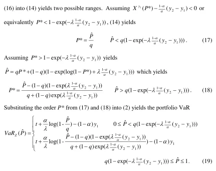
Figure 1. A graphical expositionof Proposition 1
The figure plots the construction of a VaR value for a portfolio composed of assets X and Y in proportions Z = 0.6X + 0.4Y. The return on asset X is exponentially distributed with parameter = 1 uncorrelated with the return on asset Y which is restricted to two values, y1=1and y2=2 with
probabilities q = 0.3 and 1-q = 0.7. The conditional cdf of the portfolio for Y=y1, H 1(Z ) y
, divides
the horizontal difference between F(X) and y1 according to the proportions = 0.6 and 1- = 0.4.
Similarly, the conditional cdf of the portfolio for Y=y2, H 2(Z ) y
, divides the horizontal difference
between F(X) and y2 according to the same proportions. It canbe seen in Figure 1 that Pˆ divides the
vertical distance between P* and P** according to the proportions 1 - q = 0.7 and q = 0.3. Similarly,
H(Z ) divides the vertical distance between the conditional cdfs Hy1(Z ) and Hy2(Z )according to
the same proportions.
Probability
P*
1-q
Pˆ
P** q
1-
1-
F(X) Hy1(Z ) H(Z )
Hy2(Z ) G(Y)
y1= Z y2=
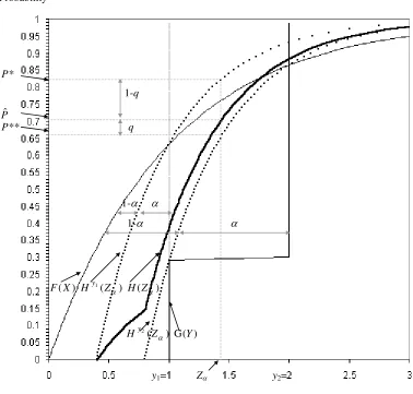
Figure 2. Portfolio VaR of two lognormally-distributed assets
The figure plots the mean-VaR frontier of a portfolio composed of two lognormally-distributed assets with the following parameters: X ~ (2.4,0.136) and Y ~ (2.3,0.15) and assuming also t=0. Panel A plots the mean-VaR frontier for 95 and 99 percent confidence intervals assuming independent distributions (namely, =0). The horizontal curve plots the minimal VaR as a function of the confidence interval. Panel B plots the mean-VaR frontier of a portfolio composed of the same assets assuming a correlation coefficient of =–0.5, 0, 0.25 and 0.9. Each point on the curves requires to solve only the two equations (27) and (28).
Pˆ 5% Pˆ 1% X X
Minimal VaR 1% Pˆ 8%
Y Y
X
= -0.5 = 0 = 0.25 = 0.9
Y
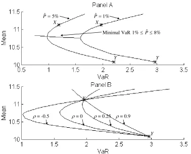
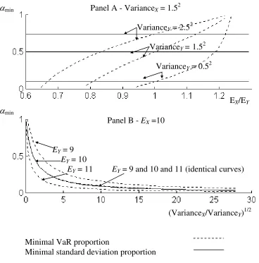
Figure 3. The minimal VaR portfolio versus the minimal standard deviation portfolio
Panel A plots the proportion of asset X in the minimal VaR portfolio versus the proportion of asset X in the minimal standard deviation portfolio, for different independent assets X and Y, as a function of the ratio between the expected returns of assets X and Y. Panel B plots the same as a function of the ratio between the standard deviations of X and Y. The curves illustrate the importance of downside risk in asset allocation and the critical distinction induced by VaR and standard deviation on the portfolio asset allocation even under modests deviation from the normal distribution.
min Panel A - VarianceX = 1.52
VarianceY = 2.52
VarianceY = 1.52
VarianceY = 0.52
EX/EY
min
Panel B - EX =10
EY = 9
EY = 10
EY = 11 EY = 9 and 10 and 11 (identical curves)
(VarianceX/VarianceY)1/2
Minimal VaR proportion
1
An introduction and overview of VaR can be found in Duffie & Pan (1997) and in the excellent books by Jorion (2000) and Crouhy, Galai & Mark (2001).
2
For more on credit risk issues see, for example, Duffie & Pan (2000). For more on the methodology used to constrain and control risk exposure see, for example, Basak & Shapiro (2001) and Jorion (2001).
3
Assuming 0< eliminates short sales of asset X. This assumption can easily be dropped by replacing
P* in (2) and (3) for < 0 by the expression 1-P*. Then, if < 0 the VaR of the portfolio is given by
y P
X t P
VaRZ(ˆ) y(1 *) (1 ) , and P* is solved by the expression
dY Y g y Y P X F
Pˆ Y y(1 *) 1 ( ) ( ) .
4
In (9) we do not need to specify separately the cases of (8a) and (8b) as, unlike the quantile function, the cdf function is defined over the entire range.
5
The order P is stable in a linear combination only when the portfolio is composed of a risky asset and a risk-free asset or in the trivial case of fully correlated assets. Indeed, if Y is the risk-free asset r, then Proposition 1 converges to Levy & Kroll's (1978) solution of a portfolio of a risky asset and a risk-free asset. Substituting Y = r in (3) yields
* * ) ( ) ( *) ( ˆ 1 P dr P dr r g r r P X F
P r r and substituting Pˆ P* in (2)
yields VaRZ(Pˆ) t X(Pˆ) (1 )r which corresponds to the results of Kroll & Levy (see
equation (3) there and in Appendix A).
6
In (22) it is assumed that VaR is an increasing monotonic function around min. This assumption is
correct by definition in the immediate neighborhood of min as long as min exists since we define min
as the proportion that leads to the local minimal VaR. Furthermore, min always exists in our case since
the assumption that the conditional quantile Xy(P*) is differentiable guarantees the monotonicity of VaR. In fact, VaR monotonicity for contiguous and differentiable quantiles derives from the
monotonicity of the portfolio cdf, which, as has been previously said, is proved and used by Rothschild and Stiglitz (1970) for the case of Second Stochastic Dominance analysis. Corresponding with Artzner et al. (1999), this property does not exist for VaR in the case of discrete distributions. Nevertheless, it should be kept in mind that discrete distributions are usually empirical approximations of actual continuous distributions.
7
The only mathematical manipulation is the use of chain differentiation in order to solve (22).
Accordingly, equation (22) is rewritten as:
* ˆ ˆ * *) ( *)) ( ( min dP P d d P d dP P dX P X y y y and
from (3) we obtain the following identities:
dY dP P dX y Y P X f Y g dP P
d Y y y
* *) ( ) ( *) ( ) ( * ˆ 1 and dY y Y y Y P X f Y g d P
d Y y
2 1 ) ( *) ( ) ( ˆ . 8
The proportion which leads to the minimal standard deviation portfolio is given by:
Y X Y X Y X Y 2 2 2 2 min . 9