26
An Efficient Modified Shuffled Frog Leaping Optimization
Algorithm
Mohammad Pourmahmood
Aghababa
Department of Electrical
Engineering, Ahar Branch, Islamic
Azad University, Ahar, Iran
Mohammd Esmaeel Akbari
Department of Electrical
Engineering, Ahar Branch, Islamic
Azad University, Ahar, Iran
Amin Mohammadpour
Shotorbani
Department of Electrical Engineering,
Azerbaijan University, E. Azerbaijan,
Iran
ABSTRACT
In this paper, a modified shuffled frog leaping (MSFL) algorithm is proposed to overcome drawbacks of standard shuffled frog leaping (SFL) method. The MSFL approach is based on two major modifications on the conventional SFL method: (1) an adaptive accelerated position changing of frogs and (2) sweeping between randomly selected frogs (called superseding frogs). The first modification causes a fast convergence rate and consequently achieving a rapid adaptive algorithm, while the second one causes a better diversification and consequently escaping from local optimum traps. The MSFL algorithm performance is validated using benchmark functions. Simulation results indicate the superiority of MSFL to that of the original SFL in terms of optimal precision and fast convergence rate.
Keywords
Shuffled frog leaping algorithm, Optimization approach, Convergence rate, Escaping local optimum.
1.
INTRODUCTION
The objective of optimization is to seek values for a set of parameters that maximize or minimize objective functions subject to certain constraints. In recent years, many optimization algorithms are introduced. Some of these algorithms are traditional optimization algorithms. Traditional optimization algorithms use exact methods to find the best solution. The idea is that if a problem can be solved, then the algorithm should find the global best solution. As the search space increases the objective value of these algorithms increases. Therefore, when the search space complexity increases the exact algorithms can be slow to find the global optimum. Linear and nonlinear programming, brute force or exhaustive search and divide and conquer methods are some of the exact optimization methods.
Calculus provides the tools and elegance for finding the optimum value of many objective functions. It quickly finds a single optimum but requires a search scheme to find the global optimum. Continuous functions with analytical derivatives are necessary (unless derivatives are taken numerically, which results in even more function evaluations plus a loss of accuracy). If there are too many variables, then it is difficult to find all the extrema. The gradient of the objective function serves as the compass heading solution to the steepest downhill path. It works well when the optimum is nearby, but cannot deal with cliffs or boundaries, where the gradient cannot be calculated.
Other optimization algorithms are stochastic algorithms, consisted of intelligent, heuristic and random methods. Stochastic algorithms have several advantages compared to other algorithms as follows:
1) Stochastic algorithms are generally easy to implement.
2) They can be used efficiently in a multiprocessor environment.
3) They do not require the problem definition function to be continuous.
4) They generally can find optimal or near-optimal solutions.
Nowadays, artificial intelligence techniques have found many successful applications in science and engineering (for example see Refs. [1-10] for intelligent PID controller design). Evolutionary algorithms (EAs) are stochastic optimization methods that mimic the metaphor of natural biological evolution and/or the social behavior of species. Shuffled Frog Leaping (SFL) [11, 12] is one of the new EAs that has been proposed by Eusuff and Lansey for determining optimal discrete pipe sizes for new pipe networks and for network expansions [11]. It is based on evolution of memes carried by the interactive individuals and a global exchange of information among themselves. The SFL works based on memetic evolution (transformation of frogs) and information exchange in the population. Frogs which are the hosts of memes (consisting memotype like gene in chromosome in GA) search the particle with the highest amount of food in a swamp by improving their memes. This characteristic can be used in an intelligent manner in control systems.
This paper proposes the MSFL technique as a new optimization algorithm. The proposed method is applied for determining the optimal values for some benchmark functions. The advantages of this methodology are that it is a simple method with less computation burden, high-quality solution and stable convergence specifications.
The rest of this paper is organized as follows. In section 2, an overview of SFL algorithm is given. In Section 3, the modified version of SFL is introduced. Using some benchmark functions, the efficiency of the proposed MSFL is illustrated in Section 4. Finally, the paper ends with some conclusions in section 5.
2.
SFL ALGORITHM
27 algorithm uses memetic evolution in the form of influencing of
ideas from one individual to another in a local search. Conceptually, the local search is similar to particle swarm optimization. A shuffling strategy allows the exchange of information among local searchers, leading them toward a global optimum [11].
In SFL, the population consists of a set of frogs (solutions) partitioned into subsets, referred to as memeplexes. Different memeplexes are considered as different cultures of frogs, each performing a local search. Within each memeplex, the individual frogs hold ideas, that can be influenced by the ideas of other frogs, and evolve through a process of memetic evolution. After a defined number of memetic evolution steps, ideas are passed among memeplexes in a shuffling process [12]. The local search and the shuffling processes continue until some predefined convergence criteria are satisfied [11].
In general, a SFL works as follows. First, an initial population of P frogs is created randomly. Afterwards, the frogs are sorted in a descending order according to their fitness. Then, the entire population is divided into m memeplexes, each containing n frogs. In this process, the first frog goes to the first memeplex, the second frog goes to the second memeplex, frog m goes to the mth memeplex, and frog m+1 goes back to the first memeplex and so on. Within each memeplex, the frogs with the best and the worst fitnesses are identified as Xb and Xw, respectively. Also, the frog with the global best fitness is identified as Xg. Then, a process is applied to improve only the frog with the worst fitness (not all frogs) in each cycle.
Accordingly, the position of the frog with the worst fitness is adjusted as follows [11]:
Chang frog position:
Di=rand × (Xb - Xg ) (1)
New position:
Xi+1 =Xi +Di where -Dmax ≤Di ≤ Dmax, (2)
where rand is a random number between 0 and 1, and Dmax is the
maximum allowed change in a frog’s position. If this process produces a better solution, it is replaced for the worst frog. Otherwise, the calculations in equations (1) and (2) are repeated but with respect to the global best frog (i.e. Xb is replaced by Xg).
If no improvement is possible, then a new solution is randomly generated to replace the worst frog. Hence, the calculations continue for a specific number of iterations [11]. Accordingly, the main parameters of SFL are: number of frogs P; number of memeplexes; number of generation for each memeplex before shuffling; number of shuffling iterations; and maximum step size.
3.
MODIFIED SHUFFLED FROG
LEAPING ALGORITHM
The main drawback of SFL algorithm is slow convergence, closely related to the lack of adaptive acceleration terms in the position updating formula. In equation (1), rand determines the movement step sizes of frogs through the Xb and Xw positions. In
the standard SFL, these step sizes are random numbers between 0 and 1 for all frogs.
In each cycle, the value of the objective function is a criterion that presents the relative improvement of a frog movement with respect to the previous one. Thus the difference between the values of the objective function in consequent iterations can
represent the frog acceleration. Therefore, position changing formulae turns to the following form.
Di = rand × C × (f(Xb ) - f(Xw) ) × (Xb - Xw) (3)
New position:
Xi+1 = Xi + Di (4)
where C
(0,Cmax] is a constant, Cmax is a case dependant upperlimit, f(Xb) and f(Xw) are the best and the worst fitness functions
that are found by the frogs in each memeplexs. Similar to the original SFL, if the process produces a better solution, the worst frog is replaced by the better one. Otherwise, the calculations in equations (3) and (4) are repeated with respect to the global best frog instead (i.e. Xg and f(Xg) replace Xb and f(Xb), respectively).
If no improvement is possible, then a new solution is randomly generated to replace the worst frog.
The proposed modification term, (f(Xb) - f(Xw)), called
adaptive coefficient, causes an adaptive movement. In each iteration, the modification term defines the movement step size, adaptively. Therefore, the adaptive coefficient decreases/ increases the movement step size relative to being closer/farther from the optimum point, respectively. By means of this method, position changing can be updated adaptively instead of being fixed or changed linearly. Therefore, using the adaptive coefficient, the convergence rate of the algorithm will be increased rather than being performed by proportional large or short steps. So, the above modification accelerates the convergence of the algorithm.
Another modification can be defined to help escaping from local optima and increasing the diversification ability of the algorithm (the other drawback of SFL). Similar to the mutation procedure in genetic algorithms, an extra process can be added to the algorithm as follows. When new positions are determined for each memeplex using equations (3) and (4), one frog of each memeplex is selected randomly and it is replaced by another random frog as a new solution. This process is repeated in each iteration, for all memeplexes. The new frog is named the superseding frog. Increasing exploitation and exploration power of the algorithm, the superseding frogs introduce new solutions that help to better diversification and escaping from local optima, without any extra function evaluation.
Therefore, the two mentioned modifications are added to the standard SFL algorithm. This new version is called modified SFL (MSFL). The main characteristics of MSFL algorithm are: having adaptive movements, fast convergence, better diversification ability and escaping from local optima. Finally, the proposed MSFL is still a general optimization algorithm that can be applied to any real world continuous optimization problems. The pseudocode for MSFL algorithm is presented in Appendix A.
4.
SIMULATION RESULTS
The efficiency of MSFL is tested using a set of benchmark functions (listed in Appendix B) and the results are compared to that of standard SFL. To avoid any misinterpretation of the optimization results, related to the choice of any particular initial parameters, we performed each test 50 times, starting from various randomly selected solutions, inside the hyper rectangular search domain specified in the usual literature.
28 (RATESM), the average of the objective function evaluation
numbers (AVERAGEOBJEN) and the average error (AVERAGEERROR). These criteria are defined precisely below.
When at least one of termination tests is verified, MSFL stops and provides the coordinates of a located solution, and the objective function value “OBJN.O” of this solution. We compared this result with the known analytical minimum “OBJANAL” and we considered this result to be “successful” if the following inequality held:
|OBJN.O - OBJANAL| <
rel |OBJINIT| +
abs,where
rel =10-3,
rel =10-5 and OBJINIT is an empiricalaverage of the objective function value, calculated during typically 50 solutions, randomly selected inside the search domain before running the algorithm. The average of the objective function evaluation numbers is evaluated in relation to only the successful minimizations and it shows the convergence rate of the algorithm. In fact, this criterion measures the speed of the algorithm and shows whether it is fast or slow. The average error is defined as the average of OBJ gaps between the best successful solution found and the known global optimum. This criterion shows the accuracy of the algorithm in finding the global optimum.
A population of 50 frogs, 5 memeplexes, and 5 iterations per memeplex were found suitable to obtain good solutions, for both SFL and MSFL algorithms. The maximum iteration of all experiments is considered equal to 500. Table 1 shows the results of MSFL and SFL method for test functions.
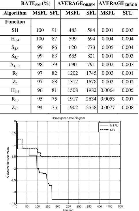
As Table 1 shows, when the search space is more complicated, the rate of successful minimization is decreased. Though, MSFL has better successful minimization than SFL method. This means that MSFL can escape from local minima trap rather than SFL algorithm. MSFL and SFL algorithms, starting from the same point, are compared in Figure 1 for H6,4
function. After 115 iterations, SFL is trapped into a local minimum (0.232, 0.413, 0.830, 0.373, 0.100, 0.999) and the value of function is equal to -1.509, while MSFL algorithm has escaped from local minima (H6,4 function has four local minima) and after
170 iteration has achieved the global minima (0.201, 0.150, 0.476, 0.275, 0.311, 0.675) and the value of function is equal to -3.322. It can be inferred, MSFL possesses escaping property from local optima because of superseding frogs.
[image:3.612.318.559.101.476.2]Comparing the average of the objective function evaluation numbers (Table 1.), as a criterion of algorithm speed, it can be seen that MSFL algorithm is faster than SFL. The high speed of MSFL method is achieved by adding adaptive terms to the position changing formula (Eqs. 3 and 4). Figure 2 shows a typical diagram of two algorithms convergence rates for SH function, starting from the same initial point. It is obvious that although both algorithms can find the optima, MSFL is faster than SFL dramatically. Therefore, in many real world applications that real time computations and less CPU time consumption are needed, MSFL can work better than SFL algorithm. For the successful minimizations, average errors of both algorithms are approximately similar and are less than 0.01, revealing that both algorithms have good accuracies in finding solutions. This accuracy is acceptable for many real world optimization problems. As a conclusion, the results shown in Table 1 indicate that MSFL algorithm not only has great advantage of fast convergence, but also it obtains both better and more robust results over standard SFL algorithm.
Table 1. Results of MSFL and SFL methods for test functions RATESM (%) AVERAGEOBJEN AVERAGEERROR
Algorithm MSFL SFL MSFL SFL MSFL SFL Function
SH 100 91 483 584 0.001 0.003
H3,4 100 87 599 694 0.004 0.004
S4,5 99 86 620 773 0.005 0.004
S4,7 99 83 665 821 0.001 0.003
S4,10 98 79 690 791 0.002 0.003
R5 97 82 1202 1745 0.003 0.001
Z5 97 83 1312 1678 0.002 0.002
H6,4 96 81 1508 1982 0.0064 0.005
R10 95 75 1917 2634 0.0053 0.007
Z10 94 75 1902 2558 0.0077 0.008
Figure 1. Convergence rate of MSFL and SFL algorithms for H6, 4 function
5.
CONCLUSIONS
In this paper, a new modified SFL algorithm (MSFL) was proposed. Two major modifications were accomplished making MSFL possesses excellent properties, i.e., avoiding the premature convergence problem effectively, escaping from local optima, and also having good optimization performance and better diversification ability compared to the standard SFL algorithm. Different benchmarks were used to illustrate the mentioned advantages.
0 50 100 150 200 250 300 350 400 450 500
-3.5 -3 -2.5 -2 -1.5 -1 -0.5 0
Iteration
O
b
je
c
ti
v
e
f
u
n
c
ti
o
n
v
a
lu
e
Convergence rate diagram
[image:3.612.319.560.103.470.2]29
Figure 2. Convergence rate of MSFL and SFL algorithms for SH function
6.
APPENDICES
6.1
Appendix A. The Pseudocode for MSFL
Algorithm
Begin;
1. Set initial values such as size of the population, the number of memeplexes m, random population of P frogs, maximum number of iterations, etc;
2. For each individual calculate objective value;
3. Sort the population P in descending order of their objective values;
4. Divide P into m memeplexes;
5. For each memeplex:
Do:
Sort the frogs in descending order of their objective value;
Determine the best and worst frogs;
Improve the worst frog position using Eq. (4).
Repeat for a specific number of iterations;
End;
6. In each memeplex, replace a frog with another random frog (superseding frog);
7. Combine the evolved memeplexes;
8. Sort the population P in descending order of their objective value;
9. Check if termination condition is true then stop, otherwise go to step 3;
End;
6.2
Appendix B. Some Well-known
Benchmark Functions of Optimization
Problems
6.2.1
Shubert (SH) (2 variables)
SH(x1, x2) =
j
cos[(
j
1
)
x
J
]
51
j
1
×
5j
cos[(
j
1
)
x
J
]
1
j
2
Search domain: -10< xj <10, j=1, 2;
760 local minima;
18 global minimum;
SH((x1, x2)*) = -186.7309;
6.2.2
Hartmann (H3, 4) (3 variables)
H3, 4(x1, x2, x3) =
c
exp[
a
(
x
p
)
]
31 j
2 ij j ij 4
1
j i
;Search domain: 0< xj <1, j=1, 2, 3;
4 local minima: Pi = (pi1, pi2, pi3) = ith local minimum
approximation;
H3, 4 (Pi) -ci;
1 global minimum: X*= (0.11, 0.555, 0.855);
H3, 4 ((x1, x2, x3)*) = -3.86278;
6.2.3
Shekel (S4, n) (3 variables)
S4, n (X) = - i T i i 1
n 1
j
[
(
X
a
)
(
X
a
)
c
]
X = (x1, x2, x3, x4) T
;
ai = ( 1 i
a
,a
i2,a
3i,a
4i )T;3 functions were considered: S4, 5, S4, 7 and S4, 10;
Search domain: 0< xj <10, j=1, 2, 3, 4;
n local minima: ai = ith local minimum approximation;
S4, n (aiT)
-1/ci;1 global minimum for each function;
S4, 5(X) = -10.1532, S4, 7(X) = -10.40294, S4, 10(X) = -10.53641
Table 2. Test function parameters
i ai
T
ci
1 4.0 4.0 4.0 4.0 0.1
2 1.0 1.0 1.0 1.0 0.2
3 8.0 8.0 8.0 8.0 0.2
4 6.0 6.0 6.0 6.0 0.4
5 3.0 7.0 3.0 7.0 0.4
6 2.0 9.0 2.0 9.0 0.6
7 5.0 5.0 3.0 3.0 0.3
8 8.0 1.0 8.0 1.0 0.7
9 6.0 2.0 6.0 2.0 0.5
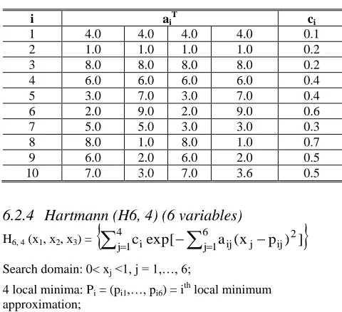
10 7.0 3.0 7.0 3.6 0.5
6.2.4
Hartmann (H6, 4) (6 variables)
H6, 4 (x1, x2, x3) =
c
exp[
a
(
x
p
)
]
61 j
2 ij j ij 4
1
j i
Search domain: 0< xj <1, j = 1,…, 6;
4 local minima: Pi = (pi1,…, pi6) = i th
local minimum approximation;
0 50 100 150 200 250 300 350 400 450 500
-200 -150 -100 -50 0 50
Iteration
O
b
je
c
ti
v
e
f
u
n
c
ti
o
n
v
a
lu
e
Convergence rate diagram
[image:4.612.316.556.491.710.2]30 H6, 4 (Pi)
-ci;1 global minimum: X* = (0.201, 0.150, 0.476, 0.275, 0.311, 0.657);
H6, 4 ((x1, x2, x3)*) = -3.3223;
6.2.5
Rosenbrock (Rn) (n variables)
];
)
1
x
(
)
x
x
(
100
[
)
X
(
R
2j j 1 2 j 2n 1 j
n
Search domain: -5< xj <10, j = 1,…, n;
Several local minima (exact number unspecified in usual literature);
1 global minimum: X* = (1,…, 1);
Rn (X*) = 0;
6.2.6
Zakharov (Zn) (n variables)
n 41 j 2 n
1 j n
1 j
2 j
n
(
x
)
x
(
0
.
5
jxj
)
(
0
.
5
jxj
)
Z
Search domain: -5<xj<10, j = 1, …, n;
Several local minima;
1 global minimum: X* = (1,…, 1);
Zn (X*) = 0;
Table 3. Test function parameters
i aij ci pij
1 3.0 10.0 30.0 1.0 0.3689 0.1170 0.2673
2 0.1 10.0 35.0 1.2 0.4699 0.4387 0.7470
3 3.0 10.0 30.0 3.0 0.1091 0.8732 0.5547
4 0.1 10.0 35.0 3.2 0.0381 0.5743 0.8828
7.
REFERENCES
[1] Z.L. Gaing, A Particle Swarm Optimization Approach for Optimum Design of PID controller in AVR system, IEEE Transactions on Energy Conversion, Vol 9(2), 2003, pp. 384-391.
[2] Z.Y. Zhao, M. Tomizuka, and S. Isaka, Fuzzy gain scheduling of PID controllers, IEEE Trans. System, Man,
and Cybernetics, Vol. 23, No. 5, 1993, pp. 1392-1398.
[3] A. Visioli, Fuzzy logic based set-point weight tuning of PID controllers, IEEE Trans. System, Man, and Cybernetics – Part A: System and Humans, Vol. 29, No. 6, 1999, pp. 587-592.Tavel, P. 2007 Modeling and Simulation Design. AK Peters Ltd.
[4] S.Y. Chu, C.C. Teng, Tuning of PID controllers based on gain and phase margin specifications using fuzzy neural network, Fuzzy Sets and Systems, Vol. 101(1), 1999, pp. 21-30.
[5] G. Zhou and J. D. Birdwell, Fuzzy logic-based PID autotuner design using simulated annealing, Proceedings of the IEEE/IFAC Joint Symposium on Computer-Aided Control System Design, 1994, pp. 67 – 72.
[6] D. P. Kwok and F. Sheng, Genetic algorithm and simulated annealing for optimal robot arm PID control, Proc IEEE Conf. Evolutionary Computation, 1994, pp. 707–713.
[7] R. A. Krohling and J. P. Rey, Design of optimal disturbance rejection PID controllers using genetic algorithm, IEEE Trans. Evol. Comput., Vol. 5, 2001, pp. 78–82,.
[8] P. Wang and D.P. Kwok, Optimal design of PID process controllers based on genetic algorithms, Control Engineer Practice, Vol. 2, No. 4, 1994, pp.641-648.
[9] D. H. Kim, Tuning of a PID controller using a artificial immune network model and local fuzzy set, Proceedings of the Joint 9th IFSA World Congress and 20th NAFIPS International Conference, Vol.5, 2001, pp. 2698 – 2703.
[10]Y.T. Hsiao, C.L. Chuang, and C.C. Chien, Ant colony optimization for designing of PID controllers, Proceedings of the 2004 IEEE Conference on Control Applications/ International Symposium on Intelligent Control/International Symposium on Computer Aided Control Systems Design, Taipei, Taiwan, , 2004.
[11]MM. Eusuf, KE. Lansey, Optimization of water distribution network design using the shuffled frog leaping algorithm. J Water Resour Plan Manage, Vol 129(3), 2003, pp. 210–225.
[12]S. Y. Liong, Md. Atiquzzaman., Optimal design of water distribution network using shuffled complex evolution. J Inst Eng, Singapore, Vol 44(1), 2004, pp. 93–107.
Table 4. Test function parameters
i aij ci pij
1 10.0 3.00 17.0 3.5 1.70 8.00 1.0 0.1312 0.1696 0.5569 0.0124 0.8283 0.5886
2 0.05 10.0 17.0 0.1 8.00 14.0 1.2 0.2329 0.4135 0.8307 0.3736 0.1004 0.9991
3 3.00 3.50 1.70 10 17.0 8.00 3.0 0.2348 0.1451 0.35522 0.2883 0.3047 0.6650