PSO based Optimum Design of PID Controller for Mobile Robot Trajectory Tracking

PSO-based Optimum Design of PID Controller for Mobile

Robot Trajectory Tracking

Turki Y. Abdalla

Department of Computer Engineering University of Basrah

Basrah,Iraq

Abdulkareem. A. A

Department of Electrical Engineering University of Basrah

Basrah,Iraq

ABSTRACT

This paper present a particles swarm optimization (PSO) method for determining the optimal proportional – integral derivative (PID) controller parameters, for the control of nonholonomic mobile robot that involves path tracking using two optimized PID controllers one for speed control and the other for azimuth control. The mobile robot is modelled in Simulink and PSO algorithm is implemented using MATLAB. Simulation results show good performance for the proposed control scheme.

Keywords

Mobile Robot, Particles Swarm Optimization, PID Controller, Kinematic and dynamic model,Trajectory tracking.

1.

INTRODUCTION

Autonomous robots may act instead of human beings. The robots are able to accomplish many tasks in dangerous places where humans cannot enter, such sites where harmful gases or high temperature are present a hard environment for humans. Cleaning robots and cargo delivery can work automatically and save costs by performing various routine tasks [1,2]. This means that it is needed to evolve robot controllers that solve complicated problems and tackle complicated in the variable environments. There are several types of controllers that used for control the mobile robot the simplest one is PID controller.

The PID controller has been used to control about 90% of industrial processes worldwide [3]. The main problem of that simple controller is the correct choice of the PID gains and the fact that by using fixed gains, the controller may not provide the required control performance, when there are variations in the plant parameters and operating conditions. Therefore, a tuning process must be performed to insure that the controller can deal with the variations in the plant [4]. To tune the PID controller, there are numbers of strategies, the most famous, which is frequently used in industrial applications, is the Ziegler-Nichols method [3] , genetic algorithm GA, etc. Moreover, PSO was another method for tuning procedure. PSO first introduced by Kennedy and Eberhart is one of the modern heuristic algorithms, it has been motivated by the behavior of organisms, such as fish schooling and bird flocking [5]. Generally, PSO is characterized as a simple concept, easy to implement, and computationally efficient. Unlike the other heuristic techniques, PSO has a flexible and well-balanced mechanism to enhance the global and local exploration abilities [6]. In this paper, a novel PSO-based approach to optimally design a PID controller for a mobile robot trajectory tracking is proposed. This paper has been organized as follows: in section 2 both kinematics and dynamic models of mobile robot are described. In section 3, the particle swarm optimization method is reviewed. Section 4, describes how PSO is used to design t`he PID controller optimally for mobile robot to control the velocity and

azimuth. The simulation and the results are presented in section 5.

2.

A

NONHOLONOMIC

MOBILE

ROBOT

MODEL

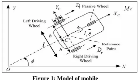
A mobile robot is located in a two dimensional Cartesian workspace, in which a global coordinate {X, 0, Y}is defined. A local coordinate {𝑋𝑐, C, 𝑌𝑐} is attached to the robot with the origin at point C, the middle points of two wheels which is the guide point of this mobile robot. A typical mobile robot model is shown in Figure 1, where b is the half distance between two wheels. There are several ways to set up a steering system for differential drive mobile robot. A robot must have a minimum of three wheels in order to work.

[image:1.595.321.554.468.602.2]

All the combinations require two motorized wheels and at least one swiveling wheel for balance [7]. Consider the mobile robot depicted in Figure 1 as front drive used in this paper. The platform moves by driving the two independent wheels as shown in the Figure 1. We assume that the speed at which this system moves is low and therefore the two driven wheels do not slip sideways.

Let us consider the kinematic model (study of the mathematics of motion without considering the forces that affect the motion , it deals with the geometric relationships that govern the system and deals with the relationship between control parameters and the behavior of a system in state space [8]) for an autonomous vehicle. The position of the mobile robot in the plane is shown in Figure 1, the inertial-based frame (Oxy) is fixed in the plane of motion and the moving frame is attached to the mobile robot. The mobile robots are rigid cart equipped, with non-deformable conventional wheels, and it is moving on a non-deformable horizontal plane. During the motion: the contact between the wheel and the horizontal plane is reduced to a single point, the wheels are fixed, the plane of each wheel remains vertical, the wheel rotates about its horizontal axle and the orientation of the horizontal axle with respect to the cart can be fixed [9]. This means that the velocity of the contact point between each wheel and the horizontal plane is

Figure 1: Model of mobile

robot mmmmobile mobile robot

equal to zero. The rotation angle of the wheel about its horizontal axle is denoted by φ(t) and the radius of the wheel by r. Hence, the position of the wheel is characterized by two constants: b and r

and its motion by: φr(t) – the rotation angle of the right wheel and φl(t) – the rotation angle of the left wheel. The configuration of the

mobile robot can be described by five generalized coordinates (q) such as [9, 10]:

)

,

,

,

(

x

c,

y

c r l

q









(1)

where: xc and yc are the two coordinates of the origin C of the moving frame (the geometric center of the mobile robot), θ is the orientation angle of the mobile robot (of the moving frame). The vehicle velocity v can be found in Equation (2) [3, 5, 6]: 𝑣 =𝑅(𝑤𝑟+𝑤𝑙) 2 (2)

where: 𝑤𝑟=𝑑𝜑_𝑑𝑡𝑟 (Angular velocity of the right wheel) 𝑤𝑙=𝑑𝜑_𝑑𝑡𝑙 (Angular velocity of the left wheel) The position and the orientation of the mobile robot are determined by a set of differential equations in the following forms [7, 3 ,6, 8]: 𝑥 = (𝑅 𝑐𝑜𝑠𝜃 𝑤𝑟+ 𝑤𝑙 )/2 (3)

𝑦 = (𝑅 𝑠𝑖𝑛𝜃 𝑤𝑟+ 𝑤𝑙 )/2 (4)

𝜃 = 𝑅(𝑤𝑟+ 𝑤𝑙)/2𝑏 (5)

Here, 𝑥 = 𝑣 𝑐𝑜𝑠𝜃, 𝑦 = 𝑣 𝑠𝑖𝑛𝜃 Finally, the kinematics model of the vehicle velocity v and the orientation θ can be represented by the matrix as follows [9 ]: 𝑣 𝜃 = 𝑅/2𝑏 −𝑅/2𝑏 𝑅/2 𝑅/2 𝑤𝑟 𝑤𝑙 (6)

A large number of researchers have used kinematic models to develop motion control strategy for mobile robots, their assumption that these models are valid if the robot has low speed, low acceleration and light load [10]. Dynamic modeling takes into account the forces acting on the vehicle. This model can be constructed using the no-slip condition [11] or allowing wheel slip [12]. In either case, the acceleration is considered. In dynamic modeling the vehicle‟s dynamic properties, such as mass, center of gravity, etc. are entered into the equations. To drive this model, the nonholonomic constraints of the system are utilized .Dynamic equation of wheeled mobile robot is described as[13]: M(q)𝑤 +C(𝑞, 𝑞 )𝑤+Dw=τ (7)

(8)

(9)

(10)

(11)

(12)

(13)

𝐷 = 𝑑11_{0 𝑑22}0 (14)

(15)

𝑤 = 𝜃 = 𝑑𝜃/𝑑𝑡 (16)

𝑤𝑟 𝑤𝑙: are angular velocities of right and left wheel respectively. 𝑚𝑐 : is the mass of body. 𝑚𝑤: is the mass of the wheel with a motor. 𝐼𝑐: the moment of inertia of the body about vertical axis through the center of mass. 𝐼𝑤: is the moment of inertia of the wheel with a motor about the wheel diameter . R: is the radius of the wheel. a: is the distance between the robot‟s center of mass and the center of the wheel axle. b: is the half distance between the two wheels. 𝑑11, 𝑑22: are damping coefficients. q=(x, y, θ): is the vector of generalized coordinates. τ=[τ𝑣 τ𝑤]: is the vector of torque applied to the wheels of the robot. M(q); is 2*2 positive-definite inertia matrix. From the above equation we can get, (17)

3. OVERVIEW OF PARTICLE SWARM

OPTIMIZATION

Particle Swarm Optimization (PSO) is a technique used to explore the search space of a given problem to find the settings or parameters required to maximize a particular objective. This technique, first described by James Kennedy and Russell C. Eberhart in 1995 [14]. PSO is one of the optimization techniques and a kind of evolutionary computation technique. The method has been found to be robust in solving problems featuring nonlinearity and non differentiability, multiple optima, and high dimensionality through adaptation, which is derived from the social-psychological theory [15]. The technique is derived from research on swarm such as fish schooling and bird flocking. According to the research results for a flock of birds, birds find food by flocking (not by each individual). The observation leads the assumption that every information is shared inside flocking. Moreover, according to observation of behavior of human groups, behavior of each individual (agent) is also based on behavior patterns authorized by the groups such as customs and other behavior patterns according to the experiences by each individual. The assumption is a basic concept of PSO [16]. In the PSO algorithm, instead of using

M(q)= 𝑚_𝑚11 𝑚12

12 𝑚11 𝑤 = [𝑤𝑟𝑤𝑙] , τ=[τ𝑣τ𝑤]

m=𝑚𝑐 +2𝑚𝑤

I=𝑚_𝑐𝑎2+2𝑚_𝑤𝑏2+𝐼_𝑐+2𝐼_𝑚

𝑚 = 0.25𝑏−2_𝑟2_(m𝑏2_+I)+𝐼

𝑚12= 0.25𝑏−2𝑟2(m𝑏2-I)

C(q,𝑞 )= 0 𝑐𝜃

−𝑐𝜃 0

evolutionary operators such as mutation and crossover, to manipulate algorithms, for a d-variables optimization problem, a flock of particles are put into the d-dimensional search space with randomly chosen velocities and positions knowing their best values so far (Pbest) and the position in the d-dimensional space. The velocity of each particle, adjusted according to its own flying experience and the other particle‟s flying experience. For example, the 𝑖𝑡𝑕 particle is represented as 𝑥𝑖= 𝑥𝑖,1, 𝑥𝑖,2, … , 𝑥𝑖,𝑑 in the

d-dimensional space. The best previous position of the i th particle is recorded and represented as:

𝑃𝑏𝑒𝑠𝑡𝑖= (𝑃𝑏𝑒𝑠𝑡𝑖,1, 𝑃𝑏𝑒𝑠𝑡𝑖,2, … , 𝑃𝑏𝑒𝑠𝑡𝑖,𝑑)

The index of best particle among all of the particles in the group is 𝑔𝑏𝑒𝑠𝑡𝑑. The velocity for particle i is represented as

𝑣𝑖= (𝑣𝑖,1, 𝑣𝑖,2, … , 𝑣𝑖,𝑑) The modified velocity and position of each particle can be calculated using the current velocity and the distance from 𝑃𝑏𝑒𝑠𝑡𝑖,𝑑 to 𝑔𝑏𝑒𝑠𝑡𝑖,𝑑 as shown in the following formulas[15]:

𝑣𝑖,𝑚𝑡+1= 𝑤. 𝑣𝑖,𝑚𝑡 + 𝑐1∗ 𝑅𝑎𝑛𝑑 ∗ 𝑝𝑏𝑒𝑠𝑡𝑖,𝑚− 𝑥𝑖,𝑚 𝑡 + 𝑐2∗

𝑟𝑎𝑛𝑑 ∗ (𝑔𝑏𝑒𝑠𝑡𝑚−) (18)

𝑥_𝑖,𝑚(𝑡+1)= 𝑥_𝑖,𝑚(𝑡)+ 𝑣_𝑖,𝑚(𝑡+1) (19)

𝑖 = 1,2, … , 𝑛 ; 𝑚 = 1,2, … , 𝑑 where

𝑛 Number of particles in the group.

𝑑 Dimension.

𝑡 Pointer of iteration (generations).

𝑣_𝑖,𝑚(𝑡) Velocity of particle 𝑖 at iteration t

𝑣𝑑𝑚𝑖𝑛 ≤ 𝑣𝑖,𝑑 (𝑡)

≤ 𝑣𝑑𝑚𝑎𝑥. 𝑤 Inertia weight factor.

𝑐1, 𝑐2 Acceleration constant.

Rand(),rand() Random number between 0 and 1.

𝑥_𝑖,𝑑(𝑡) Current position of particle I at iterations.

𝑃𝑏𝑒𝑠𝑡𝑖 Best previous position of the ith particle.

𝑔𝑏𝑒𝑠𝑡 Best particle among all the particle in the Population.

4. IMPLEMENTATION OF PSO-PID

CONTROLLER

4.1

Fitness Function

Unit

In PID controller design methods, the most common performance criteria are integrated absolute error (IAE), the integrated of time weight square error (ITSE), integrated of squared error (ISE) and Mean Square Error (MSE) [17, 18]. These four integral performance criteria have their own advantages and disadvantages. For example, disadvantage of the IAE and ISE criteria is that its minimization can result in a response with relatively small overshoot but a long settling time because the ISE performance criterion weights all errors equally independent of time. Although the ITSE performance criterion can overcome the disadvantage of

the ISE criterion, the derivation processes of the analytical formula are complex and time-consuming [18]. The IAE , ISE , ITSE , and MSE performance criterion formulas are as follows:

a) Integral of Absolute Magnitude of the Error (IAE) 𝐼𝐴𝐸𝑇𝑜𝑡𝑎𝑙 = ( 𝑒𝜃₀∞ 𝑑𝑡)+ ( 𝑒𝑣 𝑑𝑡)₀∞ (20)

b) Integral of the Square of the Error (ISE)

𝐼𝑆𝐸𝑇𝑜𝑡𝑎𝑙 = ( 𝑒𝑣₀∞ 𝑡 2𝑑𝑡)+ ( [𝑒𝜃₀∞ (𝑡)]2𝑑𝑡) (21)

c) Integral of Time multiplied by Absolute Error (ITAE) 𝐼𝑇𝐴𝐸𝑡𝑜𝑡𝑎𝑙 = ( 𝑡|𝑒𝜃₀∞ (𝑡)|𝑑𝑡) + ( 𝑡|𝑒𝑣 𝑡 |𝑑𝑡) ₀∞ (22)

d) Mean Square Error (MSE) 𝑀𝑆𝐸𝑡𝑜𝑡𝑎𝑙 = 1_𝑛 𝑛 𝑒𝜃 𝑘 2

𝑘=1 + _𝑛1 𝑒𝑣 𝑘 2 𝑛

𝑘=1 (23)

n: represents number of samples, k: sample time.

In this paper a time domain criterion is used for evaluating the PID controller [15]. A set of good control parameters P,I and D can yield a good step response that will result in performance criteria minimization in time domain. In this paper we‟ll use Equation ( 23) as a fitness function.

3.2

Proposed PSO-PID Controller

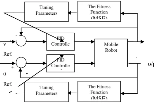
In this paper the PSO algorithm is used to find the optimal parameters for two PID controllers for the control of velocity and azimuth of mobile robot . Figure 2 shows the block diagram of optimal PID controller for the mobile robot.

In the proposed PSO method each particle contains six members 𝑃1, 𝐼1 and 𝐷1 (parameters of velocity controller), 𝑃2 , 𝐼2

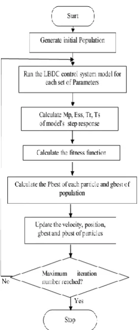
and 𝐷2 (parameters of azimuth controller). The search space has six dimension and particles must „fly‟ in six dimensional space. The flowchart of PSO-PID controller is shown in Figure 3.

v Ref.

θ Ref.

[image:3.595.321.573.471.641.2]

Figure 2: Optimal PID controller +

-- +

Mobile Robot PID

Controlle r1

The Fitness Function (MSE) Tuning

Parameters

PID Controlle

r2

The Fitness Function (MSE) Tuning

Parameters

--

o/p

[image:4.595.110.251.65.402.2]

Figure 3: Flowchart of the PSO-PID Control System

Table 1: The physical parameters of mobile robot

Parameter Value Unit

R 0.15 M

B 0.75 M

A 0.3 M

𝑚𝑐 30 Kg

𝑚𝑤 1 Kg

𝐼𝑐 15.625 Kg. 𝑚2

𝐼𝑤 0.005 Kg. 𝑚2

𝐼𝑚 0,0025 Kg. 𝑚2

𝑑11 10 _

𝑑22 10 _

C 0.135 _

5. SIMULATION AND RESULTS

I

n order to build the mobile robot given by Equation (17) , the values of physical parameters shown in Table 1 are used [13]. By several experiment , the following PSO parameters are used to obtain the optimal performance of the controller :

Wmax=0.9 , Wmin=0.4; 𝑐1= 𝑐2= 1.2 ;

By doing several experiment using different values for population size and number of iterations .The following values for them are considered to be acceptable.

Population size=30; Number of iteration =40.

The result obtained in 40 iterations as shown in Table 2:

Table2:Parameters of PID controllers optimized by PSO

𝑃1 𝐼1 𝐷1 𝑃2 𝐼2 𝐷2

214.3 533.3 257 357.9 403.7 176

These values are considered as parameters of the two optimal PID controllers that give the lowest MSE. The system is tested for three different cases as follows :

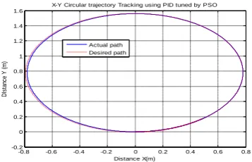
1) The desired circular trajectory given by a reference velocity

𝑣𝑑 of 1 [meter/sec] and a reference azimuth 𝜃𝑑 given as :

𝜃𝑑 =[(2 ∗ 𝜋)/𝑚 × 𝑓(𝑡)[𝑟𝑎𝑑] where 𝑚 (slop) = 0.1592, 𝑓 𝑡 = 𝑡, 0 ≤ 𝑡 ≤ 7

[image:4.595.350.524.366.479.2]

Figure 4 shows the velocity error, Figure 5 shows the azimuth error, Figure 6 shows the actual and desired path for circular trajectory . The MSE= 0.000095.

Figure 4: The error in velocity

Figure 5: The error in azimuth

0 1000 2000 3000 4000 5000 6000

-2 -1.5 -1 -0.5 0 0.5 1 1.5 2

The Velocity Error

Time (msec)

E

rro

r

0 1000 2000 3000 4000 5000 6000

-2 -1.5 -1 -0.5 0 0.5 1 1.5 2

The Azimuth error

Time (msec)

Er

ro

Figure 6: circular trajectory tracking using PSO-PID controller

2) To follow a desired square trajectory.

[image:5.595.79.258.71.186.2] [image:5.595.256.543.87.688.2]

Figure 7 shows the desired and actual square trajectory Figure 8 shows the error in azimuth and Figure 9 shows the error in velocity . The MSE= 0.00055

Figure 7: square trajectory tracking using PSO-PID controllers

Figure 8: The error in velocity

Figure 9: The error in azimuth

3) To follow a desired sine trajectory.

Figure 10 shows the desired and actual sine trajectory Figure 11 shows the error in azimuth and Figure 12 shows the error in velocity . The MSE= 0.000085. Table 3 shows the values of MSE in all cases.

Table 3: MSE for different trajectories

Trajectory Circular Square Sine MSE 0.000095 0.00055 0.000085

[image:5.595.79.260.308.412.2]

Figure10: Sine trajectory tracking using PSO-PID controllers

[image:5.595.78.260.338.703.2]

Figure 11 : Error in azimuth for sine trajectory tracing

Figure 12: Error in velocity for sine trajectory tracking

6.

CONCLUSION

PSO-PID controller is built and implemented in matlab / simulink software package and it is succeeded to solve the trajectory tracking problem in mobile robot . The Particle Swarm Optimization method is utilized to tune/optimize the parameters of PID controller and its gives us a good results in short time relatively with other optimization methods. Simulation results show good tracking performance with small Mean square error. The resulting good tracking capability and small MSE values show that the proposed method is more effective than other methods such as Ziegler-Nichols method and genetic algorithm approach.

7.

REFERENCES

[1] Y. Shinoda, Y. Tan, J. Nakata and R. Beuran ,"Collaborative Motion Planning of Autonomous Robots", School of Information Science, Japan Advanced Institute of Science and Technology, Ishikawa Japan, 2007.

[2] R. A. Felder , "Mobile Robot Simulation of Clinical Laboratory Deliveries", M.Sc. Thesis, the University of Virginia, U.S.A, 1998.

-0.8 -0.6 -0.4 -0.2 0 0.2 0.4 0.6 0.8 -0.2 0 0.2 0.4 0.6 0.8 1 1.2 1.4 1.6 Distance X(m) D Is ta nc e Y ( m )

X-Y Circular trajectory Tracking using PID tuned by PSO

Actual path Desired path

-0.5 0 0.5 1 1.5 2 2.5

-0.5 0 0.5 1 1.5 2 2.5

Distance X (m)

D is ta nc e Y (m )

X-Y square trajectory tracking using PID controller tuned by PSO Actual path Desired path

0 1000 2000 3000 4000 5000 6000

-2 -1.5 -1 -0.5 0 0.5 1 1.5 2

The Velocity Error

Time (msec)

E

rro

r

0 1000 2000 3000 4000 5000 6000

-2 -1.5 -1 -0.5 0 0.5 1 1.5 2

The Azimuth error

Time (msec)

Er

ro

r

0 1 2 3 4 5 6 7

-0.2 0 0.2 0.4 0.6 0.8 1 1.2 1.4 1.6 1.8

Distanc X (m)

D is ta nc e Y ( m )

X-Y sin trajectory tracking by usin PID controllers tuned by PSO actual path desired path

0 1 2 3 4 5 6 7 8

-2 -1.5 -1 -0.5 0 0.5 1 1.5 2 Time (sec) E rro r Azimuth Error

0 1 2 3 4 5 6 7 8

[image:5.595.342.526.414.505.2]

[3] A. Haj-Ali and H. Ying , "Structural Analysis of Fuzzy Controllers with Nonlinear Input Fuzzy Sets in Relation to Nonlinear PID Control with Variable Gains", Associate Editor Gary G. Yen under the direction of Editor Robert R. Bitmead, Wayne State University , Detroit , MI48202 ,USA ,2004, available on the following link: www.sciencedirect.com.

[4] S. M. Gadoue, D. G. and J. W. Finch, "Tuning of PI Speed Controller in DTC of Induction Motor Based on Genetic Algorithms and Fuzzy Logic Schemes", International Journal of Advanced Robotic Systems, University of Newcastle upon Tyne, pp.187 - 194, ISSN 1229-3406, 2005. [5] J. Kennedy and R. Eberhart, “Particle swarm optimization,” in Proc. IEEE Int. Conf. Neural Networks , vol. IV, Perth, Australia, 1995, pp. 1942–1948.

[6] M. A. Abido, “Optimal design of power-system stabilizers using particleswarm optimization,” IEEE Trans. Energy Conversion, vol. 17, pp.406-413, Sep. 2002.

[7] D. R. Shircliff, "Build A Remote-Controlled Robot", eBook, Copyright © by The McGraw-Hill Companies, 2002. [8] . ] M. I. Ribeiro and P. Lima, "Kinematics Models of Mobile

Robots", Av. Rovisco Pais, 11049-001 Lisboa, April, 2002 [9] G. Mester, "Obstacle Avoidance of Mobile Robots in

Unknown Environments", SISY, International Symposium on Intelligent Systems and Informatics 24-25 Subotica, Serbia, August, 2007.

[10]A. Albagul and Wahyudi, "Dynamic Modelling and Adaptive Traction Control for Mobile Robots", 30th Annual Conference of the IEEE Industrial Electronics Society, November 2 - 6, Susan, Korea 2004.

[11]E.N.moret, “Dynamic modeling and control of a car-like robot”Master‟s thises, Virginia Polytechnic Institute and state University ,2003.

[12]P.Kachoor and M.tomizuka, “vehicle control for automated highway systems for improve lateral maneuverability,” in IEEE International conference on systems,Man, and Cybernetics , Vancouver ,B.C., Canada , vol. 1,pp.777-782, Oct. 1995.

[13]Duc Do,K.,Zhong-Ping j.,Pan,J.”A global output-feedback controller for simultaneous tracking and stabilization of unicycle-type mobile robots,” IEEE Trans. Automat Contr., V30,N3,pp. 589-594, 2004.

[14]J. Kennedy and R. Eberhart, “Particle swarm optimization,” in Proc.IEEE Int. Conf. Neural Networks , vol. IV, Perth, Australia, 1995,pp.1942–1948.

[15]Z.-L. Gaing, “A particle swarm optimization approach for optimum design of PID controller in AVR system,” IEEE Trans. EnergyConversion, vol. 19, pp. 384-391, June 2004. [16]H. Yoshida, K. Kawata, Y. Fukuyama, S. Takayama, and Y. Nakanishi, “A particle swarm optimization for reactive power and voltage control considering voltage security assessment,” IEEE Trans. on Power Systems, Vol. 15, No. 4, Nov. 2000, pp. 1232 – 1239.

[17]R. A. Krohling and J. P. Rey, “Design of optimal disturbance rejectionPID controllers using genetic algorithm,” IEEE Trans. Evol.Comput.,vol. 5, pp. 78–82, Feb. 2001.

[18]R. A. Krohling and J. P. Rey, “Design of optimal disturbance rejectionPID controllers using genetic algorithm,” IEEE Trans. Evol. Comput.,vol. 5, pp. 78–82, Feb. 2001.