BIROn - Birkbeck Institutional Research Online
Wojtys, Małgorzata and Marra, Giampiero and Radice, Rosalba (2018)
Copula based generalized additive models for location, scale and shape with
non-random sample selection. Computational Statistics and Data AnalysiS
127 , pp. 1-14. ISSN 0167-9473.
Downloaded from:
Usage Guidelines:
Please refer to usage guidelines at or alternatively
Copula based generalized additive models for location, scale and shape with
non-random sample selection
Małgorzata Wojty´sa,, Giampiero Marrab, Rosalba Radicec aCentre for Mathematical Sciences, University of Plymouth bDepartment of Statistical Science, University College London cDepartment of Economics, Mathematics and Statistics, Birkbeck
Abstract
Non-random sample selection is a commonplace amongst many empirical studies and it appears when an output variable of interest is available only for a restricted non-random sub-sample of data. An extension of the generalized additive models for location, scale and shape which accounts for non-random sample selection by introducing a selection equation is discussed. The proposed approach allows for potentially any parametric distribution for the outcome variable, any parametric link function for the selection equation, several dependence structures between the (outcome and selection) equations through the use of copulae, and various types of covariate effects. Using a special case of the proposed model, it is shown how the score equations are corrected for the bias deriving from non-random sample selection. Parameter estimation is carried out within a penalized likelihood based framework. The empirical effectiveness of the approach is demonstrated through a simulation study and a case study. The models can be easily employed via thegjrm()function in theRpackageGJRM.
Keywords: additive predictor, copula, marginal distribution, non-random sample selection, penalized regression
spline, simultaneous equation estimation.
1. Introduction
Non-random sample selection arises when an output variable of interest is available only for
a restricted non-random sub-sample of the data. This often occurs in sociological, medical and
economic studies where individuals systematically select themselves into (or out of) the sample
(e.g., Lennox et al., 2012; Vella, 1998; Collier and Mahoney, 1996, and references therein). If the
aim is to model an outcome of interest in the entire population and the link between its availability
in the sub-sample and its observed values is through factors which can not be accounted for then
any analysis based on the available sub-sample will most likely lead to biased conclusions.
Sam-ple selection models allow one to use the entire samSam-ple whether or not observations on the output
variable were generated. In its classical form, it consists of two equations which model the
prob-ability of inclusion in the sample and the outcome variable through a set of available covariates,
and of a joint bivariate distribution linking the two equations.
The sample selection model was first discussed by Gronau (1974) and Lewis (1974). Heckman
(1976) formulated a unified approach to estimating this model using a simultaneous equation
system. In the classical version, the error terms of the two equations are assumed to follow a
bivariate normal distribution where non-zero correlation indicates the presence of non-random
sample selection. Heckman (1979) then translated the issue of sample selection into an omitted
variable problem and proposed a simple and easy to implement estimation method known as
two-step procedure.
Various modifications and generalizations of the classical sample selection model have been
proposed in the literature and here we mention some of them. A non-parametric two-stage
ap-proach, which lifts the normality assumption, can be found in Das et al. (2003). Non-parametric
methods are also considered in Lee (2008) and Chen and Zhou (2010). Semi-parametric
ap-proaches can instead be found in Gallant and Nychka (1987), Lee (1994), Powell (1994) and
Newey (2009). In the Bayesian framework, Chib et al. (2009) dealt with non-linear covariate
effects using Markov chain Monte Carlo estimation techniques and simultaneous equation
sys-tems. Wiesenfarth and Kneib (2010) further extended this approach by introducing a Bayesian
algorithm based on low rank penalized B-splines for non-linear and varying-coefficient effects and
Markov random-field priors for spatial effects. Frequentist counterparts of these Bayesian methods
are given in Marra and Radice (2013b) in the context of binary responses and Marra and Radice
(2013a) for continuous Gaussian outcomes. Zhelonkin et al. (2016) introduced a procedure for
robustifying the Heckman’s two stage estimator by using M-estimators of Mallows’ type for both
stages. Marchenko and Genton (2012) and Ding (2014) considered a bivariate Student-t
distribu-tion for the model’s errors as a way of tackling heavy-tailed data. Several authors proposed using
copulae to model the joint distribution of the selection and outcome equations; see, e.g., Prieger
(2002) who employed a Farlie-Gumbel-Morgenstern (FGM) bivariate copula. A more general
copula approach, with a focus on Archimedean copulae, can be found in Smith (2003). As
em-phasized for instance by Genius and Strazzera (2008), copulae allow for the use of non-Gaussian
distributions and have the additional benefit of making it possible to specify the marginal
distribu-tions independently of the dependence structure linking them. Importantly, while the copula
ap-proach is fully parametric, it is typically computationally more feasible than non/semi-parametric
approaches and it still allows one to assess the sensitivity of results to different modeling
assump-tions. The aim of this work is to continue this stream of research.
In this paper, we introduce a generalized additive model for location, scale and shape (GAMLSS,
clas-sical GAMLSS is extended by introducing an extra equation which models the selection process.
Specifically, the selection and outcome equations are linked by a joint probability distribution
which is expressed in terms of a copula. Moreover, using the developments available in the spline
literature (e.g., Ruppert et al., 2003; Wood, 2017), we model the relationship between covariates
and responses by using penalized regression splines, thus capturing possibly complex
relation-ships. Second, we show how the score equations are corrected for the bias deriving from
non-random sample selection. To the best of our knowledge, this aspect has never been elucidated
in the literature and provides an interesting insight into the correction mechanism underlying the
selection approach. Third, we make the new developments available via the gjrm() function
from theRpackageGJRM(Marra and Radice, 2018).
Note that the approach to estimating sample selection models using copulae and penalized
re-gression splines has recently been adopted by Wojty´s et al. (2016), Marra and Wyszynski (2016),
Wyszynski and Marra (2017) and Marra et al. (2017). The former only considers a Gaussian
out-come, whereas the latter works deal with the cases of binary and discrete outcome distributions.
This paper is concerned with providing a general modeling framework where any parametric link
function and continuous distribution for the outcome can be utilized.
The remainder of the paper is organized as follows. Section 2 discusses the proposed sample
selection GAMLSS as well as a special case which elucidates the nature of the non-random sample
selection correction. Section 3 provides some estimation and inferential details. The finite-sample
performance of the approach is investigated in Section 4, whereas a case study is presented in
Section 5.
2. Sample selection GAMLSS
The proposed generalized additive sample selection model for location, scale and shape is
structured as follows. We first assume that the outcome variable of interest can be described by a
GAMLSS (Rigby and Stasinopoulos, 2005). Then, in order to take the selection process into
ac-count, we extend the model by adding the so-called selection equation, which is specified in terms
of a binary regression that makes use of an arbitrary parametric link function. The two equations
are linked by using a bivariate copula. Finally, all parameters of the marginal distributions as well
as copula are specified as flexible functions of covariates.
2.1. Model definition
LetY2∗ denote the random variable of primary interest whose values are observed only for a
that governs the selection process. The observed variables are
Y1 = (Y1∗ >0),
Y2 = Y2∗Y1,
where symbol (·)denotes throughout an indicator function. Random variableY1indicates whether
the value ofY∗
2 is observed. VariableY2 holds the observed value ofY2∗ and equals0 if the
ob-served value is missing.
LetF1(y1∗|θ1)andF2(y∗2|θ2)denote the cumulative distribution functions of the latent
selec-tion variableY∗
1 and of the output variable of interestY2∗, which depend on vectors of parameters
θ1 ∈ Rp1 and θ2 ∈ Rp2, respectively, where p1, p2 ∈ N. Analogically, f1(y∗1|θ1)and f2(y∗2|θ2)
denote the probability (density) functions ofY∗
1 andY2∗. We specify the dependence structure
be-tween the two variables by taking advantage of Sklar’s theorem (Sklar, 1959). It states that for any
two random variables there exists a two-place function, called copula, which represents the joint
cumulative distribution function of the pair in a manner which makes a clear distinction between
the marginal distributions and the form of dependence between them. An exhaustive introduction
to copula theory can be found in Nelsen (2006) and Schweizer (1991). We use the symbolCθ3(·,·)
throughout to denote a copula parametrized withθ3 ∈Rp3, wherep3 ∈N.
LetCθ3(·,·)be the copula such that the joint cdf of(Y1∗, Y2∗)equals
F(y1∗, y2∗|θ1,θ2,θ3) =Cθ3(F1(y∗1|θ1), F2(y2∗|θ2)). (2.1)
FunctionCθ3 always exists and is unique for every(y1∗, y2∗)in the support of the joint distribution F. It is assumed that the unknown parameter vectorsθ1 ∈ Rp1, θ2 ∈ Rp2 andθ3 ∈ Rp3 can be
linked to predictors (containing regression coefficients and covariates) via known monotonic link
functionsg1,j(·),g2,j(·)andg3,j(·)such that fork = 1,2,3it holds that
gk,j(θk,j) = η(k,j) forj = 1, . . . , pk,
where the θk,j are the components of the vectors θk, i.e. θk = (θk,j)j=1,...,pk. The predictors
η(k,j) are assumed to depend on sets of covariates x(k,j), so that η(k,j) = η(k,j)(x(k,j)), where
x(k,j)= (x1(k,j), . . . , x(Dk,jk,j)). More details are given in Section 2.3.
The usual characterization of the GAMLSS model is achieved, for instance, by settingθ1 =
(µ1, σ1, ν1) and θ2 = (µ2, σ2, ν2), where µk, σk and νk, for k = 1,2, represent the parameters
Copula C(u, v;θ3) Range ofθ3 Link Kendall’sτ
AMH ("AMH") 1 uv
−θ3(1−u)(1−v) θ3∈[−1,1] tanh
−1(θ
3) − 2 3θ2
3
θ3+ (1−θ3)2
log(1−θ3)}+ 1
Clayton ("C0") u−θ3+v−θ3−1−1/θ3
θ3∈(0,∞) log(θ3) θ3θ+23
FGM ("FGM") uv{1 +θ3(1−u)(1−v)} θ3∈[−1,1] tanh−1(θ3) 29θ3
Frank ("F") −θ−
1
3 log{1 + (exp{−θ3u} −1)
(exp{−θ3v} −1)/(exp{−θ3} −1)}
θ3∈R\ {0} − 1−θ43[1−D1(θ3)]
Hougaard ("HO") exp
"
−
(−logu) 1
θ3 + (−logv) 1
θ3
θ3#
θ3∈(0,1) log
θ
3
1−θ3
1−θ3
Gaussian ("N") Φ2 Φ−1(u),Φ−1(v);θ3 θ3∈[−1,1] tanh−1(θ3) 2πarcsin(θ3)
Gumbel ("G0") exp
−
(−logu)θ3 +(−logv)θ3 1/θ3
i θ3∈[1,∞) log(θ3−1) 1− 1
θ3
Joe ("J0") 1−
(1−u)θ3+ (1−v)θ3
−(1−u)θ3(1−v)θ3 1/θ3 θ3∈(1,∞) log(θ3−1) 1 +
4 θ2
3 D2(θ3)
Plackett ("PL")
Q−√R/{2(θ3−1)} θ3∈(0,∞) log(θ3) −
Student-t ("T") t2,ζ
t−1
ζ (u), t− 1 ζ (v);ζ, θ3
θ3∈[−1,1] tanh−1(θ3) 2πarcsin(θ3)
Table 1: Definition of copulae implemented inGJRM, with corresponding parameter range of association parameterθ3, link function ofθ3, and
relation between Kendall’sτandθ3.Φ2(·,·;θ3)denotes the cumulative distribution function (cdf) of a standard bivariate normal distribution with
correlation coefficientθ3, andΦ(·)the cdf of a univariate standard normal distribution. t2,ζ(·,·;ζ, θ3)indicates the cdf of a standard bivariate
Student-t distribution with correlationθ3and fixedζ∈(2,∞)degrees of freedom, andtζ(·)denotes the cdf of a univariate Student-t distribution
withζdegrees of freedom.D1(θ3) = θ13
Rθ3
0 exp(tt)−1dtis the Debye function andD2(θ3) =
R1
0 tlog(t)(1−t)
2(1−θ3)
θ3 dt. QuantitiesQand
Rare given by1 + (θ3−1)(u+v)andQ2−4θ3(θ3−1)uv, respectively. The Kendall’sτfor"PL"is computed numerically as no analytical
expression is available. ArgumentBivDofgjrm()inGJRMallows the user to employ the desired copula function and can be set to any of the values within brackets next to the copula names in the first column; for example,BivD = "J0". For Clayton, Gumbel and Joe, the number after the capital letter indicates the degree of rotation required: the possible values are0,90,180and270.
p1 and p2 of population parameters. The distributions for Y2∗ implemented for this work in the
R package GJRM are the normal ("N"), log-normal ("LN"), Gumbel ("GU"), reverse Gumbel
("rGU"), logistic ("LO"), Weibull ("WEI"), inverse Gaussian ("iG"), gamma ("GA"), Dagum
("DAGUM"), Singh-Maddala ("SN"), beta ("BE") and Fisk ("FISK"); their definitions can be
found in Stasinopoulos et al. (2017b). For the binary selection variableY1,probit,logitand
cloglogmodels can be employed. The choice of the link function for modellingY1 determines
the type of the distribution assumed for the latent selection variableY1∗. For example, ifY1∗follows
a normal distribution with meanθ1 =θ1,1 =η1,1and variance equal to 1then a probit regression
model arises. In this case,p1 = 1.
Argumentmarginsofgjrm()inGJRMallows the user to employ the desired link function
and outcome distribution and can be set to any of the values indicated above within brackets.
For example, margins = c("cloglog", "GU"). The list of possible copulae, which are
implemented inGJRM, is given in Table 1.
2.2. A special case: one-parameter exponential families
In this section, we assume thatY2∗has a density that belongs to the one-parameter exponential
families, which is useful since it allows us to provide an interesting insight into the correction
mechanism underlying the selection approach. In particular, Y∗
[image:6.612.95.512.42.227.2]the form
f2(y2∗|η2) = exp{y∗2η2−b2(η2) +c2(y∗2)} (2.2)
for some specific functionsb2(·)andc2(·), whereη2 is the natural parameter. Here, θ2 = η2 and
p2 = 1. It holds thatE(Y2∗) = b′2(η2)andVar(Y2∗) = b′′2(η2), whereb′2(·)andb′′2(·)are the first and
second derivatives of functionb2(·), respectively (van der Vaart, 2000, p. 38).
Assume now that(Y1∗, Y2∗)is an absolutely continuous random vector. Then the joint density
of(Y∗
1, Y2∗)is
f(y∗1, y∗2) = ∂
2
∂u∂vCθ3(u, v)
u=F1 (y∗
1 )
v=F2(y∗ 2 )
f1(y1∗)f2(y2∗).
The log-likelihood function for such defined sample selection model can be obtained by
condi-tioning with respect to the value of the selection variableY1 (cf. Smith (2003), p. 108) and equals
ℓ= (1−Y1) logF1(0) +Y1log
f2(Y2)−
∂
∂y∗
2
F(0, y2∗)
y∗
2=Y2
. (2.3)
Using (2.1), we obtain
∂
∂y∗
2
F(0, y2∗)
y∗
2=Y2 =
∂
∂y∗
2
Cθ3(F1(0), F2(y2∗))
y∗
2=Y2 =
∂
∂vCθ3(F1(0), v)
v=F2(Y2)f2(Y2).
Thus,
ℓ= (1−Y1) logF1(0) +Y1log (f2(Y2)z(Y2, η1, η2)),
where z(y2, η1, η2) = 1 − ∂v∂ Cθ3(F1(0), v)
v=F2(y2). At the same time, f2(y2)z(y2, η1, η2) =
P(Y∗
1 >0, Y2∗ =y2), which is implied by the very definition of likelihood. Hence
z(y2, η1, η2) =P(Y1∗ >0|Y2∗ =y2),
which has an intuitive interpretation: the probability of the output being observed given that its
latent value isy2.
Using (2.2), the log-likelihood can be written as
ℓ= (1−Y1) logF1(0) +Y1(η2Y2−b2(η2) +c2(Y2) + log (z(Y2, η1, η2)). (2.4)
The fact thatE(Y2) =b′2(η2)implies
∂
∂η2
ℓ=Y1(Y2−µ2) +Y1
∂
∂η2
whereµ2 = E(Y2). Note that the first term in the expression above is equal to the score for the
standard model, when the sample selection does not appear and hence Y1 always equals 1 and
z(Y2, η1, η2)≡1. The second term corrects the score for sample selection bias. Using the fact that
the expected value of the score is equal to0when evaluated at the true parameters η1, η2, θ3 or,
more generally, at their values that minimize the Kullback-Leibler loss, we obtain
E
Y1
∂
∂η2
log (z(Y2, η1, η2))
=−Cov(Y1, Y2).
Thus, the stronger the correlation between outcomes and selection mechanism, the further away
from 0the second term of the score is expected to be, hence implying greater influence on the
estimates ofη2. The Fisher informationI(η2) =−E
∂2
∂η2 2ℓ
forη2 is
I(η2) = −E
−Y1b′′2(η2) + ∂
2
∂η2
2 log (z(Y2, η1, η2))
= Var(Y∗
2)P(Y1 = 1)−E
∂2
∂η2
2 log (z(Y2, η1, η2))
,
whereas the Fisher information for the model without sample selection isI(η2) = Var(Y2∗).
2.3. Additive predictors and penalized regression spline representation
In line with the latest developments in the spline literature (e.g., Wood, 2017), we assume the
additive form for the model’s predictors. That is,
η(k,j)(x(k,j)) =η1(k,j)(x(1k,j)) +η2(k,j)(x(2k,j)) +. . .+ηD(k,jk,j)(x(Dk,jk,j)). (2.5)
To flexibly represent the components in (2.5), we employ the penalized regression spline approach
(Eilers and Marx, 1996). Specifically, for each v = 1, . . . , Dk,j we approximate η(vk,j)(x) by a
linear combination of basis functionsB(v,jk,j)(x)and coefficients,
Kv(k,j)
X
j=1
βv,j(k,j)Bj(x). (2.6)
In the following equations, we drop the superscript ofKv(k,j)to avoid an over-complicated display.
However, we have to bear in mind thatKv = Kv(k,j) still depends onk andj. We define vectors
β(vk,j) ∈RKv as
βv(k,j) = (βv,(k,j1 ), . . . , βv,K(k,jv))T forv = 1, . . . , Dk,j,
andβ = β(vk,j)
v=1,...,Dk,j;j=1,...,pk;k=1,2,3
∈ Rq whereq = P3
k=1
Ppk
j=1
PDk,j
equa-tion (2.6) implies that the vector of evaluaequa-tions
η(vk,j)(x(vk,j))
v=1,...,Dk,j;j=1,...,pk;k=1,2,3
can be
written as xβ where the row vectorx holds the values of Bj(xv(k,j)) for v = 1, . . . , Dk,j, j =
1, . . . , pk, and k = 1,2,3. The row vectors x evaluated for each one of n observations in the
random sample will form the design matrixX.
Each βv(k,j) has an associated quadratic penalty λ(vk,j)
β(vk,j)
T
D(vk,j)βv(k,j) whose role is to
enforce, during fitting, specific properties of the functionηv(k,j)(x), such as smoothness or
shrink-age. Matrix D(vk,j) depends on the choices made to implement equation (2.6), such as Kv(k,j)
and the definition adopted for Bj(x). The smoothing parameter λ(vk,j) ≥ 0 controls the
trade-off between fit and smoothness, and plays a crucial role in determining the shape of the
esti-mates of smooth functions ηv(k,j)(x). The overall penalty can be defined as βTQ(λ)β, where
Q(λ) = diag(λ(vk,j)D(vk,j); v = 1, . . . , Dk,j;j = 1, . . . , pk; k = 1,2,3).
The set up described above can allow one to account for several types of covariate effects such
as linear, non-linear, spatial, random and functional effects. We refer the reader to Wood (2017)
for the exact definitions of the spline bases and penalties for the above mentioned cases.
3. Some estimation and inferential details
For a given n ∈ N, assume that (Y1i, Y2i)n
i=1 are independent random variables related to
covariate valuesx(ik,j) fori = 1, . . . , n such thatY1i = (Y1∗i > 0)andY2i = Y2∗iY1i, where Y1∗i
andY2∗i are distributed according to (2.1). LetF1i andF2i denote the distribution functions ofY1∗i
andY∗
2i, and letFi(·,·)be the joint cdf of the pair(Y1∗i, Y2∗i).
In order to estimate the overall vector of parameters β, we employ a penalized likelihood
approach to avoid overfitting. The log-likelihood given the observed random sample(y1i, y2i)ni=1
is given by
ℓ(β) =
n X
i=1
(1−y1i) logF1i(0) + n X
i=1
y1ilog{P(Y1i = 1, Y2i =y2i)}
ifY2iis and
ℓ(β) =
n X
i=1
(1−y1i) logF1i(0) + n X
i=1
y1ilog
f2i(y2i)−
∂
∂y2∗Fi(0, y
∗ 2)
y∗
2=y2i
if the outcome is continuous, based on (2.3). The penalized log-likelihood is given by
ℓp(β) =ℓ(β)−
1 2β
Estimation of β and λ is achieved by adapting to this context the stable and efficient trust
re-gion algorithm with integrated automatic multiple smoothing parameter selection by Marra et al.
(2017). This required working with first and second order analytical derivatives which have been
tediously derived and verified using numerical derivatives. All relevant quantities have been
im-plemented in a modular way. This means that no substantial programming work will be required
to incorporate copulae and marginal distributions not considered in this article, as long as their
cumulative and probability density functions are known and their derivatives with respect to their
parameters exist.
At convergence, reliable point-wise confidence intervals for linear and non-linear functions
of the model coefficients can be obtained using the Bayesian large sample approximation β ∼·
N( ˆβ,−Hp( ˆβ)−1), where Hp is the penalized model’s Hessian (Marra et al., 2017). Intervals
derived using this result have good frequentist properties since they account for both sampling
variability and smoothing bias. Furthermore, intervals for any non-linear function of the model’s
coefficients can be conveniently obtained by simulation from the posterior distribution ofβ.
The theoretical properties of the proposed estimator could be studied by considering a fixed
number of knots for the basis functions, in which casen1/2 asymptotic results can be
straightfor-wardly obtained.
3.1. Software
The models can be employed via thegjrm()function in theRpackageGJRM(Marra and Radice,
2018). An example of call is
fl <- list(y1 ~ x1 + s(x2) + s(x3), y2 ~ x1 + s(x2),
~ x1 + s(x3), ~ x1 + s(x2))
md <- gjrm(fl, margins = c("logit", "WEI"), BivD = "PL", Model = "BSS")
whereflis a list containing four equations (the first for the selection equation, the second and
third for the two parameters of the response distribution, and the fourth for the copula
depen-dence parameter),marginsspecifies the marginal distributions andBivDthe copula. Argument
Model = "BSS"means that a bivariate model with sample selection will be employed.
4. Simulation study
The aim of this section is to assess the empirical properties of the proposed modelling
margins which are linked via the Clayton copula with parameterθ3 = 3(equivalently, Kendall’s
τ = 0.6). Here, only the means of the marginal distributions are specified as functions of additive
predictors. Specifically,
µ1 =α0 +α1x1+s1(x2),
logµ2 =β0+s2(x2) +β1x3,
where α0 = −0.8, α1 = −1.3, β0 = 0.1, β1 = −0.9, s1(x) = x+ exp(−30(x−0.5)2) and
s2(x) = sin(2πx).
Scenario II is essentially the same as scenario I but both margins are Gaussian, with identity
link functions, and the copula employed is the Gumbel withθ3 = 2.5(Kendall’sτ = 0.6).
In scenario III, data are generated using Gaussian and Gumbel margins, and the Joe copula.
In this case, all the parameters of the bivariate distribution depend on additive predictors. That is,
µ1 =α0+α1x1 +s1(x2) +α2x3,
µ2 =β0+s2(x2) +β1x3,
log(σ2) = β0σ+β1σx3,
log(θ3) =β0θ+β1θx1+s3(x2),
whereα0 = −0.8, α1 = −1.3, α2 = 1, β0 = 0.1, β1 = −0.9, β0σ = 0.5, β1σ = 1, β0θ = 1.1,
β1θ =−1.4,s1(x) =x+ exp(−30(x−0.5)2),s2(x) = sin(2πx)ands3(x) = 0.6(ex+ sin(2.9x)).
Note that the marginal distributions are parametrised according to Stasinopoulos et al. (2017b).
The simulated data-sets consist of two continuous outcomes, one binary covariate and two
continuous regressors. The first continuous response is dichotomised since it refers to the
selec-tion equaselec-tion. Sample sizes are set to 1000 and 5000, the number of replicates to 1000, and the
models fitted using gjrm() in GJRM. Each smooth function is represented using a penalized
low rank thin plate spline with second order penalty and 10 basis functions. For each replicate,
smooth function estimates are constructed using 200 equally spaced fixed values in the(0,1)range
(e.g., Radice et al., 2016). Exact details on the generation of the simulated datasets are given in
Appendix A.
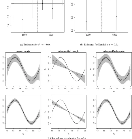
4.1. Results
In this section we focus on the results obtained for the outcome equation, which is the one of
interest, as well as for the Kendall’sτ. Figure 1 displays the findings for case of data generated
according to scenario I. In this case, estimates are shown for the models based on:
• logit and inverse Gaussian margins with a Clayton copula (the outcome distribution is
mis-specified);
• logit and gamma margins with the classic Gaussian copula (the dependence structure is
mis-specified).
We chose the inverse Gaussian since it has the same mean as that of the gamma (Stasinopoulos et al.,
2017b), hence facilitating the comparison of estimates. When the model is correctly specified,
all mean estimates are very close to the true values and, as expected, their variability decreases
as the sample size increases. Misspecifying the marginal outcome distribution has a substantial
detrimental impact on all the parameter estimates, hence stressing the importance of choosing a
suitable outcome distribution in practical situations. Using the incorrect dependence also affects
the estimates (although in a less pronounced manner), hence emphasizing the potential benefits
of allowing for non-Gaussian structures. We also fitted models based on other copulae (such as
Frank, FGM, AMH and Joe available inGJRM) and the findings were similar. Moreover, the
cor-rect model was always selected by criteria such as AIC and BIC. Misspecifying the link function
(using probit and cloglog links) for the selection equation did not significantly affect the results.
Perhaps this is not surprising given that all links produced very similar predicted probabilities for
the selection response variable. Nevertheless, the availability of different link functions allowed
us to assess the impact of this misspecification on the parameters of interest. Using a 2.20-GHz
Intel(R) Core(TM) computer running Windows 7, model fitting took on average 2 seconds for
n = 1000, and 7 seconds forn = 5000. Increasing the number of basis functions to 20 did not
have a noticeable impact on the results but increased computing time by about20%on average.
Moreover, using other spline definitions (such as penalized cubic regression splines and P-splines)
virtually led to identical results. These findings were somewhat expected and have also been
documented in similar contexts by (Wood, 2017).
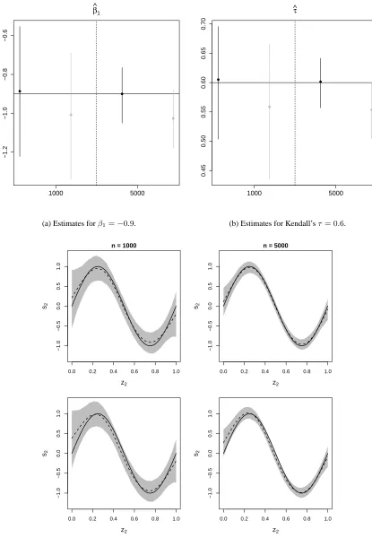
The results for scenario II are given in Figure 2. Estimates are shown for the models based
on:
• probit and Gaussian margins with a Gumbel copula (the correct model);
• probit and Gaussian margins with the classic Gaussian copula (the dependence structure is
misspecified).
The conclusions are similar to those obtained for scenario I. Specifically, for the correctly specified
model the mean estimates are close to the true values and the variability of the estimates decreases
all the parameter estimates. Using various copulae the correct model was always picked by AIC
and BIC, link function misspecification did not really alter the estimates, computing times were
similar to those found for scenario I, and increasing the number of basis functions and using
different spline’s definitions did not have a tangible impact on the results. We have not reported
the results obtained when misspecifying the marginal outcome distribution as these were nearly
identical to those obtained for scenario I.
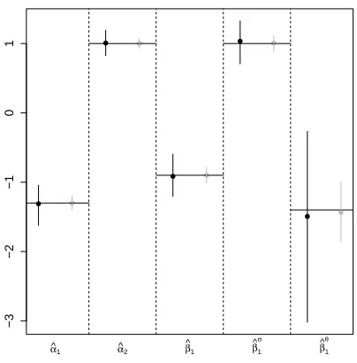
The results for scenario III are given in Figure 3 and are based on probit and Gumbel margins
with a Joe copula (the correct model). This scenario is more complex than the previous ones in
that all distributional parameters are specified as functions of covariates. The findings show that
the approach can estimate all the model components fairly well, and that the estimates improve as
the sample size increases. The components in the additive predictor of the dependence parameter
are estimated less precisely than those of the others. This indicates that the effects of covariates
on the association between the selection and outcome equations may be more difficult to estimate.
This is reasonable given that the likelihood contributions for the association parameter come from
the selected sample of observations only. Average computing times were about 16 seconds for
n = 1000, and 42 seconds forn = 5000. We also tested the models under misspecification of
the dependence structure and marginal outcome distribution. In the former case, the findings were
similar to those for scenarios I and II; using the incorrect copula affects adversely the
parame-ter estimates in parame-terms of bias and efficiency. In the latparame-ter case, the models failed to converge in
many of the iterations (55%forn = 1000and43%forn = 5000) and for the converged models
computing times were between 20 and 30 times those reported above. This highlighted the
impor-tance of choosing an appropriate distribution for the outcome variable, especially when the model
−1.4 −1.2 −1.0 −0.8 −0.6 −0.4
β^1
1000 5000
(a) Estimates forβ1=−0.9.
0.0 0.2 0.4 0.6 τ ^ 1000 5000
(b) Estimates for Kendall’sτ= 0.6.
0.0 0.2 0.4 0.6 0.8 1.0
−1.0 −0.5 0.0 0.5 1.0 correct model z2 s2
0.0 0.2 0.4 0.6 0.8 1.0
−1.0 −0.5 0.0 0.5 1.0 misspecified margin z2 s2
0.0 0.2 0.4 0.6 0.8 1.0
−1.0 −0.5 0.0 0.5 1.0 misspecified copula z2 s2
0.0 0.2 0.4 0.6 0.8 1.0
−1.0 −0.5 0.0 0.5 1.0 z2 s2
0.0 0.2 0.4 0.6 0.8 1.0
−1.0 −0.5 0.0 0.5 1.0 z2 s2
0.0 0.2 0.4 0.6 0.8 1.0
−1.0 −0.5 0.0 0.5 1.0 z2 s2
[image:14.612.69.527.139.622.2](c) Smooth curve estimates fors2(·).
−1.2
−1.0
−0.8
−0.6
β^1
1000 5000
(a) Estimates forβ1=−0.9.
0.45
0.50
0.55
0.60
0.65
0.70
τ ^
1000 5000
(b) Estimates for Kendall’sτ= 0.6.
0.0 0.2 0.4 0.6 0.8 1.0
−1.0
−0.5
0.0
0.5
1.0
n = 1000
z2 s2
0.0 0.2 0.4 0.6 0.8 1.0
−1.0
−0.5
0.0
0.5
1.0
n = 5000
z2 s2
0.0 0.2 0.4 0.6 0.8 1.0
−1.0
−0.5
0.0
0.5
1.0
z2 s2
0.0 0.2 0.4 0.6 0.8 1.0
−1.0
−0.5
0.0
0.5
1.0
z2 s2
[image:15.612.92.507.53.653.2](c) Smooth curve estimates fors2(·).
Figure 2: Scenario II. In Figures (a) and (b), black circles and vertical bars refer to the results obtained under the correct model, and grey circles and bars to those obtained when the dependence structure is misspecified. Circles indicate mean estimates while bars represent the estimates’ ranges resulting from5%and95%quantiles. In Figure (c), mean estimates are represented by dashed lines and point-wise ranges resulting from5%and
−3
−2
−1
0
1
α^1 α^2 β^
1 β ^ 1 σ β ^ 1 θ
(a) Estimates for the parametric components in the model.
0.0 0.2 0.4 0.6 0.8 1.0
−1.0 −0.5 0.0 0.5 z2 s1
0.0 0.2 0.4 0.6 0.8 1.0
−1.0 −0.5 0.0 0.5 1.0 z2 s2
0.0 0.2 0.4 0.6 0.8 1.0
−1.0 −0.5 0.0 0.5 1.0 z2 s3
0.0 0.2 0.4 0.6 0.8 1.0
−1.0 −0.5 0.0 0.5 1.0 z2 s1
0.0 0.2 0.4 0.6 0.8 1.0
−1.0 −0.5 0.0 0.5 1.0 z2 s2
0.0 0.2 0.4 0.6 0.8 1.0
−1.0 −0.5 0.0 0.5 1.0 z2 s3
[image:16.612.203.405.92.297.2](b) Smooth curve estimates fors1(·),s2(·)ands3(·).
5. Empirical application
As a real world application, we consider the study of the effects of insurance status and
man-aged care on hospitalization spells previously analysed by Prieger (2002). The data set is based
on a nationally representative survey of US medical care (Medical Expenditure Panel Survey) and
it contains information about the length of individuals’ hospital stays in 1996 along with factors
such as membership in health maintenance organization, type of insurance, health status,
demo-graphic variables, sex, race, marriage, employment status and quantitative variables including age,
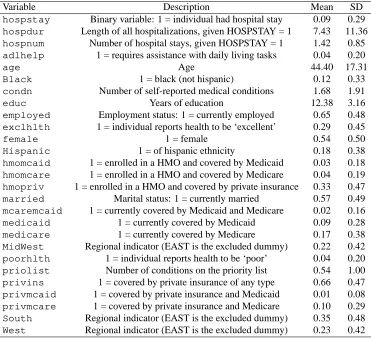
years of education, number of self-reported medical conditions and number of conditions on the
priority list. A detailed description of the variables can be found in Table 3 given in Appendix
B. The sample used in the analysis consists of 14,946 observations. The response variable for
the selection equation is whether an individual had a hospital stay. If the link between hospital
admittance and the spell of hospital stay is not through observables alone then sample selection
bias arises and using a univariate regression approach is not adequate.
These data were studied by Prieger (2002) who motivates the use of the gamma distribution
to model the length of hospital stay, uses a probit selection equation, and fits three models based
on the assumption of independence, and on the Gaussian and FGM copulae. All the covariates
entered the selection and outcome equations parametrically. Prieger found, for instance, that
non-random sample selection was present and, based on various criteria, chose the FGM copula which
produced a negative and significant estimated dependence between the two equations.
We re-analyse these data by considering a wider set of marginal outcome distributions, link
functions and copulae. We also employ smooth functions of age and years of education (using
the same set up described in the simulation study), and specify all parameters of the marginal
distributions as functions of additive predictors.
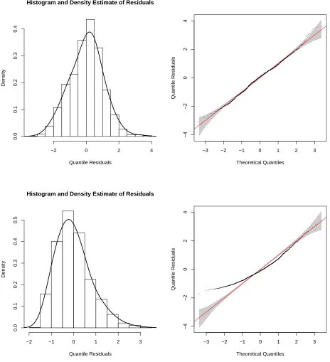
Regarding the marginals, we chose the probit link and found that the inverse Gaussian
in-stead of the gamma distribution provides the best fit as judged by the plots of normalised quantile
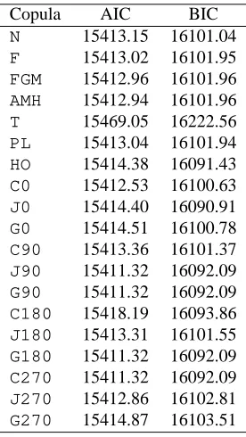
residuals (Stasinopoulos et al., 2017b) and information criteria (see Figure 4). Using the logit and
cloglog links for the selection equation did not affect the results. As for the choice of copula,
we started off with the Gaussian, Frank, FGM, AMH, Student-t and Plackett (since they allow
for both positive and negative dependence) and then employed all of the remaining copulae that
were consistent with the sign of dependence found. For this empirical application, we tried all
copulae available as there was not a clear indication of positive or negative dependence. In all
cases, the values forτ were very close to zero as well as non significantly different from zero for
Histogram and Density Estimate of Residuals
Quantile Residuals
Density
−2 0 2 4
0.0
0.1
0.2
0.3
0.4
−3 −2 −1 0 1 2 3
−4
−2
0
2
4
Theoretical Quantiles
Quantile Residuals
Histogram and Density Estimate of Residuals
Quantile Residuals
Density
−2 −1 0 1 2 3
0.0
0.1
0.2
0.3
0.4
0.5
−3 −2 −1 0 1 2 3
−4
−2
0
2
4
Theoretical Quantiles
[image:18.612.69.533.116.625.2]Quantile Residuals
Copula AIC BIC
N 15413.15 16101.04
F 15413.02 16101.95
FGM 15412.96 16101.96
AMH 15412.94 16101.96
T 15469.05 16222.56
PL 15413.04 16101.94
HO 15414.38 16091.43
C0 15412.53 16100.63
J0 15414.40 16090.91
G0 15414.51 16100.78
C90 15413.36 16101.37
J90 15411.32 16092.09
G90 15411.32 16092.09
C180 15418.19 16093.86
J180 15413.31 16101.55
G180 15411.32 16092.09
C270 15411.32 16092.09
J270 15412.86 16102.81
[image:19.612.233.371.40.285.2]G270 15414.87 16103.51
Table 2: Comparison of AIC and BIC values under different copula assumptions, and probit and inverse Gaussian margins.
copulae were fairly close in most cases (see Table 2). This was somewhat expected given that no
significant association between the equations was detected with all copulae.
Appendix B shows the summary output obtained from the final model which is based on the
270◦ Clayton copula and probit and inverse Gaussian margins. Employing other copulae (for
in-stance,G180,G90,J90) produced nearly identical results. The main findings can be summarised
as follows:
• As argued by Prieger (2002), the association (positive or negative) between admittance and
length of stay may suggest the presence of specific selection mechanisms. He also states
that there is no a priori expectation on the sign of the dependence. As opposed to Prieger’s
finding of a negative association between the selection and outcome equations, we found that
non-random sample selection is not present when using the inverse Gaussian (the
distribu-tion supported by the data). However, when using the gamma as outcome distribudistribu-tion and
the FGM copula (as well as other copulae such as Gaussian, Frank, Student-t and Plackett)
we found that the association parameter is negative and significant (e.g., τˆ = −0.514 with
(−0.589,−0.428)as95%confidence interval forτ), which is line with Prieger’s result. Our
simulations show that misspecifying the outcome distribution can have a severe detrimental
impact on the parameter estimates including the Kendall’sτ. This all suggests that Prieger’s
finding is biased by the choice of gamma distribution for the outcome equation.
observe for instance that the insurance variables privins, medicare and medicaid
increase the probability of hospital admittance, that such effects are either reinforced or
tem-pered by privmcare, privmcaid and mcaremcaid, and that covariates hmopriv,
hmomcare, hmomcaidhave no significant effect on hospital admittance. Moreover,
vari-ables condn, priolist, adlhelp and poorhlth increase the probability of hospital
admittance. These findings are consistent with those of Prieger (2002) to which the reader is
referred to for a more through discussion.
The estimated smooth functions for age and years of education are displayed in Figure 6,
Appendix B. The effect of education is not significant and nearly linear (see also respective
p-value reported in the summary output). On the other hand, the effect of age is non-linear
and significant; its shape suggests that age decreases the probability of hospital admittance
up to about 45 years and then increases such probability afterward. This may be due to the
fact that age embodies productivity and life-cycle effects that are likely to affect the responses
considered in this study non-linearly.
• Outcome equation: from the summary output for equation 2 we observe for example that
poorhlth andadlhelpsignificantly lengthen the stay in hospital, hmopriv decreases
the stay, thatprivins does not influence the outcome, and thatmedicaredecreases the
duration of stay. Our findings are in agreement with those by Prieger (2002). Note, however,
that different distributions and parametrizations are employed in two analyses, hence an exact
comparison is not possible.
The estimated smooth function for years of education (not shown here) is linear and
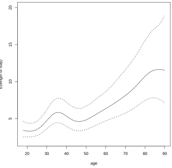
non-significant (as also supported by the respective p-value in the summary output). Figure 5
shows the effect of age on the average hospital stay duration. It suggests that as age increases
the average length of hospital stay increases up to 35, decreases and then increases again
after 45. It may be argued that, given the width of the confidence intervals, a straight line
relationship is also suitable here. In the absence of a formal test of linearity of a smooth
function for the current modelling framework, an informal indication of whether a simpler
model would be appropriate can be obtained using information criteria. Specifically, AIC
and BIC values are15411.32and16092.09for the model with non-linear effect for age, and
15420.02and16064.05for the model with linear effect; the conclusions reached by the two
criteria are discordant and a definitive answer can not be provided in this case.
20 30 40 50 60 70 80 90
5
10
15
20
age
E(length of sta
[image:21.612.127.465.77.409.2]y)
Figure 5: Effect of age on the the mean of hospital stays (black continuous line). The dashed lines represent 95% confidence intervals.
as those for the copula model’s outcome equation. This is not surprising given that, as
dis-cussed previously, no significant association between the selection and outcome equations
was found.
• Copula models where dependence parameter θ3 was specified as a function of various
com-binations of covariates were also fitted. This allowed us to capture potential heterogeneity
in the selection process, hence possibly justifying the overall non significance of the
depen-dence parameter potentially due to compensating effects. However, the results consistently
pointed to the lack of significant association between the selection and outcome equations.
The analysis presented in this section has extended Prieger’s one by considering a wider set
of marginal distributions and copulae as well as non-linear covariate effects. Using the proposed
modeling framework we found evidence of linearity for some covariate effects and that
non-random sample selection does not seem to be present when employing the outcome distribution
selec-tion bias may be regarded as a ‘non-finding’ at first, we argue that our result still has important
implications for the study of selection bias since using a more restrictive set of modelling choices
may lead to unfounded speculations on the presence of certain selection mechanisms.
6. Discussion
We have introduced an extension of GAMLSS which accounts for non-random sample
selec-tion. The proposed approach is flexible in that it allows for different parametric distributions of
the selection and outcome variables, several types of dependence structures between the model’s
equations, and for various types of covariate effects. Using the special case of one-parameter
exponential families, we have elucidated the nature of the correction mechanism underlying the
selection approach. Parameter estimation is carried out within a penalized likelihood framework
based on a trust region algorithm with integrated smoothing parameter selection. The approach
has been illustrated in simulation and through a case study. All new developments have been
incorporated in theRpackageGJRM(Marra and Radice, 2018).
Many marginal distributions and copulae have been considered in this work and we plan on
extending the set of choices available. Future research will look into generalising the proposed
sample selection GAMLSS framework to empirical situations where rules of double selection
exist (e.g., Smith, 2003; Zhang et al., 2015), exploiting for instance C- and D-Vine constructions.
Acknowledgment
We would like to thanks the two anonymous reviewers for their well thought out comments
and suggestions which have helped to improve considerably the quality and massage of the article.
Appendix A:Rcodes to generate data for scenarios I, II and III
For the first two scenarios, data were generated using the followingRcode.
library(copula); library(gamlss.dist)
library(GJRM)
cor.cov <- matrix(0.5, 3, 3); diag(cor.cov) <- 1
s1 <- function(x) x + exp(-30*(x - 0.5)^2) s2 <- function(x) sin(2*pi*x)
cov <- rMVN(1, rep(0,3), cor.cov)
cov <- pnorm(cov)
x1 <- cov[, 1]
x2 <- cov[, 2]
x3 <- round(cov[, 3])
eta_mu1 <- -0.8 - 1.3*x1 + s1(x2) + x3 eta_mu2 <- 0.1 + s2(x2) - 0.9*x3
speclist1 <- list( mu = eta_mu1, sigma = 1)
if(scen == 1){
speclist2 <- list( mu = exp(eta_mu2), sigma = 3)
spec <- mvdc(copula = Cop, c("LO", "GA"), list(speclist1, speclist2) )
Cop <- archmCopula(family = "clayton", dim = 2, param = 3)
}else{
speclist2 <- list( mu = eta_mu2, sigma = 2)
spec <- mvdc(copula = Cop, c("NO", "NO"), list(speclist1, speclist2) )
Cop <- archmCopula(family = "gumbel", dim = 2, param = 2.5)
}
resp <- rMvdc(1, spec)
resp[1] <- resp[1] > 0
c(resp, x1, x2, x3)
}
Packagecopula(Yan, 2007) contains functionsarchmCopula(),mvdc()andrMvdc()
which allow one to simulate from the desired copula. Packagegamlss.dist(Stasinopoulos et al.,
2017a) contains all the functions required to simulate the marginals adopted here, andrMVN()
(fromGJRM) allows one to simulate Gaussian correlated variables. The correlation matrix used to
associate the three simulated Gaussian covariates iscor.cov, whereascov <- pnorm(cov)
allows one to obtain Uniform(0,1) correlated covariates (e.g., Gentle, 2003). A balanced binary
regressor is created usinground(cov[, 3]). Functionss1ands2produce curves with
these are transformed inspeclist1and speclist2(and also archmCopulafor scenario
III below) to ensure that the restrictions on the parameters’ spaces of the bivariate distributions are
maintained. In the first two scenarios the copula dependence parameters are set to 3 and 2.5 which
correspond to a Kendall’sτ of0.6.
The code used to generate data for scenario III is given below.
datagen3 <- function(cor.cov, s1, s2, s3){
cov <- rMVN(1, rep(0,3), cor.cov) cov <- pnorm(cov)
z1 <- cov[, 1]
z2 <- cov[, 2]
z3 <- round(cov[, 3])
eta_mu1 <- -.8 - 1.3*z1 + s1(z2) + z3
eta_mu2 <- 0.1 + s2(z2) - 0.9*z3
eta_si2 <- 0.5 + z3
eta_the <- 1.1 - 1.4*z1 + s3(z2)
Cop <- archmCopula(family = "joe", dim = 2,
param = exp(eta_the) + 1 + 1e-07)
speclist1 <- list( mu = eta_mu1, sigma = 1)
speclist2 <- list( mu = eta_mu2, sigma = sqrt(exp(eta_si2)))
spec <- mvdc(copula = Cop, c("NO", "GU"), list(speclist1, speclist2) )
resp <- rMvdc(1, spec)
resp[1] <- resp[1] > 0
c(resp, z1, z2, z3)
Variable Description Mean SD
hospstay Binary variable: 1 = individual had hospital stay 0.09 0.29
hospdur Length of all hospitalizations, given HOSPSTAY = 1 7.43 11.36
hospnum Number of hospital stays, given HOSPSTAY = 1 1.42 0.85
adlhelp 1 = requires assistance with daily living tasks 0.04 0.20
age Age 44.40 17.31
Black 1 = black (not hispanic) 0.12 0.33
condn Number of self-reported medical conditions 1.68 1.91
educ Years of education 12.38 3.16
employed Employment status: 1 = currently employed 0.65 0.48
exclhlth 1 = individual reports health to be ‘excellent’ 0.29 0.45
female 1 = female 0.54 0.50
Hispanic 1 = of hispanic ethnicity 0.18 0.38
hmomcaid 1 = enrolled in a HMO and covered by Medicaid 0.03 0.18
hmomcare 1 = enrolled in a HMO and covered by Medicare 0.04 0.19
hmopriv 1 = enrolled in a HMO and covered by private insurance 0.33 0.47
married Marital status: 1 = currently married 0.57 0.49
mcaremcaid 1 = currently covered by Medicaid and Medicare 0.02 0.16
medicaid 1 = currently covered by Medicaid 0.09 0.28
medicare 1 = currently covered by Medicare 0.17 0.38
MidWest Regional indicator (EAST is the excluded dummy) 0.22 0.42
poorhlth 1 = individual reports health to be ‘poor’ 0.04 0.20
priolist Number of conditions on the priority list 0.54 1.00
privins 1 = covered by private insurance of any type 0.66 0.47
privmcaid 1 = covered by private insurance and Medicaid 0.01 0.08
privmcare 1 = covered by private insurance and Medicare 0.10 0.29
South Regional indicator (EAST is the excluded dummy) 0.35 0.48
[image:26.612.117.488.41.381.2]West Regional indicator (EAST is the excluded dummy) 0.23 0.42
Table 3: MEPS data: variable definitions and summary statistics. All hospitalization variables are for 1996. This table is from Prieger (2002).
Appendix B: summary results from model selected in empirical application
COPULA: 270 Clayton
MARGIN 1: Bernoulli
MARGIN 2: inverse Gaussian
EQUATION 1
Link function for mu.1: probit
Formula: y1 ~ privins + medicare + medicaid + hmopriv + hmomcare + hmomcaid +
privmcare + privmcaid + mcaremcaid + condn + priolist + exclhlth +
poorhlth + adlhelp + MidWest + South + West + female + s(age) +
Black + Hispanic + s(educ) + married + employed
Parametric coefficients:
Estimate Std. Error z value Pr(>|z|)
(Intercept) -1.850351 0.069180 -26.747 < 2e-16 ***
privins 0.188455 0.054576 3.453 0.000554 ***
medicare 0.301470 0.092851 3.247 0.001167 **
hmopriv 0.030331 0.042296 0.717 0.473299
hmomcare 0.026591 0.076898 0.346 0.729490
hmomcaid -0.037339 0.092341 -0.404 0.685947
privmcare -0.208284 0.080720 -2.580 0.009870 **
privmcaid 0.355882 0.157468 2.260 0.023820 *
mcaremcaid -0.493067 0.111832 -4.409 1.04e-05 ***
condn 0.082802 0.010335 8.012 1.13e-15 ***
priolist 0.065037 0.019043 3.415 0.000637 ***
exclhlth -0.149980 0.039539 -3.793 0.000149 ***
poorhlth 0.219394 0.064518 3.400 0.000673 ***
adlhelp 0.338518 0.064002 5.289 1.23e-07 ***
MidWest 0.020925 0.047101 0.444 0.656850
South 0.009535 0.043418 0.220 0.826183
West -0.085877 0.048660 -1.765 0.077589 .
female 0.149305 0.032633 4.575 4.76e-06 ***
Black -0.028681 0.049880 -0.575 0.565286
Hispanic 0.084497 0.046239 1.827 0.067643 .
married 0.105973 0.034991 3.029 0.002457 **
employed -0.163872 0.040729 -4.023 5.74e-05 ***
---Signif. codes: 0 ‘***’ 0.001 ‘**’ 0.01 ‘*’ 0.05 ‘.’ 0.1 ‘ ’ 1
Smooth components’ approximate significance:
edf Ref.df Chi.sq p-value
s(age) 6.008 7.176 37.165 5.33e-06 ***
s(educ) 1.785 2.236 1.369 0.496
---Signif. codes: 0 ‘***’ 0.001 ‘**’ 0.01 ‘*’ 0.05 ‘.’ 0.1 ‘ ’ 1
EQUATION 2
Link function for mu.2: log
Formula: y2 ~ privins + medicare + medicaid + hmopriv + hmomcare + hmomcaid +
privmcare + privmcaid + mcaremcaid + condn + priolist + exclhlth +
poorhlth + adlhelp + MidWest + South + West + female + s(age) +
Black + Hispanic + s(educ) + married + employed
Parametric coefficients:
Estimate Std. Error z value Pr(>|z|)
(Intercept) 2.244987 0.169074 13.278 < 2e-16 ***
privins 0.167173 0.129127 1.295 0.195444
medicaid -0.015643 0.156081 -0.100 0.920165
hmopriv -0.443685 0.106618 -4.161 3.16e-05 ***
hmomcare 0.523395 0.216804 2.414 0.015772 *
hmomcaid -0.080578 0.186132 -0.433 0.665082
privmcare -0.096168 0.177819 -0.541 0.588631
privmcaid 0.509183 0.242352 2.101 0.035640 *
mcaremcaid 0.143036 0.220478 0.649 0.516496
condn 0.004007 0.022184 0.181 0.856672
priolist 0.082884 0.043742 1.895 0.058118 .
exclhlth -0.047858 0.089880 -0.532 0.594402
poorhlth 0.434519 0.143721 3.023 0.002500 **
adlhelp 0.355209 0.145970 2.433 0.014956 *
MidWest -0.188903 0.111958 -1.687 0.091552 .
South -0.096852 0.105099 -0.922 0.356777
West -0.383978 0.112817 -3.404 0.000665 ***
female -0.484550 0.092887 -5.217 1.82e-07 ***
Black 0.366785 0.114616 3.200 0.001374 **
Hispanic 0.067553 0.093491 0.723 0.469948
married -0.123221 0.078603 -1.568 0.116966
employed -0.113859 0.081580 -1.396 0.162810
---Signif. codes: 0 ‘***’ 0.001 ‘**’ 0.01 ‘*’ 0.05 ‘.’ 0.1 ‘ ’ 1
Smooth components’ approximate significance:
edf Ref.df Chi.sq p-value
s(age) 6.791 7.908 52.609 1.16e-08 ***
s(educ) 1.000 1.000 0.007 0.934
---Signif. codes: 0 ‘***’ 0.001 ‘**’ 0.01 ‘*’ 0.05 ‘.’ 0.1 ‘ ’ 1
EQUATION 3
Link function for sigma2: log
Formula: ~privins + medicare + medicaid + hmopriv + hmomcare + hmomcaid +
privmcare + privmcaid + mcaremcaid + condn + priolist + exclhlth +
poorhlth + adlhelp + MidWest + South + West + female + s(age) +
Black + Hispanic + s(educ) + married + employed
Parametric coefficients:
Estimate Std. Error z value Pr(>|z|)
(Intercept) -1.437645 0.198799 -7.232 4.77e-13 ***
medicare 0.004227 0.207456 0.020 0.98375
medicaid 0.365449 0.207283 1.763 0.07789 .
hmopriv -0.270515 0.118284 -2.287 0.02220 *
hmomcare 0.505104 0.190237 2.655 0.00793 **
hmomcaid 0.218626 0.215001 1.017 0.30922
privmcare 0.049511 0.198518 0.249 0.80305
privmcaid -0.845025 0.326819 -2.586 0.00972 **
mcaremcaid -0.460742 0.261357 -1.763 0.07792 .
condn 0.032792 0.022851 1.435 0.15128
priolist -0.072283 0.039988 -1.808 0.07067 .
exclhlth 0.047090 0.116003 0.406 0.68479
poorhlth -0.088651 0.143464 -0.618 0.53662
adlhelp -0.223425 0.132612 -1.685 0.09203 .
MidWest -0.159945 0.124918 -1.280 0.20040
South -0.167665 0.114324 -1.467 0.14249
West -0.039339 0.127541 -0.308 0.75774
female -0.100680 0.092344 -1.090 0.27559
Black -0.235727 0.134401 -1.754 0.07945 .
Hispanic 0.018131 0.124514 0.146 0.88423
married -0.045687 0.092462 -0.494 0.62123
employed 0.136274 0.109383 1.246 0.21282
---Signif. codes: 0 ‘***’ 0.001 ‘**’ 0.01 ‘*’ 0.05 ‘.’ 0.1 ‘ ’ 1
Smooth components’ approximate significance:
edf Ref.df Chi.sq p-value
s(age) 2.255 2.868 4.803 0.156
s(educ) 1.000 1.000 0.322 0.570
EQUATION 4
Link function for theta: log(- .)
Formula: ~1
Parametric coefficients:
Estimate Std. Error z value Pr(>|z|)
(Intercept) -20.68 348.64 -0.059 0.953
n = 14946 n.sel = 1346
sigma2 = 0.293(0.207,0.42)
total edf = 87.8
20 30 40 50 60 70 80 90
−0.2
0.0
0.2
0.4
0.6
age
s(age
,6.01)
0 5 10 15
−0.2
−0.1
0.0
0.1
educ
s(educ
[image:30.612.92.504.99.302.2],1.79)
Figure 6: Selection equation: smooth effects for age and years of education and associated95%point-wise intervals obtained from the final model which is based on the270◦Clayton copula and probit and inverse Gaussian margins. The rug plot, at the bottom of each graph, shows the covariate
values. The number in brackets in the y-axis of each plot’s caption represents the effective degrees of freedom of the respective smooth curve.
Andrews, D.W.K., Schafgans, M.M.A., 1998. Semiparametric estimation of the intercept of a sample selection model. Review of Economic Studies 65, 497–517.
Chen, S., Zhou, Y., 2010. Semiparametric and nonparametric estimation of sample selection models under symmetry. Journal of Econometrics 157, 143–150.
Chib, S., Greenberg, E., Jeliazkov, I., 2009. Estimation of semiparametric models in the presence of endogeneity and sample selection. Journal of Computational and Graphical Statistic 18, 321–348.
Collier, D., Mahoney, J., 1996. Insights and pitfalls: selection bias in qualitative research. World Politics 49, 56–91.
Das, M., Newey, W., Vella, F., 2003. Nonparametric estimation of sample selection models. Review of Economic Studies 70, 33–58.
Ding, P., 2014. Bayesian robust inference of sample selection using selection-models. Journal of Multivariate Analysis 124, 451–464.
Eilers, P., Marx, B., 1996. Flexible smoothing withB-splines and penalties. Statistical Science 11, 89–121.
Gallant, R.A., Nychka, D.W., 1987. Semi-nonparametric maximum likelihood estimation. Econometrica 55, 363–390.
Genius, M., Strazzera, E., 2008. Applying the copula approach to sample selection modelling. Applied Economics 40, 1443–1455.
Gentle, J.E., 2003. Random number generation and Monte Carlo methods. Springer-Verlag, London.
Gronau, R., 1974. Wage comparisons: A selectivity bias. Journal of Political Economy 82, 1119–1143.
Heckman, J., 1976. The common structure of statistical models of truncation, sample selection and limited dependent variables and a simple estimator for such models. Annals of Economic and Social Measurement 5, 475–492.
Heckman, J., 1979. Sample selection bias as a specification error. Econometrica 47, 153–162.
Lee, D.S., 2008. Training, wages, and sample selection: Estimating sharp bounds on treatment effects. Review of Economic Studies 76, 1071–1102.
Lennox, C., Francis, J., Wang, Z., 2012. Selection models in accounting research. The Accounting Review 87, 589–616.
Lewis, H.G., 1974. Comments on selectivity biases in wage comparisons. Journal of Political Economy 82, 1145–1155.
Marchenko, J.V., Genton, M.G., 2012. A Heckman selection-t model. Journal of the American Statistical Association 107, 304– 317.
Marra, G., Radice, R., 2013a. Estimation of a regression spline sample selection model. Computational Statistics and Data Analysis 61, 158–173.
Marra, G., Radice, R., 2013b. A penalized likelihood estimation approach to semiparametric sample selection binary response modeling. Electronic Journal of Statistics 7, 1432–1455.
Marra, G., Radice, R., 2018. GJRM: Generalised Joint Regression Modelling. URL: http://CRAN.R-project.org/package=GJRM. r package version 0.2.
Marra, G., Radice, R., Bärnighausen, T., Wood, S.N., McGovern, M.E., 2017. A simultaneous equation approach to estimating HIV prevalence with nonignorable missing responses. Journal of the American Statistical Association 112(518), 484–496.
Marra, G., Wyszynski, K., 2016. Semi-parametric copula sample selection models for count responses. Computational Statistics & Data Analysis 104, 110–129.
Nelsen, R., 2006. An Introduction to Copulas. second ed., Springer-Verlag, New York.
Newey, W.K., 2009. Two-step series estimation of sample selection models. Econometrics Journal 12, S217–S229.
Powell, J.L., 1994. Estimation of semiparametric models, in: Heckman, J.J., Leamer, E. (Eds.), Handbook of econometrics. Elsevier, Amsterdam, pp. 5307–5368.
Prieger, J.E., 2002. A flexible parametric selection model for non-normal data with application to health care usage. Journal of Applied Econometrics 17, 367–392.
Radice, R., Marra, G., Wojtys, M., 2016. Copula regression spline models for binary outcomes. Statistics and Computing 26, 981–995.
Rigby, R.A., Stasinopoulos, D.M., 2005. Generalized additive models for location, scale and shape. Applied Statistics 54, 507–554.
Ruppert, D., Wand, M., Carroll, R., 2003. Semiparametric Regression. Cambridge University Press, New York.
Schweizer, B., 1991. Thirty years of copulas., in: Dall’Aglio, G., Kotz, S., Salinetti, G. (Eds.), Advances in Probability Distribu-tions with Given Marginals: Beyond the Copulas. Dordrecht: Kluwer. chapter 2, pp. 13–50.
Sklar, A., 1959. Fonctions de répartition à n dimensions et leurs marges. Publications de l’Institut de Statistique de L’Université de Paris 8, 229–231.
Smith, M.D., 2003. Modelling sample selection using Archimedean copulas. Econometrics Journal 6, 99–123.
Stasinopoulos, M., Rigby, R., Akantziliotou, C., Voudouris, V., Heller, G., Ospina, R., Motpan, N., McElduff, F., Djennad, M., Enea, M., Ghalanos, A., Argyropoulos, C., 2017a. gamlss.dist: Distributions for Generalized Additive Models for Location Scale and Shape. URL:http://CRAN.R-project.org/package=gamlss.dist. r package version 5.0-3.
Stasinopoulos, M., Rigby, R., Heller, G., Voudouris, V., Bastiani, F.D., 2017b. Flexible Regression and Smoothing: Using GAMLSS in R. Chapman & Hall/CRC, London.
van der Vaart, A.W., 2000. Asymptotic Statistics. Cambridge University Press.
Vella, F., 1998. Estimating models with sample selection bias: A survey. Journal of Human Resources 33, 127–169.
Wiesenfarth, M., Kneib, T., 2010. Estimating the relationship of women’s education and fertility in Botswana using an instrumental variable approach to semiparametric expectile regression. Journal of the Royal Statistical Society Series C 59, 381–404.
Wojty´s, M., Marra, G., Radice, R., 2016. Copula regression spline sample selection models: theRpackageSemiParSampleSel. Journal of Statistical Software 71(6), 1–66.
Wood, S.N., 2017. Generalized Additive Models: An Introduction With R, Second Edition. Chapman & Hall/CRC, London.
Wyszynski, K., Marra, G., 2017. Sample selection models for count data in R. Computational Statistics , 1–28.
Yan, J., 2007. Enjoy the joy of copulas: With a package copula. Journal of Statistical Software 21, 1–21.
Zhang, R., Inder, B.A., Zhang, X., 2015. Bayesian estimation of a discrete response model with double rules of sample selection. Computational Statistics and Data Analysis 86, 81–96.