http://dx.doi.org/10.4236/apm.2016.63010
A Global Reduction Based Algorithm for
Computing Homology of Chain Complexes
Madjid Allili, David Corriveau
Department of Mathematics, Bishop’s University, Sherbrooke, Canada
Received 22 September 2015; accepted 21 February 2016; published 26 February 2016
Copyright © 2016 by authors and Scientific Research Publishing Inc.
This work is licensed under the Creative Commons Attribution International License (CC BY). http://creativecommons.org/licenses/by/4.0/
Abstract
In this paper, we propose a new algorithm to compute the homology of a finitely generated chain complex. Our method is based on grouping several reductions into structures that can be encoded as directed acyclic graphs. The organized reduction pairs lead to sequences of projection maps that reduce the number of generators while preserving the homology groups of the original chain complex. This sequencing of reduction pairs allows updating the boundary information in a single step for a whole set of reductions, which shows impressive gains in computational performance compared to existing methods. In addition, our method gives the homology generators for a small additional cost.
Keywords
Homology Algorithm, Chain Complex, Homology Generators
1. Introduction
boundary matrices which are in general sparse [5][6].
Unfortunately, this approach has a very poor running-time and its direct implementation yields exponential bounds. Polynomial time algorithms for computing the SNF were given by Kannan & Bachem [7] and later im-proved by Chou & Collins [8] and Illiopoulos [9]. The best currently known Smith Normal Form algorithms have super cubical complexity [10]. Another generic approach is the method of reduction proposed in [5][11]. In this method the original complex is simplified through a sequence of reductions of cells that preserve the ho-mology groups at each step. The idea is to replace the chain complex (or even the object under study) by a smaller one with the same homology. A reduction consists of cancelling a cell B through an element of its boundary a (reduction pair
(
a B,)
). The two cells are suppressed from the structure of the complex and the boundary homomorphisms are updated. Direct implementations of the reduction method use unordered lists to encode the boundary homomorphisms and have cubical complexity.Several algorithms based on the idea of reduction and that improve the time complexity for particular types of data sets have been designed. For cubical sets embedded in 3, Mrozek et al. proposed a method [12] based on the computation of acyclic subspaces by using lookup tables. Experimentally, this method performed in linear time. Another method running in quasi linear time for finite simplicial complexes embedded in 3 was pro-posed by Delfinado and Edelsbrunner in [13]. For problems dealing with higher dimensions, Mrozek and Batko developed an algorithm [14] based on the concept of coreduction which showed interesting performance results on cubical sets.
Despite the existence of efficient homology algorithms for cubical sets and lower dimension spaces, there re-main many problems where the data is higher dimensional and not cubical. Generally, for these problems it is often difficult to adapt the data because the cost is too high or too complex. In this case, one has to use one of the classical methods: SNF or reduction. However, the classical methods spend most of their time in updating the boundary homomorphisms after each reduction step. This requires repetitive manipulations of the data structures that store the chain complex which incurs a high running time to accomplish the reduction.
An idea is to identify admissible reduction pairs and organize them in a structure that allows efficiently up-dating the boundary information in a single step for a whole set of reductions. This reduces to the minimum ma-nipulations of the data structures that store the boundary information. Our method works as follows. Starting at an arbitrary cell A with a face a in its boundary, we identify successive adjacent admissible pairs of reduction and build the longest possible sequence originating at A. Several sequences can originate at the same cell, and each sequence can be seen as a path in a directed acyclic graph, called a reduction DAG, where nodes are reduc-tion pairs and oriented edges denote an adjacency relareduc-tion between the reducreduc-tion pairs. Given a reducreduc-tion DAG across a chain complex, we achieve a global simplification of the complex by performing all the reductions in the DAG at once. We will establish direct algebraic formulas that allow updating the boundary of remaining cells. The net advantage of our approach is that the boundaries are not explicitly updated after each reduction step. Instead, this information is always preserved implicitly within the data structures and processed globally for each reduction DAG allowing reducing considerably the computational time. The communication [15] con-tains a summary of the method developed systematically here and the preliminary experimentations that are now developed in Section 5.
2. Chain Complexes and Homology
Chain complexes are an algebraic tool for defining and computing homology. Although they are usually defined from geometrical structures such as simplicial or cellular complexes, they can also be considered in an abstract manner as pure algebraic entities. A finitely generated free chain complex
(
,∂)
with coefficients in a ring is a sequence of finitely generated free abelian groups{ }
qq
C ∈ together with a sequence of homomorphisms, called boundary maps or operators,
{
∂q:Cq →Cq−1}
q∈ satisfying ∂q−1∂ =q 0 for all q∈. Typically,0
q
C = for q<0. For each p, the elements of Cp are called p-chains and the kernel of ∂p:Cp →Cp−1 is called the group of p-cycles and denoted Zp =
{
c∈Cp ∂ =pc 0}
. The image of ∂p+1, called the group ofboundaries, is denoted by Bp = ∈
{
c Cp ∃ ∈b Cp+1such that∂p+1b=c}
. Bp is a subgroup of Zp because ofthe property ∂p−1∂ =p 0. The quotient groups Hp:=Zp Bp are the homology groups of the chain complex
Computation of Homology by Reduction of Chain Complexes
The reduction of a chain complex is a procedure that consists of removing successively pairs of generators from the bases of its chain groups while preserving the homology of the original complex. This method is originally motivated by a simple geometric idea known as the collapsing. At the algebraic level, each removal of a pair of generators that form a reduction pair is equivalent to a collection of projection maps
{
πd:Cd→Cd}
d thatsend each generator of the removed pair into 0. Moreover, it projects the other cells into the remaining genera-tors taking into account the modifications of their boundaries caused by the removal of the pair. Let Cd′ =πd
( )
Cdfor each d. It is shown in [5] that C′ is a chain complex and H*
( )
C′ ≅H*( )
C , that is, the homologies of C′and C coincide. To calculate the homology of the original chain complex C, the idea is to define a sequence of projections associated to the removal of pairs in all dimensions and then compute the homology of the resulting chain complex that is the image of the successive projections. A sequence of projections is complete if no other projection can be added to the sequence. Such a sequence always exits when the chain complex is finitely gen-erated. Let
(
C,∂)
be the original chain complex and(
Cf,∂f)
is the final chain complex obtained after acomplete sequence of projections. We already know that the two complexes have the same homology, moreover it is easily observed that if ∂ =f 0 then H*
( )
C ≅H*( )
Cf ≅Cf, that is, the Betti numberd
β is given by the number of d-cells remaining in the complex Cf .
Formally, a reduction pair and its associated collection of projection maps are defined as follows.
Definition 1. Let =
{
Cd,∂d}
be an abstract chain complex. A pair of generators(
a B such that ,)
1,
m m
a∈C − B∈C and ∂B a, = ±1 is called a reduction pair. It induces a collection of group homomorphisms
,
if 1,
,
,
: if ,
,
otherwise,
d
c a
c B d m
B a
c a
c c B d m
B a
c
π
− ∂ = −
∂
∂
= − ∂ =
where c∈Cd and ⋅ ⋅, is the canonical bilinear form on chains.
A way to understand the global reduction of a complex is to reformulate it as an algorithm and follow an ex-ample of its execution. The following implementation is basic and simply aims at understanding the process. For instance, if the chain complex has torsion or if the dimensions are reduced in arbitrary order, then we should re-fer to the more general version of the reduction method described in [5][11]. Also, we use the data structures as defined in section 4.0.
Algorithm 2. Reduction (Complex K) reduces K into K′ using the one-step reduction formula. Consecutive calls of this function will simplify K until it remains unchanged. Finally, if all the boundaries are null, then the homology generators are given by the remaining cells. If not, then we continue the computation of homology by using a classical method such as Smith Normal Form.
1) (Find a reduction pair)
(
a B,)
is a reduction pair if a is a face of B with an incidence coefficient of ±1. If no reduction pair is found, return K unmodified. Otherwise continue. It is assumed that reduction pairs are chosen by decreasing order of dimension. First the highest dimension is reduced, then the lower dimensions.2) (Projection of K) Assign ∂ ←B B. boundary, cob a←a. coboundary and λ← ∂B a, , the coeffi- cient of a in ∂B.
(a) (Update cofaces of a) For all cofaces C of a, add γ B
λ
− ∂ to C. boundary, where γ is ∂C a, , the
coefficient of a in C. boundary.
(b) (Update faces of B) For all faces c of B, add γ cob a
λ
− to c. coboundary, where γ is ∂B c, , the
coefficient of c in B. boundary.
(c) (Project a and B) Remove cells a and B from K. 3) (Return the result) Return the simplified K.
Figure 1.Result of the projection of a complex after one reduction.
given complex, the boundaries of the cells in K are
A a b c d
∂ = + − −
B b e f g
∂ = − + + −
.
C b h i j
∂ = + − −
The pair
(
b C,)
is a reduction pair since the incidence number ∂C b, =1. It follows that2
, 1
, 1
A b
A A A C A C A C
C b
π ∂
′ = = − = − = −
∂
2
, 1
, 1
B b
B B B C B C B C
C b
π ∂ −
′ = = − = − = +
∂
2
, 1
0.
, 1
C b
C C C C C C
C b
π ∂
′ = = − = − =
∂
Clearly, π0 is the identity map since there is no 0-cell removed from the complex and π α α1 = for all α except for π =1b 0. The altered boundaries in the resulting complex K′ are
(
)
A′ A C a c d h i j
∂ = ∂ − = − − − + +
(
)
.B′ B C e f g h i j
∂ = ∂ + = + − + − −
To calculate the homology of the complex we continue the simplifications until ∂ =0 for all dimensions.
3. Computation of Homology by Grouping Reductions
The reduction algorithm chooses reduction pairs in arbitrary order and spends most of its time updating the boundaries at each reduction step. Instead of performing the reductions in arbitrary order, we organize them into reduction sequences that make up reduction directed acyclic graphs (RDAGs). We will show that this is very advantageous algorithmically.
3.1. Forming RDAGs
Starting from an arbitrary cell, we form the maximal possible directed acyclic graph (DAG) whose nodes are reduction pairs and a directed edge between two pairs
(
a B,)
and(
c D,)
means that(
a B,)
is adjacent to(
c D,)
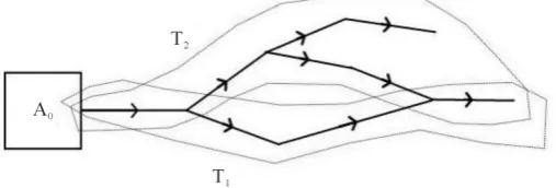
(see definition 4). A directed path in the DAG corresponds to a reduction sequence. That type of reduc-tion sequence affects only adjacent cells to the path and leaves other cells unchanged. Informareduc-tion about each reduction is carried out by the reduced cells. After performing the whole set of reductions, we obtain the reduced complex by extracting the boundary information from the data structures associated to the cells visited by the reduction DAGs.We introduce the main concepts through an example. The example details how the projections of cells are calculated given a reduction sequence. This will show what information is exactly needed to be kept about the original complex in order to be able to rebuild the reduced complex.
Example 3. Consider the complex given inFigure 2. The boundaries of the 2-cell are
A a b h
Figure 2. Example of collapsing by using RDAGs.
B b c f
∂ = − + +
C c d i
∂ = − +
D d e g
∂ = − + +
.
E i j k
∂ = − +
The depicted sequence of reduction pairs originating at cell A is
(
b B,) (
, c C,)
and(
d D,)
. The projection maps at the level of the 2-cell give the following(
)
2, , :
,
b b
b B B
B b
α π α α= − ∂
∂
(
)
2, , :
,
c c
c C C
C c
α π α α= − ∂
∂
(
)
2, , :
,
d d
d D D
D d
α π α α= − ∂
∂
It follows that the projection map associated to the whole sequence is π2=π2dπ π2c 2b. The 2-cell A is the
only cell adjacent to the sequence while the 2-cell E is not adjacent. Their respective projections with respect to the sequence are
(
)
(
)
(
)
(
)
(
)
(
)
(
)
(
)
2 2 2 2 2
2 2 2 2 , , , , , , , , , ,
d c d c
b b d b b d b b d b d
b b c
b b c
b b c
b
b b c
A b
A A A B A B
B b
A B c
A B C
C c
A B c
A B C
C c
B c
A B C
C c
A B C
A B C d D
A B C
D d
A B C
π π π π π λ
λ π λ λ π λ λ π λ
π λ λ λ
λ λ λ λ λ λ
λ
λ λ λ
∂ ′ = = − ∂ = − ∂ − = − − ∂ ∂ − ∂ = − − ∂ − ∂ = − − ∂ = − + ∂ − + = − + − = − + − , , . c
b b c b c d
C d D D d
A B C D
λ
λ λ λ λ λ λ ∂
(
)
2 2 2
2 2
, ,
0 .
d c
d c
E b
E E E B
B b
E B E
π π π
π π
∂
′
= = −
∂
= − ⋅ = =
Each coefficient in the projection is called the coefficient of contribution of the corresponding cell to the pro-jection of A. For instance, −λ λ λb c d is the coefficient of contribution of D in the projection of A. We can compute the coefficients λ λb, c and λd and express concretely the projection of A:
, 1
1
, 1
b
A b B b
λ = ∂ = = −
∂ −
, 1
1
, 1
c
B c C c
λ = ∂ = =
∂
, 1
1
, 1
d
C d D d
λ = ∂ =− =
∂ −
A′ = + − +A B C D
Once a reduction DAG is built, we are interested in building the reduced complex. The cells of the new com-plex are the projected cells of the original comcom-plex. The projection can be used effectively to update or build the boundary operator for each projected cell. In the previous example, the boundary of A′ can be reconstructed from the formula of its projection
.
A′ A B C D f g e a i h
∂ = ∂ + ∂ − ∂ + ∂ = + + − − −
The incidence number of a given cell, say g, with respect to the boundary of the projection of A is computed by adding all the contribution coefficients of the cofaces of g present in the projection of A, each multiplied by the incidence number of g with respect to that coface. A particular coface of g can be present several times in the projection of A if it belongs to different sequences that originate at A.
For instance ∂A g′, is given by
(
)
, b b c b c d , b c d ,
A g′ A λ B λ λC λ λ λ D g λ λ λ D g
∂ = ∂ − + − = − ∂
since D is the only coface of g in the original complex and it is present in the projection of A. Note that the value of ∂D g, is known from the original complex.
[image:6.595.174.455.543.706.2]Thus to calculate the reduced complex, it is enough to keep track of the coefficients of contribution of every reduced cell in any of the projected cells for which it contributes. In general, after a sequence of reductions is achieved, a projected cell adjacent to reduction DAGs will look as depicted in Figure 3.
3.2. Projection Formulas for Grouped Reductions
We define how to organize the reductions and the complex using reduction DAGs.
Definition 4. A cell A1 isadjacent to the pair
(
a A2, 2)
if the cells A1 and A2 are of the same dimension m and a2 is a cell with dimension m−1 in the boundaries of both A1 and A2. A pair(
a A1, 1)
is adjacent to a pair(
a A2, 2)
if A1 is adjacent to(
a A2, 2)
.Definition 5. A reduction DAG is a directed acyclic graph whose nodes are reduction pairs and a directed edge between two pairs
(
a A1, 1)
and(
a A2, 2)
means that(
a A1, 1)
is adjacent to(
a A2, 2)
.Definition 6. A path P from
(
a A to 1, 1)
(
a An, n)
in a reduction DAG G is a reduction sequence(
a A1, 1)
,,(
a An, n)
whose elements are nodes in G and(
a A is adjacent to i, i)
(
ai+1,Ai+1)
, for i=1,,n−1.A cell A is said to be adjacent to a reduction sequence if it is adjacent to some pair of the sequence.
Definition 7. A path from
(
a A1, 1)
to(
a An, n)
in a reduction DAG G is said to originate at A0 if A0 is adjacent to(
a A1, 1)
.Definition 8. A cell not appearing in any reduction DAG is called a projected cell. The cells that appear in a reduction DAG are called reduced cells.
All individual paths originating at a given cell contribute to the projection of the cell. In the following theo-rem, we give a formula to calculate the projection of a cell by considering the contribution of a single path and ignoring the input from other paths and sub-paths. This formula is called “path projection”.
Theorem 9. Let P:
(
a A1, 1)
,,(
a An, n)
be a path originating at A0. The path projection of A0 by the path P is given by( )
0 01
,
n
P i i
i
A A A
π
= = + Γ
∑
where
( )
1 1 i i i j j λ =
Γ = −
∏
, and 1, , j j j j j A a A aλ ∂ −
=
∂ for 1≤i j, ≤n. Γi is called the coefficient of contribution of
i
A in the path projection of A0.
Proof: We proceed by induction on the length of the path. For n=0 or n=1, the path projection formula is easily checked as shown in Example 3. Suppose that the path projection of A0 by the path of length n,
(
1 1)
(
)
: , , , ,
n n n
P a A a A is
( )
0 01
.
n
n
P i i
i
A A A
π
= = + Γ
∑
Adding a
(
n+1)
th pair of reduction(
an+1,An+1)
to the path Pn so that an+1 is a face of An leads to thepath of length
(
n+1)
, Pn+1:(
a A1, 1)
,,(
an+1,An+1)
. The projection of A0 by Pn+1 is equivalent to the pro-jection of
( )
0 nP A
π by the path P1:
(
an+1,An+1)
consisting of a single reduction pair, that is:( )
(
( )
)
( )
( )
( )
1 1 1 1 0 0 0 1 0 1 0 1 1 1 1 0 1 1 , , , . , n n n n nP P P
n
P i i
i
P n
P n
n n
n n
P n n
n n A A A A A a A A A a A a A A A a
π π π
π π π π + = + + + + + + + =
= + Γ
∂
= −
∂ ∂
= − Γ
∂
∑
The last equality is due to the fact that none of the cells A A1, 2,,An−1 contains an+1 as a face. Thus,
( )
( )
( ) ( )
1
1 1
0 0 1 1 0 1
1
1 .
n n n
n n
P P n n n P j n
j
A A A A A
π + π λ π + +λ
+ + +
=
= − Γ = + −
Finally:
( )
1 1 0 0 1 , n nP i i
i
A A A
π + +
= = + Γ
∑
where
( )
1 1 i i i j j λ =
Γ = −
∏
and 1,, j j j j j A a A a
λ ∂ −
=
∂ , which proves the induction hypothesis.
Now, we can write
( )
0 01
.
n
Pn n
P i i
i
A A A
π
= Ψ = + Γ
∑
We denote by n P
Ψ the projection chain of the cell A0 by the path Pn. Note that when the path Pn is extended by one reduction pair
(
an+1,An+1)
, then the formula for theprojec-tion of A0 by Pn+1 is given by:
( )
( )
(
( )
)
1 0 0 1 1 1 .
n n
P A P A n n An
π + =π + Γ − λ+ +
More generally, if P:
(
a A1, 1)
,,(
a An, n)
is extended by a path Q:(
b B1, 1)
,,(
bm,Bm)
, then the formulageneralizes to
( )
0( )
01 m
PQ P n j j
j
A A B
π π α
=
= + Γ
∑
(1)where
( )
1 1 j j j k k α µ =
= −
∏
and 1,, k k k k k B b B b
µ = ∂ −
∂ . Here B0= An.
Corollary 1. Let P P1, 2,,Pk be disjoint non overlapping paths originating at A0. The total projection of 0
A by P1,,Pk denoted by
( )
1,2, , 0 0 1
k i
k
P P P P
i
A A
π
= = + Ψ
∑
where i P
Ψ is the projection chain of the cell A0 by the path Pi.
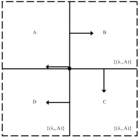
Proof: It is important to mention that k cannot exceed the number of boundary faces of A0 which are of di-mension dim A
( )
0 −1. Since the k paths are disjoint and non overlapping, each path has to start from a different face of A0. Without loss of generality, it is sufficient to prove the corollary for the case where k=2 and with paths consisting of single reduction pairs as shown in Figure 4. If we apply first the reduction by(
a A1, 1)
, then( )
1
0 1 0 0 1 1 1
1 1 , , where , P A a
A A A
A a
π = −λ λ = ∂ ∂
Applying the second reduction results in:
( )
(
)
( )
(
)
2 1 1
0 1 1 2
0 0 2
2 2
,
,
P P P
A A a
A A A
A a
λ
π π =π − ∂ −
∂
[image:8.595.194.433.639.706.2]Since P1 and P2 are disjoint non overlapping, it follows that a2 is not a face of A1, thus
( )
( )
( )
1 2
1 2
0 2
0 0 1 1 2 2 2
2 2
0 0 0
, , , P P P P A a
A A A A
A a
A A A
π = −λ −λ λ = ∂ ∂
= + Ψ + Ψ
Corollary 2. Let T be a reduction tree originating at A0, then the projection of A0 by T is equal to the sum of A0 and the projection chain of A0 by T.
Proof:
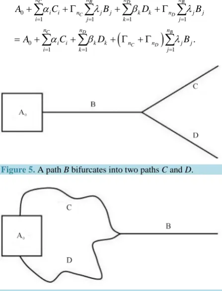
Typically, the trees originating at A0 can occur as pure paths, in which case the associated projections are given previously. Otherwise, we can find paths that share a common ancestral branch that originates at A0. This is seen as a bifurcation as shown in Figure 5. In this case, the ancestral branch is a path B:
(
b B1, 1)
,,(
bnB,BnB)
which is extended by two paths C:
(
c C1, 1)
,,(
cnC,CnC)
and D:(
d D1, 1)
,,(
dnD,DnD)
. The combination of the results in Theorem 9 and Corollary 1 can be used to show that the total projection of A0 by T =( ) ( )
BC , BDis given by
( )
0 01 1 1
C
B D
B n
n n
T i i n j j k k
i j k
A A B C D
π α β
= = =
= + Γ + Γ +
∑
∑
∑
The term
( )
0 0( )
01 1 1
C
B D
B n
n n
i i n j j k k T T
i j k
B α C β D π A A A
= = =
Γ + Γ + = − = Ψ
∑
∑
∑
is called the projection chain of the tree.In general, the tree can have many bifurcations at a given node and the bifurcations can occur at different nodes for which cases, the formula given above can be easily generalized.
One may wonder what happens when two paths are merging into a single path as illustrated inFigure 6. For this purpose, let’s consider the simple situation where two distinct reduction paths originating at A0 overlap at a
certain node, which is they are extended both by the same path.
In that situation, there are two independent pure paths CB and DB and the total projection of A0 is given as
follows
(
)
0
1 1 1 1
0
1 1 1
.
C B D B
C D
C D B
C D
n n n n
i i n j j k k n j j
i j k j
n n n
i i k k n n j j
i k j
A C B D B
A C D B
α λ β λ
α β λ
= = = =
= = =
+ + Γ + + Γ
= + + + Γ + Γ
∑
∑
∑
∑
∑
∑
∑
[image:9.595.202.426.414.708.2]Figure 5. A path B bifurcates into two paths C and D.
We see from the formula that it comes down to considering each path (which is also a tree) including the shared sibling branch as pure paths contributing to the projection of A0. This comes down to considering each
tree independently (see Figure 7).
Theorem 10. Let A0 be a cell adjacent to a RDAG in a chain complex C. The projection of A0 by the RDAG is equal to A0 to which we add the projection chains of A0 by all the trees in the RDAG that originate at A0, that is
( )
( )
0
0 0 0
A
RDAG T
T
A A A
π
∈ = +
∑
Ψ
where 0 A
is the collection of all the reduction trees in the RDAG originating at A0.
Proof: Since we deal with finite complexes the number of all possible trees starting at a given cell (here A0)
has to be finite. Thus, the results proved for paths in corollaries 1 and 2 and the subsequent remark regarding merging paths can be extended for the case of trees (splitting and merging) to find the formula for the projection of A0.
We review the projection formulas of paths and trees with the example of Figure 8. There are two trees TB
and TC originating at A0. The projection of A0 with respect to the tree TB can be written as
1 1B 2B2 3D1 4D2 4 1,
λ
+λ
+λ
+λ
+λ π
where π1=α1E1+α2E2+β1 1F +β2F2. The projection chain of A0 with respect to the tree TC is given by
1C1 2C2 3D1 4D2 4 2,
ϕ +ϕ +ϕ +ϕ +ϕ π
with π2 =µ1E1+µ2E2+σ1 1F +σ2F2. It follows that the total projection of A0 is given as the sum of both plus A0.
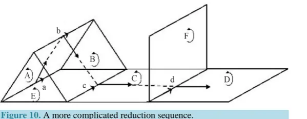
3.3. Why Acyclic Graphs
Adjacency alone does not guarantee that cycles are not created in a reduction DAG. To ensure that every reduc-tion sequence is associated with a well defined projecreduc-tion, we enforce acyclicity in the formed directed graphs. More generally, assuming that a reduction sequence
(
a A1, 1)
,,(
an,An)
is such that(
a A0, 0)
is adjacent to(
a A1, 1)
and(
an,An)
is adjacent to(
a A0, 0)
(see Figure 9), we consider extending the sequence to(
a A1, 1)
,,(
an+1,An+1)
by setting(
an+1,An+1) (
= a0,A0)
. However, the pair(
a A0, 0)
is not necessarilyad-missible since after performing the sequence of reductions
(
a A1, 1)
,,(
an,An)
, the cell A0 has been modifiedinto
A
0′
( )
0 0
1 1
1
i n
i
j i
i j
A A λ A
= =
′ = + −
∑
∏
and a0 =an+1 occurs in the boundary of A0′ as a face of both A0 and An. Its incidence number is therefore
calculated as follows
( )
0 0 0 0 0
1
, , 1 ,
n n
j n
j
A a A a λ A a
=
′
∂ = ∂ + − ∂
∏
which is not necessarily invertible. In Figure 9, ∂A a0′, 0 = − + −
( ) ( )
1 13× × × −(
1 1( )
1)
× =1 0 is not invertible which means that(
a A0, 0)
is not an admissible reduction pair. In our implementation, we avoid testing if [image:10.595.187.441.602.688.2]Figure 8. Example of reduction paths and the associated reduction DAG.
Figure 9. Cycles need to be avoided as reduction pairs are added in the tree.
reduction pairs are admissible or not by avoiding cycles as we build the reduction DAGs. This results in a more efficient algorithm.
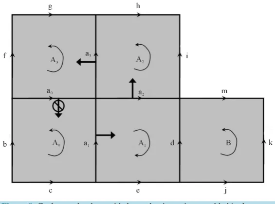
3.4. Using Projection Formulas
We recapitulate the formulas with a second example, see Figure 10. The first reduction pair is
(
a A,)
. Because the cell E is adjacent to the pair(
a A,)
, it is marked as a projected cell. In a list associated with the reduced cell A, we save the pair(
−λa,E)
where, 1 ,
a
E a A a
λ = ∂ = −
∂ . The reduction is continued from the faces of A. The second reduction pair is
(
b B,)
. We carry the information previously saved on the visited cofaces of b, so weadd
(
λ λb a,E)
, 1 ,b
A b B b
λ
∂
= =
∂
[image:11.595.171.454.332.542.2]Figure 10.A more complicated reduction sequence.
third reduction pair to be added is
(
c C,)
. The cell c is adjacent to both the reduced cell B and the projected cellE. From this point, we continue a path
(
(
a A,) (
, b B,) (
, c C,)
,)
and begin a sub-path(
(
c C,)
,)
. The in-formation saved with C considers the input of both paths. So we save(
−(
λcE+λ λ λcB b a)
,E)
where, 1 ,
cE
E c
C c
λ = ∂ = −
∂ and
, 1 ,
cB
B c
C c
λ = ∂ = −
∂ . But because the coefficients of contribution sum up to 0, it means
that C does not contribute to the projection of E. Thus, nothing is saved with C. The last reduction pair
(
d D,)
is added to the sequence. Because, d is adjacent to the unvisited cell F, F is marked as a projected cell. Thereduced cell C is also adjacent to d but no information was saved with C, so the only information to save with D
is
(
−λd,F)
where, 1 ,
d
F d
D d
λ = ∂ = −
∂ .
3.5. Building the Simplified Complex
Using reduction DAGs to compute the homology of a chain complex is a recursive process. At each recursion level, the algorithm simplifies the complex by constructing reduction DAGs on the complex and saving the as-sociated projections into appropriate data structures. This is performed simultaneously for each dimension. This process eventually stops when it is impossible to add another reduction pair to any reduction DAG. In that case, the algorithm will build the associated simplified complex and continue the reduction process on the simplified complex.
The simplified complex is rebuilt from the projected cells only (reduced cells are not considered). The boun-daries of the cells are updated using global projection formulas that allow to calculate the incidence numbers between cells of contiguous dimensions. Note that the reduced cells are not completely removed from the struc-tures since they may be needed to recover homology generators expressed in terms of cells of the original com-plex as we explain in subsection 3.8. Contrary to the classical case where the boundary updating is done at each reduction step and may concern cells that can be reduced at a later step, a major benefit of this new approach is that the boundary updating is done only among the projected cells which often constitute a small fraction of the number of cells in the original complex.
Continuing with the example used in Figure 10, we proceed to build its simplified complex. At this point from the projection formulas we have the projection of E, which is E′ = + +E A B and the projection of F
which is F′ = +F D. To build the simplified complex, we create two 2-dimensional cells, E′ and F′. We also create the projected lower dimensional cells (which is not illustrated in the example). Then, knowing that
F′ F D
∂ = ∂ + ∂ , we add the projected 1-cells in the boundary of D to the boundary of F′ using the correct coefficients. For example, if we suppose that d1 is a projected cell of dimension one that was in the boundary of D in the original complex. From the structures, we know that D appears in the projection of F with an inci-dence coefficient of 1 (F′ = +F D). So, we add d1 in the boundary of F′ with a coefficient of 1. This is done for all projected cells in all dimensions.
3.6. Performance Benefits of Using Reduction DAGs
coboundary of cells are maintained by lists data structures. Assuming ordered lists, the cost for merging two lists
1
L and L2 is bounded by O L
(
1 + L2)
, where L refers to the number of elements in L. Using unordered lists is bounded by O L(
1 ∗ L2)
.1) Classical Reduction Method
(a) Reduction
(
a A1, 1)
. According to step 2.a) of algorithm 2, we update cofaces of a1. That is, for each 2-cell β in the coboundary of a1, we add the set of cells in the boundary of A1 to the boundary of β using the right coefficient. Therefore, this operation costs an order of ∂ + ∂ = + =A1 A0 4 4 8 list updates.In step 2.b), we update the coboundaries of faces of A1. For each 1-cell α in the boundary of A1, we add the set of cells in the coboundary of a1 to the coboundary of α using the right coefficient. This time, the cost is in the order of
(
cobd +cobe + coba2 + ⋅3 coba1)
=11. Taken all together, it costs an order of 8 11 19+ = lists updates for the first reduction.(b) Reduction
(
a2,A2)
. Now ∂ = − + + + −A0 b c d e a2−a0, thus updating cofaces of a2 is in the order of(
∂A0 + ∂A2)
=(
6+4)
=10.For step 2.b), updating faces of A2 is in the order of
(
cobi +cobh+ coba3 + ⋅3 coba2)
=10. Taken together, the cost for the second reduction is in the order of 10 10+ =20 lists updates.(c) Reduction
(
a A3, 3)
. Now ∂ = − + + + + − −A0 b c d e i h a3−a0, and updating cofaces of a3 costs an order of ∂ + ∂ = + =A0 A3 8 4 12 lists updates.For step 2.b), updating faces of A3 amounts to a cost in the order of
(
cob f + cob g + coba0 + ⋅3 coba3)
=10.The total cost for the third reduction is in the order of 12 10+ =22.
Taken all together, the three reductions cost an order of 19+20+22=97 lists updates. Generally, as the re- ductions go on, the costs increase because the boundary and coboundary lists tend to grow in size.
2) Reduction DAGs Method
(a) Reduction
(
a A1, 1)
. The pair(
)
1, 0 a Aλ , where 1
0 1
1 1
, ,
a
A a A a
λ = − ∂
∂ is saved in a list maintained by A1. The
cost is one list update.
(b) Reduction
(
a A2, 2)
. The pair(
)
2 1, 0 a a Aλ λ , where 2
1 2
2 2
, ,
a
A a A a
λ = − ∂
∂ is saved in a list maintained by A2.
The cost is one list update.
(c) Reduction
(
a A3, 3)
. The pair(
)
3 2 1, 0 a a a Aλ λ λ where 3
2 3 3 3
,
,
a
A a
A a
λ = − ∂
∂ , is saved in a list maintained by
3
a . The cost is one list update.
(d) Reconstruction of the simplified complex. For each non reduced 1-cell a, we scan through its cofaces of the original complex and link a with the list of projected cells previously saved by using the right coefficients. The total cost is in the order of the number of remaining 1-cells plus the size of the lists of adjacent projected cells. Note that usually, the simplification process continues on the lower dimensions. So at the end there will remain only a fraction of the lower dimensional cells (here 1-cells). The Reduction DAGs method is more efficient as long as the cost for reconstructing the simplified complex is low which our experimental results corroborate.
3.7. Minimizing Lists Updates
Different reductions lead to different computational costs (measured by the number of lists updates). We attempt to achieve a good overall performance by choosing reduction pairs that should minimize the number of updates. To select among many candidate reduction pairs, we use a heuristic that estimates their respective costs. Given a reduction pair
(
a B,)
, this cost is approximated by the number of non reduced cofaces of a (other than B) plus the size of the projection lists of each reduced coface of a.We illustrate this on an example in Figure 11. Suppose that the 2-cell A is already reduced and has
(
λ1,A1)
3.8. Calculating Generators
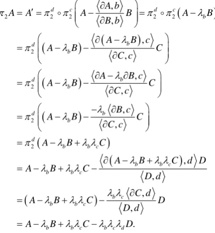
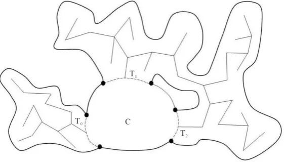
An interesting aspect of using the reduction DAGs method to compute homology is that the data structures allow to extract the homology generators at a low additional cost. We explain how to proceed. Let us consider the complex of a plane quotiented by its boundary as illustrated in Figure 12. This complex is homeomorphic to a 2-sphere and the 2-cell A represents the 2-generator A′ = +A
λ
1B+λ
2C+λ
3D. The generator associated to a projected cell corresponds to the projection of the cell. As we illustrated in Figure 12, after each reduction, the projection coefficientsλ
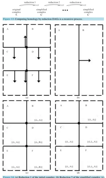
i are saved into the projection lists maintained in each reduced cell. Generally, once the complex has been simplified to the level where all boundaries are trivial, one has to examine all projected (non-reduced) cells and find their corresponding coefficients in the projection lists of the reduced cells. Thus, to get the 2-generator associated to the 2-cell A, one has to scan through each reduced 2-cell and extract the projec-tion coefficients associated to A. [image:14.595.199.428.309.451.2]However, computing homology by reduction DAGs is a recursive process (seeFigure 13) and this needs to be considered when calculating the generators. Projections correspond to generators but they can be expressed with cells of the simplified complex at any level of the recursion. However, in order for the generators to carry geometric meaning, it makes sense only to express the generators with cells from the original complex. Due to the recursive simplifications, a projected cell at a previous level of the recursion may become a reduced cell at a later level of the recursion. We illustrate this in Figure 14. In this example, there are two levels of recursion.
Figure 11.Cost of performing a reduction in terms of list updates.
[image:14.595.198.430.477.708.2]Figure 13.Computing homology by reduction DAGs is a recursive process.
(a) (b)
[image:15.595.131.497.82.698.2]
(c) (d)
The final simplified complex is obtained after reducing the vertical edge and the 2-cell B shown in Figure 14(b). At this step, the cell A represents a 2-generator that is expressed as A′′=A′+
λ
5B′ (considering that after the first reduction we rename the original cells A and B as A′ and B′). Note that in fact, the algorithm always works on the original cells and never copy nor create any new cell during the whole computation. Returning from the last recursion, we know that A′ = +A λ1C+λ2E and B′ = +Bλ
3D+λ
4F. The cell A represents a projected cell at both recursion levels (14(b) and 14(c)) and requires no special consideration. On the other hand, the cell B is a projected cell at the first level of recursion but becomes a reduced cell at the second recursion level. Consequently, returning from the second recursion level, we scan through each 2-cell and whenever B is encountered in one of the projection lists, it is replaced by λ5A. This is shown in Figure 14(d). Finally, the generator is expressed by A′′ = +A λ5B+λ1C+λ λ5 3D+λ2E+λ λ5 4F . In Figure 15 we show different 1- generators that we extracted from 3D models.3.9. What If Boundaries Are Not Trivial?
In previous subsections, we stressed that all boundaries have to be trivial in order to obtain homology and its generators at the end of the reduction process. But in practice, when all reductions are done we can be in a situation
(a) (b) (c)
[image:16.595.88.541.279.695.2]
(d) (e) (f)
where some of the boundaries remain non trivial. For example, this may be due to the presence of torsion. In Definition 1, the pair
(
a B,)
is defined as a reduction pair if ∂B a, = ±1. But this condition is in fact toorestrictive. In order for πd to be a group homomorphism, ,
,
c a B a
λ= ∂
∂ has to be an integer. This is satisfied when ∂B a, divides ∂c a, for every c∈Cd . The easiest and most efficient way to guarantee this is to choose B and a such that ∂B a, = ±1. Thus, for performance considerations, we designed the reduction DAGs algorithm to consider only reduction pairs with ±1 coefficients. But the drawback is that once all reductions are done, it is not guaranteed that all boundaries will be trivial. There may remain reduction pairs such that
, 1
B a
∂ ≠ ± but ∂B a, divides ∂c a, . In that case, one can modify the present algorithm to test for divisi-bility and continue the computations with the modified version. Another possidivisi-bility is to have recourse to a clas-sical algorithm such as the Smith Normal Form. Note that at this level most of the cells generating the complex have already been reduced to a small number.
4. Data Structures and Algorithms
The first data structure represents a chain complex.ChainComplex:
E: two dimensional array of cells organized by their respective dimension, that is E[d][i] denotes the i-th
d-cell.
In our implementation, the pointer to a cell is used to identify the cell. These identifiers are saved in E. The main benefit to using pointers is that when we build the simplified complex, no new cell is created. Only the pointers of the projected cells are copied into the simplified complex.
Cell:
boundary/coboundary: list of faces/cofaces.
state: a flag taking one of the values in {NORMAL, REDUCED, PROJECTED, VISITED}.
projCells: list to save the PROJECTED cells and their associated coefficients that project onto the given cell when it is REDUCED.
nbUpdates: approximates the number of updates to a projCells list when the given cell is reduced by one of its cofaces.
Initially, all cells are set to the NORMAL state. REDUCED is assigned to the cells in a reduction sequence and PROJECTED is assigned to the cells adjacent to a reduction sequence. The VISITED flag is assigned to the
d-cells that don’t have any
(
d+1)
coface that can form an admissible reduction pair. A reduction pair(
a B,)
is admissible if ∂B a, = ±1 and adding the pair to the reduction DAG does not create a cycle. The flag helps to avoid testing more than once if the given d-cells have an admissible reduction pair.The projCells list is used by the REDUCED cells to keep track of the coefficients of contribution of every PRO- JECTED cell for which it contributes. For example, if we use the sequence of reduction pairs illustrated in Figure
2, then B.projCells and C.projCells will respectively contain
(
λb,A)
and(
λ λb c,A)
where ,,
b
A b B b
λ = − ∂ ∂
and ,
,
c
B c C c
λ = − ∂ ∂ .
To build a sequence of reduction pairs, nbUpdates is used to select reduction pairs that should minimize the amount of updates to the projCells list. The number of updates is approximated by the number of non reduced cofaces plus the number of entries in the projCells lists of REDUCED cofaces.
We now give the principal steps of the algorithm.
HOM_RDAG(ChainComplex K) returns the Betti numbers of a chain complex K by using reduction DAGs. 1) (Initialization) For all cells in K, set its state to NORMAL, empty projCells, set nbUpdates to the number of cofaces.
2) (Reduce cells) Proceed by decreasing order of dimension. Order the d-cells by increasing value of nb- Updates. Following this order, start a reduction DAG (call BuildRDAG()) from each cell whose state is NOR- MAL.
3) (Build the simplified complex) Call BuildSimplifiedComplex(K). This method extracts the boundary infor-mation from the data structures to build a simplified complex K′.
Continue to recursively simplify K′ by calling HOM_RDAG(K′) until there are no reduction pair left. Test if all boundaries are trivial. If not, then continue the reduction process with another method such as SNF. 4) (Return the Betti numbers) Assign the number of PROJECTED d-cells to βd.
BuildRDAG(Cell c) builds a reduction DAG from cell c.
1) (Initialization) Save c.nbUpdates into nbUpdatesLimit for later use.
2) (Find a reduction pair) Find a coface B of c such that B is NORMAL or VISITED. If a coface B is found, then call PairCells(c, B), otherwise set c to VISITED and exit BuildRDAG().
3) (Expand the reduction DAG) Expand the reduction DAG (repeat step 2) from all NORMAL faces of B that have nbUpdates ≤nbUpdatesLimit. Proceed in a breadth first search approach.
PairCells(Cell c, Cell B) adds the reduction pair
(
c B,)
to the sequence and updates the data structures ac-cordingly.1) (Update projCells) For all cofaces C of c different than B, if C is REDUCED, then add λc∗C.projCells to
B.projCells. Otherwise, set C to PROJECTED and add λc∗C to B.projCells, where
, ,
c
C c B c
λ = − ∂ ∂ . 2) (Update the nbUpdates variable) For all faces a of B different than c, add
|B.projCells|-1 to c.nbUpdates. For all faces of c, remove one to nbUpdates.
BuildSimplifiedComplex(Complex K) extracts the boundary and coboundary information from the data structures to build a simplified complex K′.
Note: In the preceding methods, the coboundary list of a cell is never modified. Thus, when referring to co-faces, it is about the cofaces in the complex K at a given recursion level before any reduction is performed.
1) (Update boundary) Proceed by increasing order of dimension. Let c be a PROJECTED d-cell of K. For all cofaces C of c, iterate through C. projCells. Let B be a
(
d+1)
-cell in C. projCells andλ
B its associated coef-ficient. Add λB ∂C c c, to B.boundary and update c.coboundary accordingly.Finally, remove all REDUCED cells remaining in the boundary and coboundary of PROJECTED cells. Copy the pointers of all PROJECTED cells into K’.E.
5. Experimental Results
Because of its heuristic and recursive design, we had major difficulties to analyze the time complexity of our algorithm. Instead, we approached the problem by evaluating its performance on a wide range of experimenta-tions. We compared its performance with the reduction algorithm 2 on different data series: d-balls, d-spheres, tori, Bing’s houses, 3D medical scans and randomly generated d-complexes.
The series of d-balls and d-spheres were created by juxtaposing d dimensional cubes along each dimension. A 3-ball of size 10 is the cube obtained by placing side by side 10 × 10 × 10 3-cubes and making the correspond-ing identifications of lower dimensional cells. A d-sphere is a d -ball quotiented by its boundary. We also structed the tori and Bing’s houses from 3-cubes, although they are both 2 dimensional complexes. This con-struction does not affect the homology. We created two data series from 3D medical scans: brain and heart. Each of them is created from 3D images by selecting the pixels whose values are higher than a threshold. Lastly, we randomly generated d-complexes by choosing
(
d+1)
random numbers referring to the number of generators. We created a d-cell for each d-generator and randomly linked the d-cells to the(
d−1)
-cells. By subdivision, we obtained complexes of various data sizes.In the experimentation, we use the following terminology. A data series refers to one of d-balls, d-spheres, tori, Bing’s houses, 3D medical scans or randomly generated d-complexes. Each data series is constituted of many datasets. For example, d-balls contain the 2-ball, 3-ball, ..., 6-ball. Each dataset contains many files of complexes of various data sizes. For example, there are 15 files in the 2-ball data set for which the data size vary from 2000 up to 10,000,000. The size of a complex is measured as the number of cells plus the number of links (entries in boundary lists). A test is an execution of the algorithm on a file of a specified data set.
coboundary lists of all cells in the complex before each test.
We performed 30 tests for each file and computed the average, maximum and standard deviation of the time used for calculating the homology, the generators and sorting. We measured the sorting time because it has a time complexity of Θ ⋅
(
n logn)
and we wanted to verify that sorting would not monopolize the computation time. Also, we saved statistics on the number of recursions to see its influence on the global performance. Here we grouped and summarized the results per dataset. [image:19.595.85.540.243.377.2]We begin with our most interesting results (see Table 1) which compare the performance of the reduction DAGs algorithm with the classical reduction method on different datasets. We can observe a significant im-provement between the two methods. Knowing that the time complexity of the reduction method is quadratic (using ordered lists), those results suggest a subquadratic time complexity for the reduction DAGs algorithm which is what we measured inTable 2.
Table 1. Comparison of the reduction DAGs algorithm versus the classical reduction method.
Dataset Data Size Times Faster
3-Ball 115,905 195.4
4-Ball 27,841 147.3
2-Sphere 517,145 65.0
3-Sphere 134,777 182.5
Torus 418,608 36.0
Heart 545,492 50.5
3-Complex 265,322 410.0
5-Complex 431,186 458.8
8-Complex 330,285 185.9
Table 2. Approximated performance with respect to dataset, data size and dimension.
Equation Time (msec) Vs Data Size
Dataset N β α 104 105 106 107
2-Ball 15 9.05E−8 1.11 2.49 32.11 413.66 5329.04
3-Ball 11 4.63E−8 1.15 1.84 26.04 367.77 5194.95
4-Ball 11 4.26E−8 1.14 1.55 21.35 294.72 4068.27
5-Ball 9 5.66E−8 1.12 1.71 22.53 297.04 3915.76
6-Ball 5 3.56E−8 1.15 1.42 20.02 282.78 3994.39
2-Sphere 17 5.77E−8 1.18 3.03 45.83 693.71 10,499.67
3-Sphere 16 2.79E−8 1.22 2.12 35.12 582.91 9673.96
4-Sphere 10 3.38E−8 1.17 1.62 23.93 353.93 5235.00
5-Sphere 9 5.52E−8 1.14 2.00 27.67 381.89 5271.56
6-Sphere 5 3.30E−8 1.17 1.58 23.36 345.55 5111.09
7-Sphere 3 1.31E−8 1.24 1.19 20.76 360.80 6270.05
Torus 5 1.48E−7 1.07 2.82 33.13 389.28 4573.64
Bing’s House 5 2.18E−7 1.04 3.15 34.55 378.84 4153.90
Heart 6 6.84E−8 1.13 2.26 30.55 412.15 5559.76
Brain 6 3.13E−8 1.20 1.97 31.30 496.07 7862.20
2-Complex 9 6.78E−8 1.24 6.18 107.46 1867.37 32,451.12
3-Complex 9 7.89E−9 1.36 2.17 49.78 1140.45 26,126.25
4-Complex 9 2.82E−9 1.45 1.78 50.15 1413.35 39,833.56
5-Complex 9 4.95E−9 1.38 1.64 39.32 943.20 22,625.87
6-Complex 9 3.04E−9 1.41 1.33 34.11 876.75 22,535.83
7-Complex 9 2.42E−8 1.23 2.01 34.18 580.52 9858.60
[image:19.595.94.536.401.722.2]In Table 2 we report the approximative time that our algorithm uses to calculate homology on various data-sets. The second column (N) gives the number of files within the dataset. The third and fourth columns show the parameters
α
and β that best-fit the equation “ time≈ ⋅β data_sizeα“, where time is expressed in seconds. We obtained the best-fits from the times measured on the individual files of each dataset. In the last four col-umns, we present the times in milliseconds that we get from the best-fit equation for different data sizes. Those times approximate the real times that we measured in real experiments. For example, on 30 tests, we measured an average time of 4992.24 ms on a torus of size 10944304. The best-fit equation approximates a time of 4573.64 ms for a torus of size 10000000.From Table 2, we observe that α≈1.16 and β ≈5E−8 for d-balls and d-spheres without regard of the dimension. Except for few values,
α
is relatively constant while β gradually decreases as the dimension creases. We explain this by the fact that the ratio of exterior face reductions versus interior face reductions in-creases with the dimension. An exterior face reduction denotes a reduction pair(
a B,)
for which a has only the coface B in its coboundary list. On the other hand, we use the term interior face reduction when a is shared by more than one coface. Algorithmically speaking, an exterior face reduction is more advantageous because it does not cost any update to the projection lists, while an interior face reduction costs at least an update. [image:20.595.144.485.505.719.2]We observe that the approximation times and the parameters
α
and β for the heart and brain datasets, remain in the same order as those of d-balls and d-spheres despite the high numbers of generators as shown in Table 3. For example, the file heart96 had 30 connected components, 107 holes and 19 voids. For these two da-tasets, the number of generators was not a relevant factor for the performance of the algorithm. We think it is because those two datasets contain a high ratio of exterior face reductions, which cost near to nothing. If we compare with the random d-complexes then the topology is an important factor. Indeed, as the data size in-creased we observed bigger differences in the time performance.In Figure 16, we also reproduced the algorithm’s performance on the files of each dataset. We used a loga-rithmic scale on both axes to better distinguish the trends. In Figure 16(d), each file in a d-complex has a dis-tinct topology. It explains why we see only a weak trend in opposition to the other datasets where the trends are strong.
Another interesting aspect of the algorithm to consider is the number of recursions which is expressed as the number of reduction calls in Table 4. Interestingly, one reduction call was enough to calculate the homology of all d-balls, d-spheres and Bing’s houses. It means that the algorithm did not reconstruct an intermediate simpli-fied complex to obtain the homology. For other datasets, the algorithm had to reconstruct simplisimpli-fied complexes to carry out the computation. As an example, a value of n means that, on average, the algorithm constructed
(
n−1)
simplified complexes. The Max column shows the average of the maximum number of calls and the last column refers to the average standard deviation.Table 3. Number of generators of the files in the heart and brain datasets.
File Name Number of Generators
heart192 (11, 9, 0)
heart160 (4, 15, 2)
heart128 (39, 12, 6)
heart96 (30, 107, 19)
heart64 (38, 228, 104)
heart32 (111, 220, 208)
brain192 (11, 0, 0)
brain160 (109, 1, 0)
brain128 (230, 25, 0)
brain96 (255, 153, 4)
brain64 (134, 407, 21)
(a)
(c)
[image:22.595.88.540.76.692.2](d)