Performance Comparison of “Modified CO-DSEDF” with
CO-LALF for CO-Scheduling of Update and Control
Transactions of Real Time Data
Gauri Chavan
M.E. Student,
Electronics Department, Shah and Anchor Kutchhi Engineering College, Chembur, Mumbai, India.
Vidya Gogate
Assistant Professor,
Electronics Department, Shah and Anchor Kutchhi Engineering College, Chembur, Mumbai,
India.
ABSTRACT
Real time system is the system where data should be processed in time. The real time data is stored in real time database within the specified time interval. This time interval is called as validity time interval [1],[2]. The validity of real time data is maintained using different scheduling algorithms. The process of maintaining the validity of real time data is done by using several update transactions. The appropriate scheduling algorithm is used to schedule the number of update transactions. The different algorithms used to maintain the validity of real time data are Earliest deadline First (EDF), Deferrable scheduling with Earliest Deadline First (DS-EDF), Deferrable scheduling with Least Actual Laxity First (DS-LALF) [3],[4],[5]. The real-time data stored in real-time database is compared with some predefined value [8]. If the stored data value is not equal to the predefined value then control transactions are generated. Therefore update and control transactions are needed to be scheduled in such a way that both the transactions meet their deadline constraints. In literature the CO-Scheduling with Least Actual Laxity First (CO-LALF) algorithm is used to schedule update and control transactions [5]. After studying different algorithms we need to propose the CO-scheduling with Deferrable scheduling with Earliest Deadline First algorithm (CO-DSEDF) to schedule the update and control transactions. DS-EDF and DS-LALF give high priority to update transactions [4],[5]. So quality of data is maximized [4]. To maximize the quality of data & the quality of control coscheduling algorithms CO-DSEDF & CO-LALF are used. These algorithms are used to schedule update & control transactions. So quality of data and quality of control are maximized [5]. We worked out different problems to compare the performance of CO-DSEDF with CO-LALF. We have checked the feasibility of the scheduling algorithms for various scheduling problems to maintain the data freshness. We also present the estimation of processor utilization and context switching for CO-DSEDF & CO-LALF.
Keywords
Validity time, real-time database, Data freshness, CO-Scheduling, update and control transactions, response time
1.
INTRODUCTION
In real-time system timing constraints are important to process any data. The data value is bounded by some time interval. If the data processing does not take place within the validity time interval then real time system is invalid. So to have processing of data dynamically, different scheduling algorithms are used. For example, data generated by a temperature sensor.
Temperature sensor transmits sampled data to the controller every 100 milliseconds (ms) [8],[11]. So the specified time interval to send next update transaction is before 100 ms. Each sampled value of data is associated with the update transactions. There are several update transactions and each update transaction has number of jobs. The specified time interval to send next update transaction is called the validity time of data [1]. If data is not updated before the validity time then that data is called as stale data. So it is essential to maintain the validity of this data as it is used for further processing. The process of maintaining the real-time data valid is called as real-time data freshness and the valid data is called as fresh data [2]. The different update transactions are used to store the real time data in real-time database (RTDBs) [6],[12]. The data value stored in RTDB is compared with the threshold value. If the data value stored in RTDB is more than the designed threshold value then control transactions are generated [5],[11]. The scheduling of such update and control transactions together in a real time system is called as co-scheduling [5]. Different scheduling algorithms are used to schedule the update transactions in such a way that it meets its deadline constraints. The algorithms are EDF, DS-EDF, DS-LALF are used to maximize the quality of data[4]. CO-DSEDF & CO-LALF are co-scheduling algorithms used to schedule the update as well as control transactions to meet its deadline constraints. These algorithms maximized the quality of data and the quality of control. We have compared the performance of CO-DSEDF and CO-LALF by using different scheduling problems to check the schedulability of the problem for the given algorithm We have done the estimation of processor utilization and context switching for each algorithm. We have used TORSCHE scheduling toolbox to plot the schedule of different transactions [14]. We have worked out the different scheduling problems with different requirements. & shown that the processor utilization is reduced for CO-DSEDF than CO-LALF.
2.
SYSTEM MODEL
generated by the embedded processor. These signals are called as control transactions. The control transactions act as input to the actuator. Actuator is a device that takes inputs from the embedded system and converts into electrical signal to have corrective action on its environment [11]. The physical quantities like temperature, pressure, flow are to be measured for the given system. As shown in fig.1 the sensors of the real time computer collect data from the environment and stores in Real time Database using update transactions [6]. The embedded system compares the data in RTDB with the designed threshold level and generates control signals. The embedded processor sends information to the actuators so that actuators can carry out the required operation on the environment [8], [9]. Real time operating system is the main part of the real time embedded system. Scheduling is the main function of RTOS kernel. Scheduler schedules the task to have the proper order of execution of each task to meet its deadline.
Fig: 1 System Model
2.1
Real time Data-base (RTDB)
In real-time applications we need to store large amount of data. This data is processed for further operation [12]. The stored data is used for controlling the input parameters. The examples of such a system are process control system, Internet service Management, spacecraft Control system, Network Management System [7]. Real-time database is associated with the timing constraints. The basic requirement of Real-time database is the transaction deadline. If the data in real-time database gets updated before the deadline then we get the valid data. Real-time database makes use of different scheduling algorithms to update the data. The state of the RTDB is changing continuously [13].The data should be updated dynamically to have the correct results. The sensor or input device monitors the state of the physical system and updates the database with new information. This new information must be updated time to time or in the given validity interval. Examples of such RTDBs are railway reservation system; spacecraft control system, internet service management [7]. In real-time system large amount of data is handled at a time. For example an air traffic control system constantly monitors hundreds of aircrafts. Depending on the data stored such as fuel, altitude & speed, the real time system makes decisions about incoming flight paths and determines the order in which aircraft should land [7].The other examples are online railway reservation system, patient monitoring system. In these systems also real-time databases get updated time to time to avoid the failure of real-time system.
2.2
Update and Control Transactions
In real-time system different transactions are generated from different sensor inputs. Each transaction is having its own validity time interval. The transactions are used to update the real-time data in Real-time database are called as update
transactions. System model shows a real time sensing and control system.
Tui : ith update transaction, i = 1 to n
Ji,j : j number of jobs of ith transaction, j = 0 to m.
Tcp: pth Control transaction, p= 1 to t
Jcpq : q number of jobs of p th
transaction, q= 0 to v
The system consists of a fixed set of update transactions denoted as Tui where i= 1 to n. Each transaction is having n
number of jobs which are denoted as Ji,j [4],[5]. For example
transaction1, Tu1 is having m number of jobs, each of the job is
denoted as J11, J12, J13,………J1m. The update transactions are
used to maintain the validity of data so these transactions are updated before the validity interval expires. Each job Ji,m of
transaction Tui is updated depending upon the scheduling
algorithm used, to meet its deadline constraints. Each updated job stored the new data value in RTDB. The real time controller depending upon the application strategies compares the values of each update transaction with the designed threshold value. If data value exceeds than the threshold level then the control transactions are generated denoted as Tcp, where p= 1 to t.
Control transactions can have q number of jobs. For example Tc1 has q jobs Jc11Jc12,………Jc1q [5]. The scheduling of update
and control transactions together is called as co-scheduling. Different scheduling algorithms are used to meet the deadline of update & control transactions. If any of the update job is missing its deadline then real-time system gets failed. So to have the accurate results of real-time system, the update and control transactions should meet its deadline constraints.
3.
TORSCHE SCHEDULING TOOLBOX
TORSCHE (Time Optimization of Resources, Scheduling) is a MATLAB-based toolbox used to show the scheduling of different algorithms for off-line & on-line scheduling problems [14]. Task, TaskSet and Problem are the main objects of TORSCHE. The Task is a data structure; it includes all parameters of the task. These parameters are processing time, release date, deadline etc. If tasks are grouped then it forms Taskset. The Problem is a small structure describing classification of deterministic scheduling problems. Each task or job has it own parameters. By defining suitable scheduling algorithm, we can plot schedule of the required algorithm in MATLAB [14].
The steps to plot schedule of the given scheduling problem is as shown below:
1. First create task object
t1 = task ([Name,] ProcTime [, ReleaseTime [, Deadline [, DueDate [, Weight [, Processor]]]]])
2. Create TaskSet Object
T = [t1 t2 t3], T1 consists of number of tasks or jobs for the given scheduling problem. T1 is TaskSet Object [14].
3. Define the problem
prob = problem(‟P|prec|Cmax‟)
The problem consists of three parts. The first part „P‟ describes the processor that in uniprocessor or multiprocessor environment. The second part „prec‟ describes precedence constraints & third part „Cmax‟ describes the optimality criterion [14].
4. Structure of scheduling Problem
„name‟ is the name of the algorithm. The „T‟ is TaskSet object which contains tasks or jobs to be scheduled. The „problem‟ describes the classification of deterministic scheduling problem. The „processors‟ define the number of processors. The ‟parameters‟ define additional information for algorithms [14].
5. Plot the schedule
PLOT (TS), it gives schedule of all tasks or jobs defined in TS for the given algorithm [14].
4.
ALGORITHMS
Input: Number of Update Transactions, Validity time and execution time of each update transaction, number of jobs in each update transaction, release time and deadline time of each job.
Output: Schedule of the input transactions job.
4.1
Deferrable Scheduling with Earliest
Deadline First (DS-EDF)
1. Input number of update transactions with its validity time and execution time.
2. Input number of jobs in each transaction with its release time and deadline time.
3. The deadline of next update job of same transaction is calculated using following formula
Next update job deadline, di, j+1= r i, j + Vi
4. Sort all update jobs in ascending order of deadline using following function:
sortAscending(); goto step 9 5. For (i=0; i < no_of_jobs; i++)
Create the array of jobs having deadline < next job deadline.
6. For (j=0; j < count; j++)
If (Jj .d > Ji.d) Put this job in hp_ctime.
7. Calculate new release time for Ji.
reltime = calReleaseTime(); 8. calReleaseTime()
calRelime= te - ctime – hp_ctime[i]
9. sort Ascending()
for (i=0; i < no_of jobs; i++)
if [( ji.r =Ji+1.r) || (Ji.r = Ji+1,r && Jid > Ji+1.d)]
swap Ji and Ji+1.
4.2
Deferrable Scheduling with Least
Actual Laxity First (DS-LALF)
1. Input number of update transactions with its validity time and execution time.
2. Input number of update jobs in each transaction with its release time and deadline time.
3. The deadline of next update job of same transaction is calculated using following formula
Next update job deadline, di, j+1 = r i, j + Vi.
4. Sort all update jobs in ascending order of deadline
using following function: sortAscending () ; goto step 8.
5. Group the job having release time = i and calculate new release time.
Ji,j.laxity = calnewRelTime(); goto step 9.
6. Set priority as per new release time. setpriority (); goto step 10
7. Process the first job and set the start and end time of job.
8. sortAscending()
for (i=0; i <no_of_jobs ; i++)
if [(Ji.r = Ji+1.r) || (Ji.r = Ji+1 .r && Ji.d > Ji+1 .d )],
Swap Ji & Ji+1.
9. calnewRelTime();
tempjob.r = tempjob.d - timer - tempjob.ctime. 10. setpriority()
check Ji.laxity & Ji+1.laxity with respect to Ji.d.
4.3
Co-scheduling with Least Actual Laxity
First (CO-LALF)
1. Input number of update transactions with its validity time and execution time.
2. Input number of update jobs in each transaction with its release time and deadline time.
3. The deadline of next update job of same transaction is calculated using following formula
Next update job deadline, di, j+1 = r i, j + Vi.
4. Input if any control transactions are generated as Tc
and its control jobs as Jc
5. Sort all update jobs and control jobs in ascending order of deadline using following function:
sortAscending() ;
6. Group the job having release time = i and calculate new release time.
Ji,j.laxity = calnewRelTime();
7. Set priority as per new release time. setpriority (); goto step 10
8. Process the first job and set the start and end time of job.
9. sortAscending()
for (i=0; i <no_of_jobs ; i++)
if [(Ji.r = Ji+1.r) || (Ji.r = Ji+1 .r && Ji.d > Ji+1 .d)],
Swap Ji & Ji+1.
10. calnewRelTime();
tempjob.r = tempjob.d - timer - tempjob.ctime. 11. setpriority()
4.4
Proposed Modified Algorithm:
Co-Scheduling with Deferrable Co-Scheduling
with Earliest Deadline First (CO-DSEDF)
1. Input number of update transactions with its validity time and execution time.
2. Input number of update jobs in each transaction with its release time and deadline time.
3. The deadline of next update job of same transaction is calculated using following formula
Next update job deadline, di, j+1 = r i, j + Vi.
4. Input if any control transactions are generated as Tc
and its control jobs as Jc
5. Sort all update jobs and control jobs in ascending order of deadline using following function:
sortAscending();
6. For (i=0; i < no_of_jobs; i++)
Create the array of jobs having deadline < next job deadline.
7. For (j=0; j < count; j++)
If (Jj .d > Ji.d) Put this job in hp_ctime.
8. Calculate new release time for Ji.
reltime = calReleaseTime(); 9. calReleaseTime()
calRelime= te - ctime – hp_ctime[i]
10. sort Ascending()
for (i=0; i < no_of jobs; i++)
if [( ji.r =Ji+1.r) || (Ji.r = Ji+1,r && Jid > Ji+1.d)]
swap Ji and Ji+1.
5.
RESULT AND ANALYSIS
5.1
Design of various Problems
1. There are n numbers of update transactions. Each update transaction „i „is having its own validity time Vi and
computation time Ci.
2. Each update transaction is having m number of jobs Ji,m.
Job Ji,m of ith update transaction is represented with two
parameters. These parameters are release time ri,j and deadline
time di,j.
3. The first job of each update transaction is having zero release time and respective validity time is used as a deadline. 4. The deadline of next update job is derived using this formula: di,j+1 = ri,j + Vi.
5. The control trasanctions are generated at any time. The job of control transaction is having release time and deadline time [5].
[image:4.595.316.544.74.160.2]5.2
Scheduling of Update Transactions
using DS-EDF and DS-LALF Algorithms
The different problems are given in table1 and 4 are worked out to check the feasibility of scheduling algorithms.Table 1. Problem Statement I
Tu1 Tu2 Tu3
V1=8, C1 = 2 V2=20, C2 = 3 V3=50, C3= 3
J10 (0,8), J11 (5, 8),
J12 (10, 13)
J20 (0, 20),
J21 (16, 20)
J30 (0,50).
Figure 2 shows the schedule for Deferrable scheduling with Earliest Deadline First Algorithm (DS-EDF). In DS-EDF algorithm, the new release time is calculated by considering the deadline constraints. The jobs are deferred to meet its deadline. Job, J30 has its new releasetimeas 47 because it does
not have any other job and all jobs of first and second update transactions are completed at 20 time units. The schedule of Deferrable Scheduling with Least Actual Laxity First (DS-LALF) for problem I is shown in fig. 3. In this figure by using DS-LALF, the new release time is calculated by considering the least laxity of each job. The update job with least laxity is scheduled first. All jobs meet its deadline as shown in fig. 3 till 19 time units. Jobs with least laxity, preempt the job with greater laxity. Jobs with same release time are inserted into queue initially. The laxity of each job is calculated and jobs are arranged in ascending order of Laxity. At each time unit new release jobs are inserted into queue and laxity of each job is calculated and arrange in ascending order of Laxity.
Fig: 2 Schedule of Example I using DS-EDF
Table 2. DS-EDF Result for Example I
Number of Jobs
Schedulability Context Switching
Processor Utilization
6 Yes 0 0.3
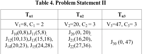
[image:4.595.316.543.358.618.2]Table 4. Problem Statement II
Tu1 Tu2 Tu3
V1=8, C1 = 2 V2=20, C2 = 3 V3=47, C3= 3
J10(0,8),J11(5,8),
J12(10,13),J13(15,18),
J14(20,23), J15(24,28).
J20 (0, 20),
J21(16,20),
J22(27,36).
J30 (0, 47)
In problem II we have increased number of jobs in each update transaction, in first update transaction Tu1, from 3 to 6
update jobs and in second update transaction Tu2, from 2 to 3
update jobs. Figure 4 gives the scheduling of Example II by using DS-EDF algorithm. By using DS-EDF algorithm, the new release time is calculated in such a way that all update jobs meets its deadline and we can maintain the data validity. Figure 4 & 5 give the schedule of problem II using DS-EDF & DS-LALF algorithm. But in problem II, the scheduling using DS-EDF is not meeting its deadline constraint for job J21.The update job J11 is completing its execution at 21 but J21
should be completed at 20. So J21 missing its deadline by 1
[image:5.595.53.283.73.160.2]time unit. So data validity is not maintained. To maintain the data validity the next algorithm DS-LALF is used to schedule same transactions shown in problem II. The scheduling of problem II using DS-LALF is shown in fig. 5. In this algorithm the least laxity is calculated so that the update job with the least laxity is scheduled first.
Fig: 3 Schedule of Example I using DS-LALF
Table 3. DS-LALF Result for Problem I
Number of Jobs
Schedulability Context Switching
Processor Utilization
6 Yes 0 0.789
Fig: 4 Schedule of Example II using DS-EDF
Table 5. DS-EDF Result for Problem II
Number of Jobs
Schedulability Context Switching
Processor Utilization
10 No 0 0.51
As shown in figure 5, update job J21 is meeting its deadline
using DS-LALF. Job J21 completes at 20. So data validity is
[image:5.595.55.282.363.706.2]maintained using DS-LALF than DS-EDF in problem II. Therefore we can check the schedule of update jobs by using DS-EDF and DS-LALF algorithm. Depending on the given problem we can use any one algorithm which gives the schedule without missing its deadline.
[image:5.595.317.544.486.738.2]Table 6. DS-LALF Result for Problem II
Number of Jobs
Schedulability Context Switching
Processor Utilization
10 Yes 0 0.8
In Example II, the processor utilization in terms of update workload is more in DS-LALF. But the schedulability of the problem is not given by DS-EDF algorithm. The context switching is zero in both algorithms. The data validity is not maintained using DS-EDF algorithm. The DS-LALF algorithm maintains the data validity.
5.3
CO-Scheduling of Update and Control
Transactions using Modified Algorithm
CO-DSEDF and CO-LALF
[image:6.595.52.280.89.128.2]The different problems as given in table 7, 10 & 13 are worked out to check the feasibility of scheduling algorithms. These problems are worked for different transactions.
Table 7. Problem Statement III
Tu1 Tc1
V1=7, C1 = 2 C2 =2
J10 (0,7), J11 (4, 7),
J12 (8, 11)
Jc10 (3, 8).
[image:6.595.86.252.285.354.2]In problem III, we have considered update and control transactions. Figure 6 & 7 give the schedule of CO-DSEDF & CO-LALF respectively. The CO-DSEDF and CO-LALF algorithms meet the deadline constraints of update and control transactions. So the real-time data validity is maintained. The control transaction is also meeting its deadline so that the corrective action can take place to avoid any hazards of real-time system. The processor utilization for the update workload and to schedule the control transaction is more in DS-LALF than DS-EDF algorithm. The context switching is zero for CO-DSEDF & CO-LALF algorithm for the problem III. Figure 8 & 9 give the schedule of example IV for DSEDF & CO-LALF algorithm. In example IV we have increased the number of jobs.
Fig: 6 Schedule of Example III using CO-DSEDF
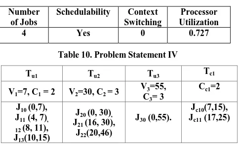
Table 8. CO-DSEDF Result for Problem III
Number of Jobs
Schedulability Context Switching
Processor Utilization
4 Yes 0 0.727
Table 10. Problem Statement IV
Tu1 Tu2 Tu3 Tc1
V1=7, C1 = 2 V2=30, C2 = 3
V3=55,
C3= 3
Cc1=2
J10 (0,7),
J11 (4, 7), 12 (8, 11),
J13(10,15)
J20 (0, 30),
J21 (16, 30),
J22(20,46)
J30 (0,55).
Jc10(7,15),
Jc11 (17,25)
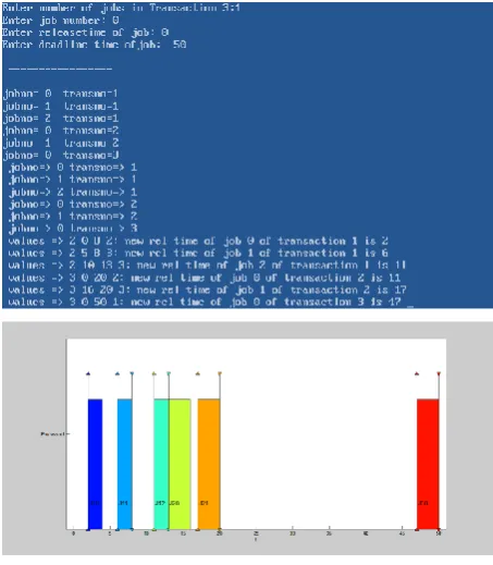
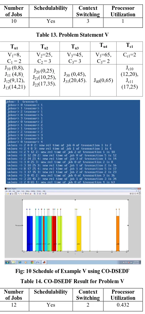
[image:6.595.316.543.491.749.2]The CO-LALF and DS-EDF algorithm meet its deadline constraints for update & control transactions. Therefore the real-time data validity is maintained and corrective action take place within the timing constraints. The context switching is more in CO-LALF than CO-DSEDF. The processor utilization for the update workload of update transaction and to schedule the control transactions is more in CO-LALF than CO-DSEDF. To minimize the power consumption of the processor we can use CO-DSEDF. As numbers of jobs are increased the processor utilization is reduced in CO-DSEDF as compared to problem III. The context switching for any real-time application should be as low as possible to have most accurate results of the real-time system. Figure 10 & 11 show the schedule of problem V using CO-DSEDF & CO-LALF respectively. Both algorithms give proper scheduling of update & control transactions. So data validity is maintained and the corrective action takes place before the validity interval expires. In Co-DSEDF we get number of free timeslots as compared to CO-LALF algorithm. The context switching is also increased in LALF than CO-DSEDF for the same problem. All the update and control transactions meet their deadline constraints and maintain the quality of data and the quality of control. We have worked out CO-DSEDF & CO-LALF algorithms for various problems and done the comparative analysis which is given in table 1.
[image:6.595.57.284.508.753.2]Table 9. CO-LALF Result for Problem III
Number of Jobs
Schedulability Context Switching
Processor Utilization
[image:7.595.311.546.81.590.2]6 Yes 0 0.8
[image:7.595.45.286.90.703.2]Fig: 8 Schedule of Example IV using CO-DSEDF
Table 11. CO-DSEDF Result for Problem IV
Number of Jobs
Schedulability Context Switching
Processor Utilization
6 Yes 0 0.8
Fig: 9 Schedule of Example IV using CO-LALF
Table 12. CO-LALF Result for Problem IV
Number of Jobs
Schedulability Context Switching
Processor Utilization
10 Yes 3 1
Table 13. Problem Statement V
Tu1 Tu2 Tu3 Tu4 Tc1
V1=8,
C1 = 2
V2=25,
C2 = 3
V3=45,
C3= 3
V3=65,
C3= 2
Cc1=2
J10 (0,8),
J11 (4,8),
J12(9,12),
J13(14,21)
J20 (0,25),
J21(10,25),
J22(17,35).
J30 (0,45),
J31(20,45). J40(0,65)
Jc10
(12,20), Jc11
(17,25)
Fig: 10 Schedule of Example V using CO-DSEDF
Table 14. CO-DSEDF Result for Problem V
Number of Jobs
Schedulability Context Switching
Processor Utilization
12 Yes 2 0.432
[image:7.595.47.282.443.746.2]Fig: 11 Schedule of Example V using CO-LALF
Table 15. CO-LALF Result for Problem V
Number of Jobs
Schedulability Context Switching
Processor Utilization
[image:8.595.55.285.71.406.2]12 Yes 3 1
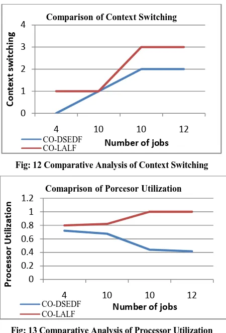
Table 16. Comparison Parameters
Number
of Jobs 4
10 10 12
Context Switching
CO-DSEDF 0 1 2 2
CO-LALF 1 1 3 3
Processor Utilization
CO-DSEDF 0.72 0.676 0.44 0.415
CO-LALF 0.8 0.821 1 1
In context switching low priority task is pre-empted and resume later. If number of context switching is there then it may degrade the performance of real-time system. Figure 13 shows the processor utilization of CO-DSEDF & CO-LALF. The processor utilization of DSEDF is less as compared to CO-LALF algorithm. So it reduces the power consumption of the processor. As the numbers of jobs are increased the processor utilization is reduced in CO-DSEDF. But In CO-LALF, as the numbers of jobs are increased processor utilization is increased. The processor utilization for the update workload of different jobs is estimated for different problems. If numbers of free slots are more in the scheduling of different tasks then processor utilization is reduced, though the numbers of jobs are increased.
Fig: 12 Comparative Analysis of Context Switching
Fig: 13 Comparative Analysis of Processor Utilization
6.
CONCLUSION
The DS-EDF and DS-LALF algorithms are used to schedule the update transactions. These algorithms are used to maintain the validity of real time data. If any of the algorithms is missing its deadline then real-time data validity is not maintained. So that the real time data updated in real-time database is stale or invalid data. To check the validity of data, different algorithms are worked out using different problems. DS-EDF & DS-LALF are used for update transactions while CO-LALF & modified algorithm, CO-DSEDF are used for update as well as control transactions. We have compared these algorithm using three different criteria for the same problem statement. These criterions are schedulability, context switching, and processor utilization in terms of update workload. In modified CO-DSEDF we get less context switching and less power consumption than CO-LALF. As numbers of jobs are increased, the processor utilization for the update workload is also increased in CO-LALF which is not feasible to minimize the power consumption of the processor. We have worked out these algorithms with uniprocessor system. In future we have to extend these algorithms to multiprocessor system where the performance measure parameters like resource sharing will make the system more complex. In CO-DSEDF, numbers of free time slots are also available which can be utilized by other jobs.
7.
REFERENCES
[1] M. Xiong, S. Han, K.-Y. Lam, and D. Chen, “Deferrable “Scheduling for Maintaining Real-Time Data Freshness: Algorithms, Analysis, and Results,” IEEE Transaction Computers, vol. 57, no. 7, pp. 952-964, July 2008.
0 1 2 3 4
4 10 10 12
Co
n
te
xt
swi
tc
h
in
g
Number of jobs
Comparison of Context Switching
CO-DSEDF CO-LALF
0 0.2 0.4 0.6 0.8 1 1.2
4 10 10 12
Pr
o
ce
ssor
Uti
lization
Number of jobs
Comaprison of Porcesor Utilization
[image:8.595.319.539.73.217.2][2] “A schedulability Analysis of deferrable scheduling Using Patterns” ,by Song Han, Deji Chen,Ming Xiong, Euromicro Conference on Real-time systems,IEEE2008. [3] S. Han, D. Chen, M. Xiong, K.-Y. Lam, A.K. Mok, , and
K.Ramamritham, “Schedulability Analysis of Deferrable Data Freshness, Technical Report TR-11- 38TR- 2055. pdf, 2011.
[4] “Schedulability Analysis of Deferrable Scheduling Algorithms for maintaining Real-time Data Freshness”, Song Han, Deji Chen, Ming Xiong, KAm-yiu Lam, Aloysius K. Mok, Krithi Ramamritham, IEEE TRASNACTIONS ON COMPUTERS,2012.
[5] “On Co-Scheduling of Update and Control Transactions in Real-Time Sensing and Control Systems: Algorithms, Analysis, and Performance ” by Song Han, Member, IEEE, Kam-Yiu Lam, Member, IEEE, Jiantao Wang, Student Member, IEEE, Krithi Ramamritham, Fellow, IEEE, IEEE TRANSACTIONS OCTOBER 2013. [6] “An essay on Real-time Databases”, by Raul Barbosa,
Department of Chalmers University of technology, Sweden.
[7] “An overview of Real-time Database Systems”, by Ben Kuo and Hector Garcia-Molina, Princeton University USA.
[8] “Managing Deadline Miss ratio & sensor Data Freshness in Real-time Daabases”, By Kyoung-Don Kang, Sang H. Son, IEEE transactions, VOL. 16,No. 10,October 2004. [9] ”Real-Time Systems” by Jane W.S. Liu, Pearson
Education.
[10]”Real-Time Systems” by C.M.Krishna & Kang G. Shin, Tata McGraw-Hill.
[11]“Process Control: Concepts, Dynamics & Applications: By S.K. Singh, PHI.
[12]An overview of real-time database systems Ben Kao and hector Garcia-Molina.
[13]”Value-Based Scheduling in Real-Time Database Systems” Jayant R. Haritsa, Michael J. Carey, and Miron Livny.