Modeling and Simulation for High Energy
Sub-Nuclear Interactions Using
Evolutionary Computation Technique
Mahmoud Y. El-Bakry1, El-Sayed A. El-Dahshan2,3, Amr Radi3,4, Mohamed Tantawy1, Moaaz A. Moussa1,5
1Department of Physics, Faculty of Sciences, Ain Shams University, Cairo, Egypt 2Egyptian E-Learning University, Giza, Egypt
3Department of Physics, Faculty of Education, Ain Shams University, Cairo, Egypt 4The British University in Egypt (BUE), Cairo, Egypt
5Buraydah Colleges, East Qassim University, Buraydah, KSA
Received 19 November 2015; accepted 10 January 2016; published 13 January 2016
Copyright © 2016 by authors and Scientific Research Publishing Inc.
This work is licensed under the Creative Commons Attribution International License (CC BY).
http://creativecommons.org/licenses/by/4.0/
Abstract
High energy sub-nuclear interactions are a good tool to dive deeply in the core of the particles to recognize their structures and the forces governed. The current article focuses on using one of the evolutionary computation techniques, the so-called genetic programming (GP), to model the ha-dron nucleus (h-A) interactions through discovering functions. In this article, GP is used to simu-late the rapidity distribution
N
N Y
1 d
d of total charged, positive and negative pions for p
−-Ar and
p−-Xe interactions at 200 GeV/c and charged particles for p-pb collision at 5.02 TeV. We have done
so many runs to select the best runs of the GP program and finally obtained the rapidity distribu-tion
N
N Y
1 d
d as a function of the lab momentum
(
PLab)
, mass number (A) and the number ofparticles per unit solid angle (Y). In all cases studied, we compared our seven discovered functions produced by GP technique with the corresponding experimental data and the excellent matching was so clear.
Keywords
1. Introduction
Evolutionary computation refers to a class of algorithms that utilize simulated evolution to some degree as a means to solve a variety of problems, from numerical optimization to symbolic logic. By simulated evolution, we mean that the algorithms have the ability to evolve a population of potential solutions such that weaker solu-tions are removed and replaced with incrementally stronger (better) solusolu-tions. In other words, the algorithms follow the principle of natural selection. Each of the algorithms has some amount of biological plausibility, and is based on evolution or the simulation of natural systems [1]-[8].
In 1990s, John Koza [9] [10] introduced the subfield called Genetic Programming. This is considered a sub-field because it fundamentally relies on the core genetic algorithm created by Holland [11], and differs in the underlying representation of the solutions to be evolved. Instead of using bit-strings (as with genetic algorithms) or real-values (as is the case for evolutionary programming [1]-[7] or evolutionary strategies [1]-[7], genetic programming relies on S-expressions (program trees) as the encoding scheme.
Hadron-nucleus (h-A) interactions have been considered as a corner stone in high energy physics because of its theoretical and practical interesting features and also it is an intermediate state between hadron-hadron (h-h) and nucleus-nucleus (N-N) interactions. So, there are a lot of models that concern the study of the hadron struc-ture [12]-[16] and the interactions between hadrons and nuclei such as the three-fireball model [17], quark mod-els [18]-[20], fragmentation model [21]-[23] and many more.
In our previous works [24]-[27], our group studied the applications of artificial intelligence and the evolutio-nary computation techniques such as neural network, adaptive fuzzy inference system, genetic programming, genetic algorithm, hybrid technique model and many others to solve many complex (nonlinear) problems in high energy physics and showed best fitting with the corresponding experimental data in comparison with the con-ventional techniques.
The study of hadron-nucleus interaction at high and ultrahigh energy has been a subject of great interest to high energy physicist because the nuclei provide a number of unique physics opportunities which are not availa-ble in elementary particle collisions [28].
In this article, Genetic programming (GP) model has been used to discover a function that computes the ra-pidity distribution of created (total charged, positive and negative) pions for p−-Ar and p−-Xe collisions at 200 GeV/c [29]-[31] and charged particles for p-pb collision at 5.02 TeV [32]. The seven discovered functions pro-duced by GP model show an excellent matching when they have been compared to the corresponding experi-mental data [29]-[32]. This article is organized as follows; Section 2 gives the definition and the outlines to the basics of the GP technique. Section 3 reviews the implementation of GP. Finally, the results and conclusions are provided in Sections 4 and 5 respectively.
2. GP Outlines
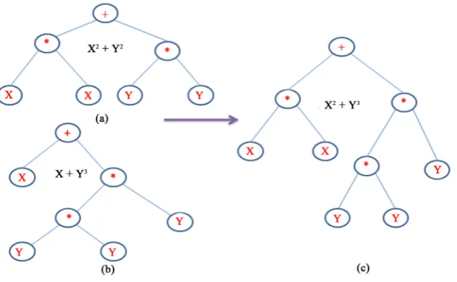
GP is defined as the biologically-inspired evolution of computer programs that solve a predefined task. For this reason, GP is nothing more than a genetic algorithm applied to the problem program evolution. Early GP sys-tems utilized LISP (the original functional programming language, 1958) S-expressions (as shown in Figure 1), but more recently, linear GP systems have been used to evolve instruction sequences to solve user-defined pro-gramming tasks [2].
Since genetic programming manipulates programs by applying genetic operators (reproduction, crossover and mutation), a programming language should permit a computer program to be manipulated as data and the newly created data to be executed as a program. For these reasons, LISP was chosen as the main language for GP.
Evolving complete programs with GP is computationally very expensive, and the results have been limited, but GP does have a place in the evolution of program fragments. For example, the evolution of individual func-tions that have very specific inputs and outputs and whose behavior can be easily defined for fitness evaluation by GP. To evolve a function, the desired output must be easily measurable in order to understand the fitness landscape of the function in order to incrementally evolve it [1]-[7].
Figure 1. Using the crossover operator to create a new S-expression.
3. GP Implementation
The GP uses the same fundamental flow as the traditional genetic algorithm. The population of potential solu-tions is initialized randomly and then their fitness computed (through a simulation of executed instrucsolu-tions with the stack). Selection of members that can propagate into the next generation can then occur through fitness pro-portionate selection. With this method, the higher fit the individual, the higher the probability that they will be selected for recombination in the next generation. Evolutionary algorithms borrow concepts from Darwinian natural selection as a means to evolve solutions to problems, choosing from more fit individuals to propagate to future generations [1]-[7].
The chromosome, or program to be evolved, is made up of genes, or individual instructions. The chromosome can also be of different lengths, assigned at creation, and then inherited during the evolution.
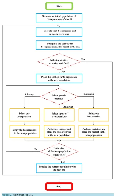
All methods of evolutionary computation (and then GP) work as follows: create a population of individuals, evaluate their fitness, generate a new population by applying genetic operators (Cross-over, mutation and re-production), and repeat this process a number of times as shown in Figure 2.
4. Results and Discussion
We have performed the GP modeling of the inclusive reaction,
p−+Ar, Xe, pb→π±+X
p+pb→charged particles (1) using the experimental data [29]-[32] at 100 and 200 GeV/c and have done so many runs to select the best runs
of the GP program, the first runs are for simulating the rapidity distribution 1 d d
N
N Y of negative pions for
p -Au, Ag, Mg− collisions at 100 GeV/c. They were configured to have the lab momentum
(
PLab)
, massnum-ber (A) and the numnum-ber of particles per unit solid angle (Y) as inputs and the output is the corresponding rapidity
distribution 1 d d
N
N Y
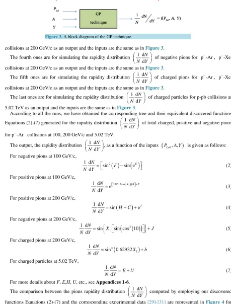
of negative pions at the given momentum as shown in Figure 3.
The second ones are for simulating the rapidity distribution 1 d d
N
N Y
of positive pions for p -Au, Ag, Mg
−
collisions at 100 GeV/c as an output and the inputs are the same as in Figure 3.
The third ones are for simulating the rapidity distribution 1 d d
N
N Y
of positive pions for p -Ar
−
Figure 3. A block diagram of the GP technique.
collisions at 200 GeV/c as an output and the inputs are the same as in Figure 3.
The fourth ones are for simulating the rapidity distribution 1 d d
N
N Y
of negative pions for p -Ar
−
, p -Xe−
collisions at 200 GeV/c as an output and the inputs are the same as in Figure 3.
The fifth ones are for simulating the rapidity distribution 1 d d
N
N Y
of charged pions for p -Ar
−
, p -Xe−
collisions at 200 GeV/c as an output and the inputs are the same as in Figure 3.
The last ones are for simulating the rapidity distribution 1 d d
N
N Y
of charged particles for p-pb collisions at
5.02 TeV as an output and the inputs are the same as in Figure 3.
According to all the runs, we have obtained the corresponding tree and their equivalent discovered functions
Equations (2)-(7) generated for the rapidity distribution 1 d d
N
N Y
of total charged, positive and negative pions
forp -Ar− collisions at 100, 200 GeV/c and 5.02 TeV.
The output, the rapidity distribution 1 d d
N
N Y
, as a function of the inputs
(
PLab, ,A Y)
is given as follows: For negative pions at 100 GeV/c,( )
( )
2 1 d
sin sin e
d
E
N
F
N Y = − (2)
For positive pions at 100 GeV/c,
( )1 0.8613sin 1 d
e d
X R E
N N Y
+
= (3)
For positive pions at 200 GeV/c,
(
)
1 d sin e d J N H CN Y = + + (4)
For negative pions at 200 GeV/c,
( )
(
)
{
2}
1 1 d
sin sin cos 10
d
N
X J
N Y = + (5)
For charged pions at 200 GeV/c,
(
)
4 1 1 d sin 0.62932 d N X bN Y = + (6)
For charged particles at 5.02 TeV,
1 d d
N
E U
N Y = + (7)
For more details about F, E,H, U, etc., see Appendices 1-6.
The comparison between the pions rapidity distribution 1 d d
N
N Y
computed by employing our discovered
collisions at 100 GeV/c, Figure 6 for positive pions for p -Ar− (the GP model cannot describe the data when
the axial value is near 0 because the noisy behavior of data around the axial), p -Xe− collisions at 200 GeV/c.
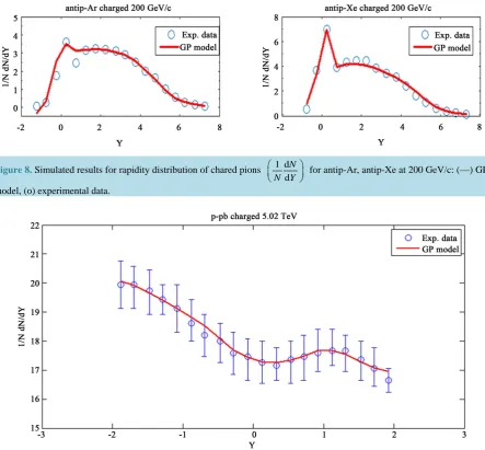
Figure 7 for negative pions for p -Ar− , p -Xe− collisions at 200 GeV/c, Figure 8 for charged pions for
p -Ar− , p -Xe− collisions at 200 GeV/c, Figure 9 for charged particles for p-pb collisions at 5.02 TeV. In order to generate the GP model we have implemented the GP steps (fitness evaluation, reproduction, cros-sover and mutation) that were mentioned in Section 3. Our six discovered functions are generated using the ob-tained control GP parameters, which are shown in Table 1.
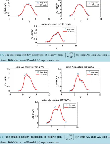
Figure 4. The discovered rapidity distribution of negative pions 1 d d N
N Y
for antip-Au, antip-Ag, antip-Mg
interaction at 100 GeV/c: (—) GP model, (o) experimental data.
Figure 5. The obtained rapidity distribution of positive pions 1 d d N
N Y
for antip-Au, antip-Ag, antip-Mg
[image:6.595.129.512.214.714.2]Figure 6. The discovered rapidity distribution of negative pions 1 d d N
N Y
for antip-Au, antip-Ag, antip-Mg interaction at
100 GeV/c: (—) GP model, (o) experimental data.
Figure 7. GP-simulated for rapidity distribution of negative pions 1 d d N
N Y
for antip-Ar, antip-Xe at 200 GeV/c: (—) GP
[image:7.595.86.539.476.717.2]model, (o) experimental data.
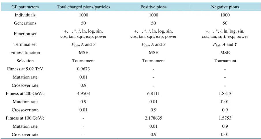
Table 1. Optimal parameters controlling GP program.
GP parameters Total charged pions/particles Positive pions Negative pions
Individuals 1000 1000 1000
Generations 50 50 50
Function set +, −, *, /, ln, log, sin, cos, tan, sqrt, exp, power
+, −, *, /, ln, log, sin, cos, tan, sqrt, exp, power
+, −, *, /, ln, log, sin, cos, tan, sqrt, exp, power
Terminal set PLab, A and Y PLab, A and Y PLab, A and Y
Fitness function MSE MSE MSE
Selection Tournament Tournament Tournament
Fitness at 5.02 TeV 0.9673 - -
Mutation rate 0.01 - -
Crossover rate 0.9 - -
Fitness at 200 GeV/c 4.9503 6.8111 1.8313
Mutation rate 0.9 0.01 0.01
Crossover rate 0.01 0.9 0.9
Fitness at 100 GeV/c ـ 2.178635 1.5753
Mutation rate ـ 0.01 0.9
Figure 8. Simulated results for rapidity distribution of chared pions 1 d d N
N Y
for antip-Ar, antip-Xe at 200 GeV/c: (—) GP
model, (o) experimental data.
Figure 9. The discovered rapidity distribution of charged particles for p-Pb interaction at 5.02 TeV: (—) GP model, (o) experimental data.
The statistical error criterion of mean square error (MSE) was used to measure the deviation between the ex-perimental (actual) and simulated values. The statistical parameter MSE has been used in this work as a per-formance metric [33] to compare the GP simulation with the actual observations (experimental data) and these were evaluated by using Matlab program. The smaller the values of MSE the closer the simulated values to the experimental ones. Our obtained MSE values for the seven discovered functions are given in Table 1, which show also that the performance of the GP model is clearly suitable.
5. Conclusions
GP model has been shown to be a vital method for modeling the h-A interactions. The current article presents an
efficient approach for computing the rapidity distribution 1 d d
N
N Y
of charged, positive and negative pions for
[image:8.595.109.524.279.497.2]References
[1] Jones, M.T. (2008) Artificial Intelligence: A Systems Approach Infinity. Science Press LLC, Hingham.
[2] Banzhaf, W., et al. (1998) Genetic Programming: An Introduction: On the Automatic Evolution of Computer Programs and Its Applications. Morgan Kaufmann, Burlington.
[3] Higuchi, T., Liu, Y. and Yao, X. (2006) Evolvable Hardware. Genetic and Evolutionary Computation.
http://dx.doi.org/10.1007/0-387-31238-2
[4] EvoNews Professor Hans-Paul Schwefel Talks to EvoNews (1999) Available Online.
http://evonet.lri.fr/evoweb/news_events/news_features/
[5] Fogel, L.J., Owens, A.J. and Walsh, M.J. (1966) Artificial Intelligence through Simulated Evolution. Wiley, New York.
[6] Levenick, J.R (1991) Inserting Introns Improves Genetic Algorithm Success Rate: Taking a Cue from Biology. Pro-ceedings on the 4th International Conference on Genetic Algorithms.
[7] Rechenberg I (1965) Cybernetic Solution Path of an Experimental Problem Technical Report Library Translation No. 1122. Royal Aircraft Establishment, Farnborough.
[8] Zheng, S.J., Zhang, N., Xia, Y.J. and Wang, H.T. (2014) Research on Non-Uniform Strain Profile Reconstruction along Fiber Bragg Grating via Genetic Programming Algorithm and Interrelated Experimental Verification. Optics Com- munications, 315, 338-346.
[9] Koza, J.R. (1992) Genetic Programming: On the Programming of Computers by Means of Natural Selection. The MIT Press, Cambridge.
[10] Koza, J.R. (1990) Genetic Programming: A Paradigm for Genetically Breeding Populations of Computer Programs to Solve Problems. Stanford University Computer Science Department Technical Report STAN-CS-90-1314.
[11] Holland, J.H. (1975) Adaptation in Natural and Artificial Systems. University of Michigan Press, Ann Arbor.
[12] Tantawy, M., El-Mashad, M. and El-Bakry, M.Y. (1998) Multiparticle Production Process in High Energy Nucleus- Nucleus Collisions. Indian Journal of Physics, 72A, 73-82.
[13] Moussa, M.A., El-Bakry, M.Y., Radi, A., El-Dahshan, E.-S.A., Habashy, D.M. and Abbas, E.G. (2012) Topological Cross Sections and Multiplicity Distributions for and Interactions at High Energies. International Journal of Scientific and Engineering Research, 3.
[14] Fermi, E. (1950) High Energy Nuclear Events. Progress of Theoretical Physics, 5, 570-583.
http://dx.doi.org/10.1143/ptp/5.4.570
[15] Fermi, E. (1951) Angular Distribution of the Pions Produced in High Energy Nuclear Collisions. Physical Review, 81, 683-687. http://dx.doi.org/10.1103/PhysRev.81.683
[16] Ranft, J. (1970) Secondary Particle Production According to the Thermodynamical Model and New Experimental Data. Physics Letters B, 31, 529-532. http://dx.doi.org/10.1016/0370-2693(70)90082-1
[17] Xu, C., Chao, W.-Q., Meng, T.-C. and Huang, C.-S. (1986) Statistical Approach to Nondiffractive Hadron-Hadron Collisions: Multiplicity Distributions and Correlations in Different Rapidity Intervals. Physical Review D, 33, 1287- 1299. http://dx.doi.org/10.1103/PhysRevD.33.1287
[18] Nambu, Y. (1976) The Confinement of Quarks. Scientific American, 235, 48-61.
http://dx.doi.org/10.1038/scientificamerican1176-48
[19] Gyulassy, M. (1985) Introduction to QCD Thermodynamics and the Quark-Gluon Plasma. Progress in Particle and Nuclear Physics, 15, 403-442. http://dx.doi.org/10.1016/0146-6410(85)90076-6
[20] Kisslinger, L.S. (1985) Nuclear Physics and Quark/Gluon QCD. Nuclear Physics A, 446, 479-488.
http://dx.doi.org/10.1016/0375-9474(85)90624-4
[21] Jacob, M. and Slansky, R. (1972) Nova Model of Inclusive Reactions. Physical Review D, 5, 1847-1870.
http://dx.doi.org/10.1103/PhysRevD.5.1847
[23] Hwa, R.C. (1971) Multiplicity Distribution and Single-Particle Spectrum in the Diffractive Model. Physical Review Letters, 26, 1143-1147. http://dx.doi.org/10.1103/PhysRevLett.26.1143
[24] EL-Bakry, S.Y., El-Dahshan, E.-S. and EL-Bakry, M.Y. (2011) Total Cross Section Prediction of the Collisions of Po-sitrons and Electrons with Alkali Atoms Using Gradient Tree Boosting. Indian Journal of Physics, 85, 1405-1415. [25] El-Bakry, M.Y. (2003) Feed Forward Neural Networks Modeling for K-P Interactions. Chaos, Solitons and Fractals,
18, 995-1000. http://dx.doi.org/10.1016/S0960-0779(03)00068-7
[26] El-Bakry, M.Y. (2004) A Study of K-P Interaction at High Energy Using Adaptive Fuzzy Inference System Interac-tions. International Journal of Modern Physics C, 15, 1013-1020. http://dx.doi.org/10.1142/S0129183104006467
[27] El-Bakry, M.Y., El-Dahshan, E., Radi, A., Tantawy, M. and Moussa, M.A. (2013) A Genetic Programming for Mod-eling Hadron-Nucleus Interactions at 200 GeV/c. International Journal of Scientific and Engineering Research, 4, 7.
[28] Ghosh, D. (1983) International Conference on Cosmic Ray 08.
[29] De Marzo, C., De Palma, M., Distante, A., et al. (1982) Multiparticle Production on Hydrogen, Argon, and Xenon Targets in a Streamer Chamber by 200-GeV/c Proton and Antiproton Beams. Physical Review D, 26, 1019-1035.
http://dx.doi.org/10.1103/PhysRevD.26.1019
[30] Arneodo, M., Arvidson, A., Aubert, J.J., et al. (1987) Comparison of Multiplicity Distributions to the Negative Bi-nomial Distribution in Muon-Proton Scattering. Zeitschrift für Physik C Particles and Fields, 35, 335-345.
http://dx.doi.org/10.1007/BF01570769
[31] Kittle, W. (1973) Combining Inclusive and Exclusive Data Analyses—What Have We Learned So Far? Journal of Physics A: Mathematical, Nuclear and General, 6, 733.
[32] Abelev, B., et al., ALICE Collaboration (2013) Pseudorapidity Density of Charged Particles in p + Pb Collisions at s N N=5.02 TeV. Physical Review Letters, 110, Article ID: 032301. http://dx.doi.org/10.1103/PhysRevLett.110.032301
( )
(
)
10
log cos sin B
D= C+ e , ( )
3 sin 1 0.17 e X D E X
= , 10 1 0.60169
1.2414
X
F= − +
2. Rapidity Distribution of Positive Pions for p−-Au, p−-Ag and p−-Mg Interaction at 100 GeV/c
1
2 1 e 3 970.8738
X
A=X −X − +X − , B=X2−0.12013−tan
( )
A ,(
)
( )3
( )
sin
3
10 X cos
C= B − X ,
(
)
2
cos 0.187454
D= +C , E=sin2
(
0.550985X1)
−D,( )
(
)
(
( )
( )
)
(
3)
10 3 3
cos log tan tan eX cos
F= X + − X ,
( )
3 3 2(
1 2)
tan 10
G= X +X X − X + X , H =sin
( )
G 10 F,3 2.91765 10 I X − = ,
(
3)
3
10 X I 0.82908 H J
X
− +
= ,
(
( )
)
( )
( )
310 3 3
log tan cos tan eX
K= X + X − ,
3
2 3 2 10
X
L=X +X X − ,
( )3 sin 1 2 10 0.82908 X X M X + = −
, 3
3.64929 sin 10 N X − = ,
(
3)
cos sin 10 N
O= X +m, sin cos
( )
I 0.8298 O K P J L = + − ,(
)
( )
3 1sin 0.176 cos
Q= X − P , R=tan e
( )
Q3. Rapidity Distribution of Positive Pions for p−-Xe and p−-Ar Interaction at 200 GeV/c
[
1]
1.228815 0.831998 A X = , ( ) sin 1 e 0.724939 A B X
= , 1cos 0.984928 sin e
(
sin( ))
B
C=X ,
( )
(
)
( )
1 10 1 10 cos sin56.2934 log X D X = − ,
( )
(
)
( )
21 10 1
sin cos 10 log
E= X − D− X ,
( )
( )
sin 0.984928sin e AG= , H =0.984928sin2
(
G+E)
, I =0.942092 cos( )
X2 ,(
)
1 e 0.20605 I J X =
4. Rapidity Distribution of Negative Pions for p−-Ar and p−-Xe Interaction at 200 GeV/c
( )
1 cos 2 3 10 1 10e
X X
A=X X + , 1
1
10 sin 0.995888
0.39473
X
B= X +
(
e10.66922)
2( )
3
e X cos
C= + − X ,
2
1
10 0.39473
eX
X
D=
,
3
X
E C B
D = − ,
( )
2 1 3 10 cos sin 0.39473 XG= F −X
,
( )
1 10 3 10 log 0.39473 XH = G − X
,
( )2 sin
1 sin e X
I = X ,
( )3
5. Rapidity Distribution of Charged Pions for p−-Xe and p−-Ar Interaction at 200 GeV/c
(
)
30.13958 1 1 2 sin 0.9331 X X
A= X X −
, 7.6003 2 1 10 log 0.533419 X A X B − =
, C=sin2
(
0.62932X1)
+B,(
)
2
1
sin sin 0.62932 0.37885
D= X − ,
2 2 0.13958 1 2 1 X X X E X X + = −
, 2
(
)
1 10
sin 0.62932 log E
F X D = + ,
( )
{
}
0.13958sin C 1
G= F − ,
(
0.88504)
0.760032 2
H = X +X ,
2 1 0.533419 H X G X I − = ,
(
)
( )
2 1 10sin sin 0.62932 log
J= X + I , K =sin 0.62932
(
X1)
−tan sin( )
X2 ,( )
10.841471cos K
L= X ,
( )
0.13958 2
3
3 2
sin cos cos
0.88504
X
M L X
X = − + , 2 2 1 1 X X X N M X + = − ,
(
)
(
)
2 1 10sin sin 0.62932 log 0.41797
N O X = + ,
(
)
( )
2 1 10sin sin 0.62932 log
P= X + O ,
(
)
30.13958 1 2 1 sin 0.9331 X X
Q= X X −
,
( )
{
}
0.760030.88504
3 2
sin
R= X +X ,
0.13958 2 1 10
log
0.533419
R X X
S= Q −
,
(
)
2
1 sin 0.62932
T = X +S,
( )
10 3 3 2 3 log 0.010309 e
X X X X
U
+ +
= , cos
( )
eU
T
V = P ,
( )
1 3 2 3 sin 10 e cos 0.04686 X X W X = + − ,
{
(
)
3}
0.139581 3
sin X 1
X = X X − ,
( )
{
3 0.88504}
0.760031 sin 2 2
X
Y= X − X +X ,
(
1)
sin( )
Y
X
Z= VW−X ,
(
2 1)
21
X X X
a Z J
X + = − ,
(
)
( )
2 1 10sin 0.62932 log
b= X + a
6. Rapidity Distribution of Charged Particles for p-pb Interaction at 5.02 TeV
(
) (
10 1)
0.05142
0.949882
x
A= − − , B= −9.64173 cos
( )
X1 ,(
0.786251)
B
C= , D= +C log2sin 10
( )
−log 102( )
,( )
2
log e
22026.47 D
E= ,
( )
110 1
1
0.97842
log 10 log eX
F X
X
= +
( )
( )
1 10.259004
cos 10 log
N X
X
= − + , O=1.557408N , P=1.557408
(
O− m)
, Q=(
e0.671654 tan( )X1X12)
,( ) 2 1 1
tan
e X X Q
R=
,
1
10
cos e
1.071185 X
S R
= − , T =1.557408 cos
( )
x1 −S,( )
( )
( )
10 1 log
2 2
e
log sin 10 log 10
X T
U
−
=
−
,
( )1
9.642 cosX
V =U− , W=log2
{
log2log2(
log10(
0.98407− −x1 2.142536)
)
}
−3.321928+V,8.036777 0.80812
X
x
= +
, Y =1.557408 cos
( )
x1 − log( )
x1 +1,( )
( )
10 1 log
1 e cos
0.70831
X Y
Z x W
−
= −
,
( )
1( )
11
0.259004
cos log
a X X
X
= − + ,
0.8901
1 10 log
tan e X
b a
=
, c= −b log
( )
X1 +Z ,( )
10 1 log
0.30103 tan e
X
d=c
,
( )
(
log10)
log e c P
e= − F − , f =ee 10( −X1)
where, X1 is the number of particles per unit solid angle (Y), X2, lab momentum