Nonlinear dynamics in a model of
financial development with a risk
premium
Gomes, Orlando
Escola Superior de Comunicação Social - Instituto Politécnico de
Lisboa
February 2007
Online at
https://mpra.ub.uni-muenchen.de/2887/
Nonlinear Dynamics in a Model of Financial Development
with a Risk Premium
Orlando Gomes
∗Escola Superior de Comunicação Social [Instituto Politécnico de Lisboa] and Unidade de Investigação em Desenvolvimento Empresarial [UNIDE/ISCTE].
- February, 2007 -
Abstract: The relation between the degree of financial development of an economy (measured by the extent in which constraints to credit exist) and fluctuations affecting the trend of economic growth, is a relevant theme of discussion in macroeconomics. Some of the literature on this field argues that the cyclical behaviour is generated endogenously, under the model’s assumptions, for specific levels of credit availability. Following this line of reasoning, the paper develops a theoretical framework that places a risk premium over the international interest rate as the centre piece of the explanation for the occurrence of endogenous business cycles, under particular levels of financial development. The risk premium penalizes the borrowing capacity of the less wealth endowed countries. The analysis explores both local and global dynamics.
Keywords: Financial development, Credit constraints, Risk premia, Endogenous business cycles, Nonlinear dynamics, Chaos
JEL classification: O16, E32, C61.
∗ Orlando Gomes; address: Escola Superior de Comunicação Social, Campus de Benfica do IPL,
1549-014 Lisbon, Portugal. Phone number: + 351 93 342 09 15; fax: + 351 217 162 540. E-mail:
1. Introduction
From an empirical point of view, it is well accepted that the level of financial
development is strongly correlated with economic growth, at least in the short run. This
result is highlighted, for instance, by Levine (1997, 2005), Demirguç-Kunt and Levine
(2001) and Christopoulos and Tsionas (2004); these last authors present evidence that
allow to conclude that the causality runs from finance to growth, and not the other way
around. This result seems logical: developed financial markets, in which barriers to
credit are not too relevant, contribute to an efficient allocation of productive inputs
across economic agents and also in a temporal perspective, allowing for a potentially
higher level of generated income.
This simple and intuitive result is relevant when trying to establish a link between
the long term growth trend and short run fluctuations. Somehow surprisingly, theories
on business cycles and on economic growth have evolved under separate paradigms
that rarely intersect each other. Aghion, Angeletos, Banerjee and Manova (2005) stress
this odd fact, by recognizing that the modern theory of cycles gives relevance to the
degree of financial development as a source of propagation of productivity shocks, but
in business cycles analysis these disturbances frequently arise as exogenous; in the
opposite field, the modern growth theory emphasizes the central role of productivity
and often considers it as the outcome of an endogenous production process, in order to
explain growth trends, but it neglects any mechanism of propagation that eventually
generates short run fluctuations.
This paper intends to contribute to the literature on the integrated approach to
growth and cycles in environments where the degree of financial development may
vary. Such literature has benefited from important contributions, starting with the work
of Bernanke and Gertler (1989), King and Levine (1993) and Kyotaki and Moore
(1997).
Recently, the subject has gained a new impulse with the work of Philippe Aghion
and his co-authors. Aghion, Banerjee and Piketty (1999) presented the benchmark
model; in this model, the macroeconomic setup is characterized by the existence of an
agency problem that limits the access of firms to credit, an element that is modelled by
assuming a credit multiplier as the one initially proposed by Bernanke and Gertler
(1989). The capital market imperfections generate endogenous fluctuations that persist
rate) will exhibit cycles that are well explained from an economic intuition point of
view: there is a multiplier effect of investment that conflicts with increasing interest
rates that higher investment levels produce, that is, the tension of two forces that push
investment in opposite directions generates and allows to sustain endogenous cycles
over time.
The previous work has been extended by Aghion, Baccheta and Banerjee (2004),
who study the effects of financial development over small open economies, and
conclude that unstable dynamics (in the case, just period two cycles) arise for
intermediate levels of financial development, while stability prevails in economies that
have credit systems that are either underdeveloped or significantly developed.
In Aghion, Baccheta and Banerjee (2000, 2001), a similar type of analysis is
undertaken, but in these studies the focus lies in monetary economies characterized by
the presence of nominal price rigidities. The main conclusions are: (i) in credit
constrained economies in which debt is issued both in domestic and foreign currencies,
currency crises are likely to arise; (ii) currency crises generated by the interplay
between credit constraints and price sluggishness are associated with the presence of
multiple equilibria.
Finally, the work by Aghion, Howitt and Mayer-Foulkes (2005) establishes the
bridge between financial development and growth convergence. Their model proposes
an explanation of growth where the growth rate of an economy with a high level of
financial development will converge to the rate of growth of the world technology
frontier, while all the other economies will systematically grow at a lower rate.
The framework that we propose in the following sections concerns to an
endogenous growth setup. This has been the main theoretical structure in which the
problem under discussion has been addressed. This is the case of the previously
discussed references, as well as of other studies, like Amable, Chatelain and Ralf
(2004), who analyze how credit rationing affects endogenous growth when debt is
related to the firm’s internal net worth taken as collateral, Blackburn and Hung (1998)
and Morales (2003) who concentrate in growth models based on innovation to study the
relationship between finance and growth, and also Harrison, Sussman and Zeira (1999)
and Khan (2001) who integrate financial intermediation and growth under an AK
growth model. The model that we intend to analyze takes as well an AK production
function.
Besides the literature on the link between financial development and endogenous
initially developed by Benhabib and Day (1981), Day (1982) and Grandmont (1985),
among many others, and that was recovered later essentially by two strands: first, the
one that searches for non linear dynamics in optimal growth models under competitive
markets. Here, we can include Nishimura, Sorger and Yano (1994), Boldrin,
Nishimura, Shigoka and Yano (2001), and related literature. These authors search for
extreme conditions under which endogenous fluctuations arise in competitive
frameworks (e.g., too low discount factors or peculiar types of production functions).
Second, it is relevant to mention the work that has adapted the Real Business
Cycle model to a completely deterministic setup able to produce long run business
cycles. This work was initiated by Christiano and Harrison (1999), and further
developed by Schmitt-Grohé (2000) and Guo and Lansing (2002), among others. These
endogenous growth models take the structure of the Real Business Cycle models,
namely, a setup where the representative agent has two types of choices to make
(between consumption and savings, on one hand, and between leisure and work time,
on the other hand), and add to it a production function exhibiting increasing returns to
scale (that can result, for instance, from a positive externality on the production of final
goods). This framework, that can be contested by the evidence that only too high
externality levels are able to produce endogenous cycles, is able to generate cycles of
various periodicities including chaotic motion. See Gomes (2006) for a survey on
macroeconomic models capable of reproducing cycles as a result just of the non linear
relation between economic aggregates.
The model to be presented and discussed is essentially based on the theoretical
structure developed by Caballé, Jarque and Michetti (2006) [hereafter CJM]. These
authors propose to present a model of financial development pointing to a set of results
close to the ones by Aghion, Baccheta and Banerjee (2004), that is, growth related
instability eventually arises for intermediate levels of financial development and
stability prevails for both low and high levels of credit worthiness. Nevertheless, the
type of fluctuations found in the CJM model is much more comprehensive, in the sense
that it is not limited to period two cycles, but higher order cycles and complete
a-periodicity (including chaos) are obtainable.
The framework to develop below is based on the structure of the CJM model,
with two important differences: first, we consider a unique input that is internationally
available (the CJM model takes a second production factor, which is country specific);
second, besides a constraint on credit, we include a second limitation that firms in less
premium is charged over countries that are less endowed in terms of accumulated
wealth. This alternative structure is able to generate, for specific values of some
meaningful parameters, endogenous cycles of various periodicities, including chaotic
motion.
The model is analyzed both in terms of local and global dynamics. Locally, one
identifies the points where bifurcations separate regions of stability (or saddle-path
stability) from regions of instability; globally, one confirms that stability truly prevails
on the areas identified locally as such, while in the locally unstable areas, we find a
region of cyclical behaviour before instability becomes dominant (here, we identify
instability with the notion of variables diverging to infinity).
Synthesizing, the paper takes the a model of financial development and growth,
simplifies its structure in terms of production conditions (a one input AK production
function is taken), introduces a risk premium over the interest rate, and it proposes to
analyze this alternative framework about finance and growth. As in the CJM study,
completely a-periodic cycles are generated.
The remainder of the paper is organized as follows. Section 2 presents the
structure of the model. Section 3 studies local dynamics and section 4 global dynamics.
Section 5 presents an additional feature by introducing endogenous technical progress.
Finally, conclusions are left to section 6.
2. The Model
We consider a small open economy where a large number of households and firms
interact. In this economy, population does not grow and, hence, all aggregate variables
may, indistinctively, be considered level or per capital variables. We assume that
households consume a constant share of the economy’s income, that is, we take c∈(0,1) as the marginal propensity to consume. Firms generate wealth through the production of
goods given the resources available for investment.
Basically, we will work with an endogenous growth setup, since the aggregate
production function to consider is of the AK type, i.e., yt=Akt, with A>0 an index of
technological capabilities and yt and kt the levels of output and physical capital in a
given time moment t. Assuming that capital fully depreciates after one period, there is a coincidence between investment and the stock of capital, it=kt, and thus output grows
Firms can borrow funds in the domestic financial markets in order to finance their
productive projects. The international nominal rate of interest is r>0, but firms have access to loans at this rate only if the level of accumulated wealth of the economy is not
below a given threshold value (wt*) imposed by monetary authorities. When the
economy’s level of wealth, wt, is below the benchmark level, financial markets perceive
a risk associated to loans and therefore they will charge a higher interest, which is as
much higher as the larger is the difference between wt and wt*. Consequently, for low
levels of development (relatively low levels of accumulated wealth), the interest rate
becomes a decreasing function of wealth. Formally, the domestic interest rate on
productive loans will be
≥
<
⋅ =
+
*
* *
1
if
if
t t
t t t
t t
w w r
w w w
w f r
r (1)
In (1), we introduce a time lag by assuming that today’s wealth levels will be
reflected on tomorrow’s interest rate. Function f is continuous and differentiable, with
fw<0, lim* *=1
→
t t w
w w
w
f and f(0)→+∞, i.e., an infinite interest rate is hypothetically
applied over loans when the economy is hypothetically endowed with no resources.
Furthermore, we assume that if =
ξ
*
t t
w w
f , with
ξ
some positive constant, we cancompute an inverse function f-1, such that wt = f 1( )⋅wt*
− ξ
; the following properties
should apply: fξ−1 <0 and f−1
( )
1 =1.Function f reflects the risk premium on loans. Possibilities of profitable investment
require considering that the marginal productivity of capital exceeds the lowest possible
interest rate, i.e., A>r.
Besides the imposition of a risk premium, the financial sector will be
characterized as well by placing quantitative constraints on credit. These may reflect,
for instance, inefficiencies arising from information asymmetries. The level of wealth
serves as collateral to loans, and firms may borrow at most µwt, with µ>0 a credit
multiplier that is supposed to translate the level of financial development of the national
premium that affects the price of credit; second, a level or quantitative boundary that
imposes a ceiling on the availability of credit.
Wealth dynamics will be given by a simple rule. We just consider that next
period’s level of wealth corresponds to the non consumed income, with income given
by output less debt payment. Letting bt be the amount of financial resources that are
borrowed by firms in moment t, we have
) (
) 1 (
1 t t t
t c y r b
w+ = − ⋅ − ⋅ , w0 given. (2)
In difference equation (2), the output level may be replaced by an expression
reflecting the level of investment. Noticing that the economy will invest, on aggregate,
the level of available wealth plus the borrowed resources, then it=wt+bt, and therefore
output comes yt = A⋅(wt +bt). Equation (2) is, thus, equivalent to
[
t t t]
t c Aw A r b
w+1 =(1− )⋅ +( − )⋅ .
Two cases are clearly distinct, in what concerns firms’ behaviour. First, if A≥rt
then it is profitable to invest in production the largest amount that it is possible to
borrow. With a marginal productivity above the financial return, firms choose bt=µwt,
and thus equation (2) becomes
[
t]
tt c A r w
w+1 =(1− )⋅ ⋅(1+µ)−µ⋅ ⋅ , (A≥rt). (3)
Second, when A<rt firms borrow only until the point where the productive
marginal return is equal to the interest rate, that is, yt −rt ⋅bt =rt ⋅wt. Therefore,
t t
t c r w
w+1 =(1− )⋅ ⋅ , (A<rt). (4)
It is important to associate the previous wealth expressions with our interest
condition (1). Observe that under A≥rt we have
r A w
w f
t t ≥
− −
* 1
1 , which is equivalent to
* 1 1
1 −
−
− ⋅
≥ t
t w
r A f
w . Likewise, A<rt implies the relation −1 −1 ⋅ *−1
< t
t w
r A f
w . Remind
particularly, it is true that 1 <1 − r A
f , and this condition allows to distinguish among
three different states of the assumed economy, according to the following diagram:
The previous scheme reveals that the wealth dynamics equation is a piecewise
function with three segments, as follows
[
]
≥ ⋅ ⋅ − + ⋅ ⋅ − < ≤ ⋅ ⋅ ⋅ ⋅ − + ⋅ ⋅ − ⋅ < ⋅ ⋅ ⋅ − = − − − − − − − − − − − − − + * 1 1 * 1 1 * 1 1 * 1 1 * 1 1 1 * 1 1 1 if ) 1 ( ) 1 ( if ) 1 ( ) 1 ( if ) 1 ( t t t t t t t t t t t t t t t w w w r A c w w w r A f w w w f r A c w r A f w w w w f r c wµ
µ
µ
µ
(5)The assumption of an AK production function implies that our setup is an
endogenous growth framework, in the sense that all the mentioned aggregates (yt, kt, it,
wt) grow in the steady state at a positive and constant rate. Let this rate be
γ
>0 andassume that the benchmark level of wealth, wt*, represents a trend of accumulated
wealth, such that it grows at rate
γ
for all t. We define constant wt tw ) 1 ( ˆ * *
γ
+≡ and
variable t t t w w ) 1 ( ˆ
γ
+≡ . System (5) is now rewritten for the detrended variable:
[
]
≥ ⋅ ⋅ − + ⋅ ⋅ + − < ≤ ⋅ ⋅ ⋅ ⋅ − + ⋅ ⋅ + − ⋅ < ⋅ ⋅ ⋅ + − = − − − − − − − + * 1 * 1 * 1 * 1 * 1 1 * 1 1 ˆ ˆ if ˆ ) 1 ( 1 1 ˆ ˆ ˆ if ˆ ˆ ˆ ) 1 ( 1 1 ˆ ˆ if ˆ ˆ ˆ 1 1 ˆ w w w r A c w w w r A f w w w f r A c w r A f w w w w f r c w t t t t t t t t tµ
µ
γ
µ
µ
γ
γ
(6) * 1 1 −− ≥ t
t w
w *
1 1 −
− < t
t w
w
A≥rt
The dynamic analysis of system (6) requires transforming the one equation / two
time lags expression into a two equations / one time lag system. This may be done by
defining variables w~t ≡wˆt −w and ~zt ≡wˆt−1−w, with w an equilibrium point of
system (6). The system that will be subject to analysis is, thus, the one in expression (7).
[
]
= − ≥ − + ⋅ ⋅ − + ⋅ ⋅ + − − < ≤ − ⋅ − + ⋅ + ⋅ ⋅ − + ⋅ ⋅ + − − ⋅ < − + ⋅ + ⋅ ⋅ + − = + − − + t t t t t t t t t t t w z w w z w w w r A c w w z w w r A f w w w w w z f r A c w w r A f z w w w w w z f r c w ~ ~ ˆ ~ if ) ˆ ( ) 1 ( 1 1 ˆ ~ ˆ if ) ˆ ( ˆ ~ ) 1 ( 1 1 ˆ ~ if ) ˆ ( ˆ ~ 1 1 ˆ 1 * * * 1 * * 1 * 1 µ µ γ µ µ γ γ (7)Note that the steady state values of variables w~ and t z~ are, both, zero. t
The first step to analyze (7) consists in determining the steady state. Two steady
state points are feasible. The first is valid for 1 wˆ*
r A f
w ⋅
< − ; the second for
* 1 ˆ w r A f
w ⋅
≥ − . They are, respectively, 1 *
1 ˆ ) 1 ( 1 w r c f
w ⋅
⋅ − +
= −
γ
and* 1 2 ˆ 1 1 ) 1 ( w r c A f w ⋅ ⋅ − + − + ⋅ = −
µ
γ
µ
.Two steady state points exist under the assumption that f−1
( )
⋅ is a constant value.The following condition is essential to guarantee a positive long run level of wealth:
c A − + > + ⋅ 1 1 ) 1
( µ γ .
3. The Analysis of Local Bifurcations
Because system (7) has two equilibrium points, local dynamics must be dissected
in the vicinity of each one of these points. Let us start by taking w1. The equilibrium point exists for the first equation of the system. Linearizing the system in the vicinity of
⋅ ⋅ ⋅ ⋅ + − = + + t t z t t z w w f r c z w ~ ~ 0 1 1 1 1 ~ ~ 1 1 1 γ (8)
In (8), fz represents the derivative of function f in order to ~ . The sign of zt fz determines the type of dynamics underlying the system. Because ~ is just a linear zt
transformation of wˆ , we must have t fz<0. The dynamic behaviour is characterized in
proposition 1.
Proposition 1. Local dynamics in the vicinity of the first equilibrium point, w1, are
expressed on the following conditions:
i) If 1
1 1
1 >−
⋅ ⋅ ⋅ + − w f r c z
γ , then the system is stable in the neighbourhood of w1;
ii) If 1
1 1
1 <−
⋅ ⋅ ⋅ + − w f r c z
γ , then the system is unstable in the neighbourhood of
1
w ;
iii) If 1
1 1
1 =−
⋅ ⋅ ⋅ + − w f r c z
γ , then a Neimark-Sacker bifurcation occurs.
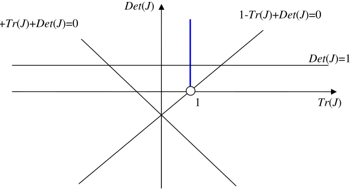
Proof: The trace and the determinant of the Jacobian matrix in (8) are, respectively, Tr(J)=1 and Det(J)= 0
1 1 1 > ⋅ ⋅ ⋅ + −
− c r fz w
γ . Conditions for stability are
1-Tr(J)+Det(J)>0 ⇒ 0 1 1 1 > ⋅ ⋅ ⋅ + −
− c r fz w
γ , which is an universal condition;
1+Tr(J)+Det(J)>0 ⇒ 0 1
1
2 ⋅ ⋅ ⋅ 1 >
+ −
− c r fz w
γ , which is also an universal condition; and
1-Det(J)>0 ⇒ 1 1
1
1 >−
⋅ ⋅ ⋅ + − w f r c z
γ , a condition that applies only for certain
combinations of parameter values. Thus, stability can only break down in the
circumstance in which the eigenvalues of J become a pair of complex conjugate
eigenvalues, i.e., when Det(J)=1, or, yet, a Neimark-Sacker bifurcation occurs.
Condition Det(J)>1 implies instability. Figure 1 depicts graphically this stability result.
Consider now w2. This equilibrium relates to the second equation of (7). Once again, we linearize the system, to obtain
⋅ ⋅ ⋅ ⋅ ⋅ + − − = + + t t z t t z w w f r c z w ~ ~ 0 1 1 1 1 ~ ~ 2 1 1 µ γ (9)
Proposition 2. In the vicinity of w2, the dynamics of the financial model are given
by the following conditions:
i) If 2
1 1
2 >−
⋅ ⋅ ⋅ ⋅ + − w f r c z µ
γ , then the system is saddle-path stable in the
neighbourhood of w2;
ii) If 2
1 1
2 <−
⋅ ⋅ ⋅ ⋅ + − w f r c z µ
γ , then the system is unstable in the neighbourhood of
2
w ;
iii) If 2
1 1
2 =−
⋅ ⋅ ⋅ ⋅ + − w f r c z µ
γ , then a bifurcation occurs.
Proof: Once again, we look at conditions 1-Tr(J)+Det(J)>0, 1+Tr(J)+Det(J)>0 and 1-Det(J)>0 to characterize stability. The first is never satisfied, thus stability (stable
node or stable focus) cannot hold; because Det(J)<0, the third condition is always
verified. Thus, it is through the analysis of the sign of 1+Tr(J)+Det(J) that we can
distinguish between stability outcomes. When Det(J)<-2, we will have a saddle-path
stable equilibrium (one of the eigenvalues of the Jacobian lies inside the unit circle,
while the other does not); Det(J)>-2 implies instability (both eigenvalues outside the
unit circle). A bifurcation separates the two referred regions, for Det(J)=-2. The three
previous conditions are equivalent to the ones in the proposition.
Relatively to the bifurcation observe that for the presented determinant value, the
two eigenvalues of J are -1 and 2. Note that this cannot be considered a flip bifurcation,
because although this kind of bifurcation implies that one of the eigenvalues must be
equal to -1, it also requires that Tr(J)∈(-2,0) and Det(J)∈(-1,1), which is not the case.
Graphically, we have
Specific f function. Consider now the following particular function f: θ − = * * t t t t w w w w
f , θ>0. This function obeys to the properties previously postulated.
With a particular functional form, one is able to present explicit expressions for the
steady states. They are
* / 1 1 ˆ 1 ) 1 ( w r c
w ⋅
+ ⋅ − = θ
γ and *
/ 1 2 ˆ 1 1 ) 1 ( w c A r w ⋅ − + − + ⋅ ⋅ = θ γ µ µ .
According to system (7), we must have w2 >w1, which is equivalent, under the specific case in consideration, to
c A − + < 1 1 γ
. Combining this relation with the constraint
that allows for a positive w2, we can present the following boundary values for the economy’s growth rate:
γ
∈(
A⋅(1−c)−1;(1+µ
)⋅A⋅(1−c)−1)
. The growth rate is bounded given the level of technology, the marginal propensity to consume and thelevel of financial development. This last parameter is particularly relevant, because it
establishes a relation between constraints on credit and growth: the lower are the
constraints, the higher is the potential pace of growth.
Local dynamics can be addressed under the specific risk premium function. The
Jacobian matrices are, for each one of the equilibrium points:
− = 0 1 1 1 θ
J for w1;
− + − ⋅ + ⋅ ⋅ = 0 1 1 1 1 ) 1 ( 1 2
γ
µ
θ
A cJ for w2.
Matrices J1 and J2 are particular cases of the matrices in (8) and (9). In the first
case, a unique bifurcation parameter exists:
θ
<1 implies stability andθ
>1 instability. ANeimark-Sacker bifurcation occurs at
θ
=1. For w2, the combination of parameters separating the region of saddle-path stability from instability isθ
θ
γ
µ
2 1 1 ) 1 ( = + + − ⋅ + ⋅ cA ; we conclude that the higher the degree of financial
development, the more likely will be the situation in which the system falls into the
The analysis of global dynamics will allow to clarify the apparent paradox that the
previous arguments enclose: first, we have stated that a higher degree of financial
development allows for a potentially higher growth rate, which seems an intuitive
result; second, high values of parameter
µ
are associated with instability (this resultclearly arises in the global analysis of the section that follows). This result may be
justified under the idea that a too high level of
µ
means too few constraints on credit, ortoo low collateral requirements on loans. This, in turn, can increase the risk of failure in
paying the loans by the borrowers, what can lead to situations of strong decline in the
confidence underlying the financial system that may culminate in financial crises.
Instability for high values of
µ
can therefore be associated to credit availability that isnot constrained by any precautionary measures.
4. Global Dynamics
The study of global dynamics requires the consideration of a specific form of the
system (we consider a same f function as in the final part of the previous section) and to
assume some benchmark values for parameters. The following are chosen as reasonable
values: c=0.75,
γ
=0.04 and r=0.03; we take as well the indexes ˆ* =1w and A=3. The
remaining two parameters,
θ
andµ
, will assume several different values in the analysis.Note that although system (7) may be analyzed in terms of global dynamics, it is a
different system for different equilibrium values. Hence, we should study dynamics
taking, alternatively, w1 and w2. Let us start by considering w1. In this case, local dynamics has pointed to a Neimark-Sacker bifurcation occurring at
θ
=1. For values ofθ
below one, stability prevails (in this case, the global dynamics result is coincidental with
the result found locally), while for values of
θ
above 1 a region of endogenous cycleswill arise before instability sets in.1
One of the values of
θ
for which cycles are present isθ
=1.3. For this value, wedraw a bifurcation diagram concerning parameter
µ
. One observes that fluctuationsindeed prevail for a given set of values of the credit multiplier. Note that
µ
is bounded
1
from above, given condition
c A
− + > + ⋅
1 1 ) 1
(
µ
γ
. Figure 3 displays the bifurcationdiagram.2
- Figure 3 here -
Recall that w~ is a variable that is modified twice. First, it was detrended and then t
it was normalized to a zero steady state. The original variable has a positive detrended
equilibrium value and follows an upward sloping trend. The modified variable follows,
for a specific value of
µ
for which fluctuations are evident (µ
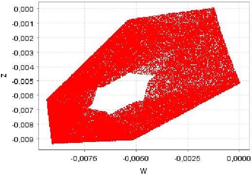
=1.5), the time pathdisplayed in figure 4. Figure 5 presents, for the same value of
µ
, the long term attractingset of the relation between w~ and t z~ . t
- Figures 4 and 5 here -
The presence of chaotic motion is well demonstrated through the graphical
examples, but we can reemphasize the idea by computing Lyapunov characteristic
exponents (LCEs). These are a measure of chaos and they indicate the presence of this
type of dynamic behaviour if, in a two dimensional system as the one we consider, at
least one of the two LCEs is positive. LCEs evaluate the exponential divergence of
nearby orbits, that is, they search for sensitive dependence on initial conditions, a
property that is accepted to characterize the presence of chaotic motion. Sensitive
dependence basically means that if a same deterministic system initialized in two
distinct points (even though these may be located very close to each other) it produces
long term time series that have no identifiable common features.
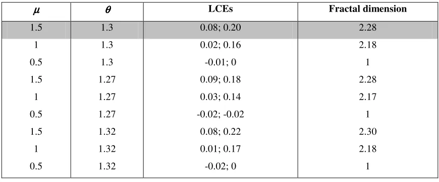
Table 1 presents the computation of LCEs and the fractal dimension of the
attractor, for various values of parameters
θ
andµ
.3 The fractal dimension of theattractor is given by the formula
1 2
1
λ
λ
+ =D , according to the definition by Kaplan and
Yorke (1979), where
λ
1 is the negative LCE andλ
2 the positive one. If both LCEs are
2
All the figures concerning global dynamics presented in this paper are drawn using IDMC software (interactive Dynamical Model Calculator). This is a free software program available at
www.dss.uniud.it/nonlinear, and copyright of Marji Lines and Alfredo Medio.
3
positive, a circumstance that eventually occurs and that is generally designated by hyper
chaos, then the attractor dimension is D=2+
λ
1+λ
2, with bothλ
1 andλ
2 above zero.4Evidently, the fractal dimension can only be computed for chaotic systems;
otherwise, the dimension of the attractor in an order 2 system is equal to 1, that is, the
fractal dimension has correspondence on the Euclidean dimension. The non integer
dimension that one finds when chaos exists can be thought of as a measure of the degree
of chaos. We will have D>1, and the higher is D, the stronger is the chaotic nature of
the system, in the sense that the divergence of nearby orbits is more intense.
µµµµ θθθθ LCEs Fractal dimension
1.5 1.3 0.08; 0.20 2.28
1 0.5 1.5 1 0.5 1.5 1 0.5
1.3 1.3 1.27 1.27 1.27 1.32 1.32 1.32
0.02; 0.16 -0.01; 0 0.09; 0.18 0.03; 0.14 -0.02; -0.02
0.08; 0.22 0.01; 0.17 -0.02; 0
[image:16.595.78.513.251.432.2]2.18 1 2.28 2.17 1 2.30 2.18 1
Table 1 – LCEs and fractal dimensions for system (7), with w = w1.
In table 1, we consider three possible values for
µ
andθ
. The dynamics are verysensitive to the value of
θ
; and therefore we consider three values of this parameter thatare close together and that involve the presence of chaotic motion. We observe that for
µ
=0.5, chaos is ruled out, independently of the value ofθ
, whileµ
=1 andµ
=1.5 correspond to cases of hyper chaos for the selected values of the parameterθ
. In thesecases we compute a fractal dimension higher than 2.
Consider now the alternative case, where w =w2. As one has observed through the local analysis, the system now undergoes a different type of bifurcation. Thus, we
will certainly obtain distinct dynamic results. In this case, we consider
θ
=1.1, a valuethat leads us directly to the region of endogenous fluctuations. Figure 6 respects to the
bifurcation diagram regarding the credit boundary variable,
4
- Figure 6 here -
Once more, cycles of no identifiable periodicity are observed for a given interval
of values of the credit parameter. The wealth variable is subject to business cycles, as it
can be confirmed by looking at the diagrams in figures 7 and 8 (observe the similarity
between the strange attractors in figures 5 and 8).
- Figures 7 and 8 here -
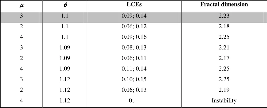
[image:17.595.79.512.317.493.2]Chaotic motion is confirmed through the computation of LCEs and presentation of
table 2, which has a same type of contents as table 1.
µµµµ θθθθ LCEs Fractal dimension
3 1.1 0.09; 0.14 2.23
2 4 3 2 4 3 2 4
1.1 1.1 1.09 1.09 1.09 1.12 1.12 1.12
0.06; 0.12 0.09; 0.16 0.08; 0.13 0.06; 0.11 0.11; 0.14 0.10; 0.15 0.06; 0.13
0; --
2.18 2.25 2.21 2.17 2.25 2.25 2.19 Instability
Table 2 – LCEs and fractal dimensions for system (7), with w = w2.
The analysis of table 2 indicates the presence of different ‘degrees’ of chaos for
several values of the parameters, with
θ
above but close to unity. Note that cases ofhyper chaos, that is, attractors with dimensions higher than two are, once again,
observed.
As regarded, assuming one or the other equilibrium value, implies getting
different dynamic results, but in both cases we find regions of chaotic motion for some
values of the level of financial development, meaning that endogenous business cycles
may arise as the result of a combination of quantitative constraints on credit and a risk
5. An Extension: Endogenous Technological Progress
The model in the previous sections may be extended in several directions. In what
follows, we consider that the generation of technology is endogenous, through two
assumptions that do not change significantly the qualitative nature of the model, but that
allow to find additional results concerning non linear long run behaviour. The two
assumptions are: (i) technology is the only input in the production of additional
technology; (ii) decreasing marginal returns are assumed in order to obtain a stable
equilibrium point.
The dynamic behaviour of the technology variable is given by
) (
1 t
t g A
A+ = , with A0 given, g>0, g’>0 and g’’<0. (10)
Endogenous technology growth implies two changes in our framework:
equilibrium values w1 and w2 will depend on the steady state value of A, and the conditions that characterize the different states (i.e., At<rt and At≥rt) are now dependent
on the evolution of the technology variable.
In what concerns local dynamics, we do not find too pronounced changes. Steady
state values are the same as before, with a slight difference in w2: A is replaced by the corresponding steady state value. Linearized systems in the vicinity of steady states are
respectively, for w1 and w2:
− ⋅ ⋅ ⋅ ⋅ + − = − + + + A A z w A g w f r c A A z w t t t z t t t ~ ~ ) ( ' 0 0 0 0 1 0 1 1 1 ~ ~ 1 1 1 1
γ
(11) − ⋅ ⋅ + ⋅ + − ⋅ ⋅ ⋅ ⋅ + − − = − + + + A A z w A g w c w f r c A A z w t t t z t t t ~ ~ ) ( ' 0 0 0 0 1 ) 1 ( 1 1 1 1 1 ~~ 2 2
1 1
1
γ
µ
γ
µ
In both cases, one of the eigenvalues of the Jacobian matrix is g'(A), and the
other two are the same as in the dimension 2 system. If g'(A) is below unity, local
dynamics are characterized precisely in the same way as previously: for both steady
states a bifurcation separates a region of stability (or saddle-path stability) from a region
of instability, where fluctuations are eventually observed.
Consider the specific f function of previous sections, and take g(At)=B⋅Atφ,
B>0 and φ∈(0,1). With these functions, we briefly analyze global dynamics. Take the
same array of values as before for c, γ, r and wˆ*; consider θ=1.3 (for w1), θ=1.1 (for
2
w ), B=1.05 and φ=0.25. Figures 9 and 10 present the bifurcation diagrams for the system considering, respectively, w1 and w2, and taking µ as the bifurcation parameter.
- Figures 9 and 10 here -
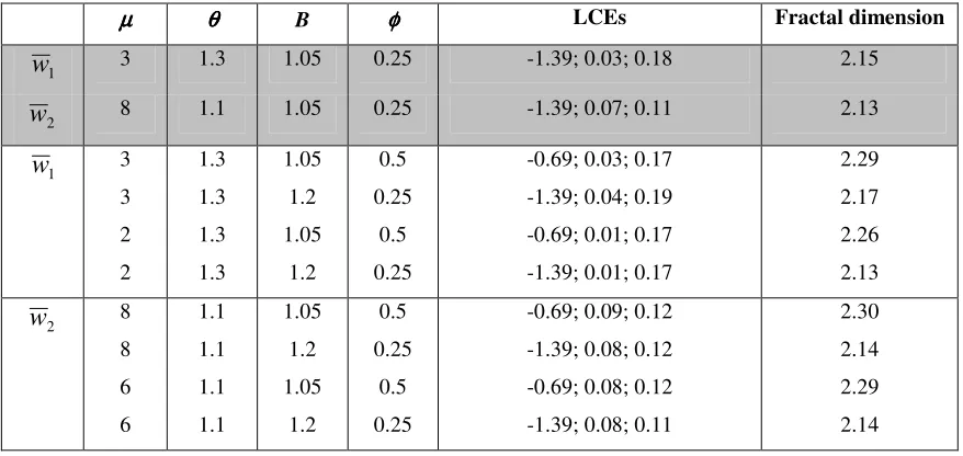
Similar attractors to the ones in figures 5 and 8 can be found in this case. Table 3
discusses the degree of chaoticity that various combinations of parameters allow for.
µµµµ θθθθ B φφφφ LCEs Fractal dimension
1
w 3 1.3 1.05 0.25 -1.39; 0.03; 0.18 2.15
2
w 8 1.1 1.05 0.25 -1.39; 0.07; 0.11 2.13
1
w 3
3 2 2
1.3 1.3 1.3 1.3
1.05 1.2 1.05
1.2
0.5 0.25
0.5 0.25
-0.69; 0.03; 0.17 -1.39; 0.04; 0.19 -0.69; 0.01; 0.17 -1.39; 0.01; 0.17
2.29 2.17 2.26 2.13
2
w 8
8 6 6
1.1 1.1 1.1 1.1
1.05 1.2 1.05
1.2
0.5 0.25
0.5 0.25
-0.69; 0.09; 0.12 -1.39; 0.08; 0.12 -0.69; 0.08; 0.12 -1.39; 0.08; 0.11
[image:19.595.79.518.424.632.2]2.30 2.14 2.29 2.14
Table 3 – LCEs and fractal dimensions for the system with endogenous technology.
Note that now we are dealing with a three dimensional system, and therefore three
LCEs are jointly computed. Note, as well, that the third equation that we have
introduced relates to a process of knowledge accumulation under decreasing returns,
and thus stability prevails in what concerns the new dimension we add. As a result, one
found in the exogenous technology case. In table 3, various combinations of parameters
to which chaotic motion exists are considered, and we find, for all of them, that despite
taking an additional dimension into the system, the dimension of the attractor continues
to be given by a value slightly above 2. In this case, the Lyapunov dimension or fractal
dimension is given by the formula
3 2 1
2 λ
λ λ + + =
D , where the LCEs in the numerator
are the positive ones and the exponent in the denominator is the negative LCE.
Since the dynamics of technology are independent of wealth and decreasing
marginal returns prevail in the accumulation of knowledge, the technology variable
converges to a long term fixed point, independently of parameter values. Wealth
dynamics will vary with the values of the credit multiplier and other parameters, as
before, but the introduction of the technological sector reveals new possibilities for
endogenous fluctuations.
6. Conclusions
We have examined a model of financial development where constraints on credit
and a risk premium over the less wealth endowed are considered. As a result, we have
concluded that a high level of financial development has a favourable effect over the
potential to grow; nevertheless, the results also point to a perverse impact of a too loose
policy concerning credit availability, because this can lead to instability. In the proposed
framework, instability can be interpreted as a state where excess of credit conducts to a
failure of the financial system to maintain the mutual confidence in the credit market
that allows for loans with low collateral requirements.
For some levels of the credit constraint parameter, endogenous business cycles
were found, an observation that confirms the results on other studies in the field
(namely, the CJM model). We identify a link between the functioning of the credit
market and the volatility of some fundamental economic aggregates, with this link
arising from the nonlinear nature of the relation between variables, namely from the
piecewise relation between a constant marginal returns value and a varying interest rate.
Introducing an endogenous technology generation process, we have confirmed the
richness of possible long term results on a model that never loses its endogenous growth
character; the economy’s long run growth rate is always constant on average (because
circumstances of the financial markets push the setup to a long term result where the
time path of the growth rate fluctuates around a constant mean.
References
Aghion, P.; G. M. Angeletos; A. Banerjee and K. Manova (2005). “Volatility and
Growth: Credit Constraints and Productivity-Enhancing Investment.” NBER
working paper nº 11349.
Aghion, P.; P. Bacchetta and A. Banerjee (2000). “A Simple Model of Monetary Policy
and Currency Crises.” European Economic Review, vol. 44, pp. 728-738.
Aghion, P.; P. Bacchetta and A. Banerjee (2001). “Currency Crises and Monetary
Policy in an Economy with Credit Constraints.” European Economic Review, vol.
45, pp. 1121-1150.
Aghion, P.; P. Bacchetta and A. Banerjee (2004). “Financial Development and the
Instability of Open Economies.” Journal of Monetary Economics, vol. 51, pp.
1077-1106.
Aghion, P.; A. Banerjee and T. Piketty (1999). “Dualism and Macroeconomic
Volatility.” Quarterly Journal of Economics, vol. 114, pp. 1357-1397.
Aghion, P.; P. Howitt and D. Mayer-Foulkes (2005). “The Effect of Financial
Development on Convergence: Theory and Evidence.” Quarterly Journal of
Economics, vol. 120, pp. 173-222.
Amable, B.; J. B. Chatelain and K. Ralf (2004). “Credit Rationing, Profit Accumulation
and Economic Growth.” Economics Letters, vol. 85, pp. 301-307.
Benhabib, J. and R. H. Day (1981). “Rational Choice and Erratic Behaviour.” Review of
Economic Studies, vol. 48, pp. 459-471.
Bernanke, B. and M. Gertler (1989). “Agency Costs, Net Worth, and Business
Fluctuations.” American Economic Review, vol. 79, pp. 14-31.
Blackburn, K. and V. Hung (1998). “A Theory of Growth, Financial Development and
Trade.” Economica, vol. 65, pp. 107-124.
Boldrin, M.; K. Nishimura; T. Shigoka and M. Yano (2001). “Chaotic Equilibrium
Dynamics in Endogenous Growth Models.” Journal of Economic Theory, vol. 96,
pp. 97-132.
Caballé, J.; X. Jarque and E. Michetti (2006). “Chaotic Dynamics in Credit Constrained
Emerging Economies.” Journal of Economic Dynamics and Control, vol. 30, pp.
Christiano, L. and S. Harrison (1999). “Chaos, Sunspots and Automatic Stabilizers.”
Journal of Monetary Economics, vol. 44, pp. 3-31.
Christopoulos, D. K. and E. G. Tsionas (2004). “Financial Development and Economic
Growth: Evidence from Panel Unit Root and Cointegration Tests.” Journal of
Development Economics, vol. 73, pp. 55-74.
Day, R. H. (1982). “Irregular Growth Cycles.” American Economic Review, vol. 72,
pp.406-414.
Demirguç-Kunt, A. and R. Levine (2001). Financial Structure and Economic Growth.
Cambridge, MA: MIT Press.
Gomes, O. (2006). “Routes to Chaos in Macroeconomic Theory.” Journal of Economic
Studies, vol. 33, pp. 437-468.
Grandmont, J. M. (1985). “On Endogenous Competitive Business Cycles.”
Econometrica, vol. 53, pp. 995-1045.
Guo, J. T. and K. J. Lansing (2002). “Fiscal Policy, Increasing Returns and Endogenous
Fluctuations.” Macroeconomic Dynamics, vol. 6, pp. 633-664.
Harrison, P.; O. Sussman and J. Zeira (1999). “Finance and Growth: Theory and New
Evidence.” Board of Governors of the Federal Reserve System, Finance and
Economics Discussion Series, nº 99-35.
Kaplan, J. L. and J. A. Yorke (1979). “Chaotic Behavior of Multidimensional
Difference Equations.”, in H.-O. Peitgen and H.-O. Walter (eds.), Functional
Differential Equations and Approximations of Fixed Points, Springer: Berlin, p.
204.
Khan, A. (2001). “Financial Development and Economic Growth.” Macroeconomic
Dynamics, vol. 5, pp. 413-433.
King, R. and R. Levine (1993). “Finance and Growth: Schumpeter Might Be Right.”
Quarterly Journal of Economics, vol. 108, pp. 717-737.
Kyotaki, N. and J. Moore (1997). “Credit Cycles.” Journal of Political Economy, vol.
105, pp. 211-248.
Levine, R. (1997). “Financial Development and Economic Growth: Views and
Agenda.” Journal of Economic Literature, vol. 35, pp. 688-726.
Levine, R. (2005). “Finance and Growth: Theory and Evidence.” in P. Aghion and S. N.
Durlauf (eds.), Handbook of Economic Growth, Amsterdam: Elsevier, pp.
865-934.
Medio, A. and M. Lines (2001). Nonlinear Dynamics: a Primer. Cambridge, UK:
Morales, M. F. (2003). “Financial Intermediation in a Model of Growth Through
Creative Destruction.” Macroeconomic Dynamics, vol. 7, pp. 363-393.
Nishimura, K.; G. Sorger and M. Yano (1994). “Ergodic Chaos in Optimal Growth
Models with Low Discount Rates.” Economic Theory, vol. 4, pp. 705-717.
Schmitt-Grohé, S. (2000). “Endogenous Business Cycles and the Dynamics of Output,
Figures
Figure 1 – Local dynamics around w1.
Figure 2 – Local dynamics around w2.
-2
Tr(J) 1
Det(J)=1
Det(J)
1+Tr(J)+Det(J)=0 1-Tr(J)+Det(J)=0
Tr(J) 1
Det(J)=1
Det(J)
[image:24.595.120.480.148.345.2]Figure 3 – Bifurcation diagram (w~t;µµµµ), for w =w1.
Figure 4 – Time series of w~t (µµµµ=1.5), for w =w1.
[image:25.595.165.425.539.722.2]Figure 6 – Bifurcation diagram (w~t;µµµµ), for w =w2.
Figure 7 – Time series of w~t (µµµµ=3), for w =w2.
[image:26.595.167.426.539.720.2]Figure 9 – Bifurcation diagram (w~t;µµµµ), for w = w1 and with endogenous technology.
[image:27.595.178.426.299.480.2]