Derivatives pricing in a Markov chain jump diffusion setting

(1)

D eriva tives P ricin g In a

M a rk o v Chain Jum p-D iffusion

S e ttin g

i

1

S h a o u l N a th a n

A thesis submitted in fulfilment of the requirements for the degree of

D o c t o r o f P h il o s o p h y

To The

D e p a r t m e n t o f S t a t i s t i c s

L o n d o n S c h o o l o f E c o n o m ic s

U n i v e r s ity o f L o n d o n

(2)

UMI Number: U 1 9 4997

INFORMATION TO ALL U SE R S

The quality of this reproduction is d ep en d en t upon the quality of the copy subm itted.

In the unlikely even t that the author did not sen d a com plete m anuscript

and there are m issing p a g e s, th e se will be noted. Also, if material had to be rem oved, a note will indicate the deletion.

Disscrrlation Publishing

UMI U 194997

Published by ProQ uest LLC 2014. Copyright in the Dissertation held by the Author. Microform Edition © ProQ uest LLC.

All rights reserved. This work is protected against unauthorized copying under Title 17, United S ta tes C ode.

ProQ uest LLC

789 East E isenhow er Parkway P.O. Box 1346

(3)

(4)

m

( . r w a r y

dtiubi, juiwy Ljt Pohücal and Économe Science

T o a

Dedicated to m y loving

(5)

Acknow ledgem ents

I would like to offer my deep gratitude to Dr. Angelos Dassios for his expert

supervision and guidance over the course of my Ph.D, as well as for his in

spiration during my undergraduate studies, which motivated me to continue

and perform this research. Many thanks to all the Department of Statistics

(6)

(7)

A bstract

In this work we develop a Markov Chain Jump-Diffusion (MCJD) model,

where we have a financial market in which there are several possible states.

Asset prices in the market follow a generalised geometric Brownian motion,

with drift and volatility depending on the state of the market. So for example,

one state may represent a bull market where drifts are high, whilst another

state may represent a bear market where where drifts are low. The state

the market is in is governed by a continuous time Markov chain. We add to

this diffusion process jumps in the asset price which occur when the market

changes state, and the jump sizes are dependent on the states the market is

transiting to and transiting from. We also allow the market to transit to the

same state, which corresponds to a jump in the asset price with no change

to the drift or volatility.

We will develop conditions of no arbitrage in such a market, and methods

for pricing derivatives of assets whose prices follow MCJD processes. We will

also consider Term-Structure models where the short rate (or forward rate)

(8)

Table o f C ontents

Table o f C ontents i

N o ta tio n iv

1 Introduction 1

1.1 General In tro d u c tio n ... 1

1 . 2 Order of W o rk ... 4

1.3 P re lim in a rie s ... 5

1.3.1 The Markov Chain M a rk e t... 5

1.3.2 Properties of the Model ... 8

2 T he E quity M odel 14 2.1 In tro d u ctio n ... 14

2.2 The M o d el... 14

2.3 Risk-Neutral M easure...21

2.3.1 Change of M e a s u re ...22

2.3.2 Martingale M easure...28

2.4 Replicating Portfolios...32

2.5 Derivatives P r i c i n g ...37

2.5.1 Interest-Rate D erivatives... 44

3 N um erical M ethod s for th e Equity M odel 48 3.1 In tro d u ctio n ... 48

(9)

11

3.3 Parametric methods ...65

3.3.1 Translated G a m m a ... 65

3.3.2 Polynomial Spline PDF F i t t i n g ...6 8 3.3.3 Application to the MCJD m od el... 82

3.4 Tree-Based M e th o d s ...84

3.4.1 Trinomial T r e e s ...84

3.4.2 Multinomial Trees ... 95

3.5 Monte Carlo S im u la tio n ...101

3.6 Comparison of Perform ances... 104

4 In terest-R ate T heory 106 4.1 In tro d u ctio n ... 106

4.2 The M o d el...108

4.3 Short-Rate M o d e ls ... 116

4.3.1 Derivatives p r i c i n g ... 117

4.3.2 Models of the Short R a te ... 123

4.3.3 Market Com pleteness... 132

4.4 HJM M odels... 135

4.4.1 Martingale M easure... 137

4.4.2 Forward Rate M e a s u re ... 142

4.4.3 Derivatives P r ic i n g ... 146

4.4.4 Market Com pleteness... 158

4.4.5 Replicating Portfolios... 161

4.5 Credit Derivatives... 164

4.5.1 Corporate B o n d s ...164

4.5.2 Credit Default S w a p s... 169

5 N um erical M ethod s for In terest-R ate M odels 174 5.1 In tro d u ctio n ... 174

5.2 Trinomial Trees for Short-Rate M o d e ls ... 177

5.3 Multinomial Trees for Short-Rate M o d els... 184

5.4 Monte Carlo Simulation for Short-Rate M odels... 191

5.5 Monte Carlo Simulation for HJM M o d e ls... 195

5.6 Binomial Trees for HJM M o d e ls... 197

(10)

Ill

B A D istributional R esu lt for S hort-R ate M odels 208

(11)

N otation

During the course of this work there will be the need to define many terms

and symbols in order to develop all the theory. In order to assist the reader

we have listed below some of the most commonly used terms, as well as the

page number where they are first defined and a brief description of what they

are used to represent. We have also included a list of matrices.

Term Page no. Description

Yt 5 Markov chain representing the state of the market at time t.

S 5 The set of possible states the market can be in which

can take values 1, . . . , n .

n 5 Total number of states in the market .

j 5 Subscript denoting the state of the market, j Ç: S.

k 5 Subscript denoting the state of the market, k E S.

5 The transition intensity from state j to state k.

(12)

6 The total number of times the market has transited from

state j to state k up until time t.

Nt 6 The total number of transitions of the state up to time t.

1} 7 Indicator variable taking the value 1 if the market is

in state j at time t and 0 otherwise ,

8 The probability at time 0 th a t the market is in state k at time t, given that at time 0 it is state j .

8 The total expected time spent in state k in the interval

[0, t], given th at at time 0 the market is in state j.

J 9 An T + 1 dimensional row vector representing the jump

sequence of the first x jumps.

Dt 9 Markov chain used for phase-type distributions.

w 1 1 Subscript denoting the state of the Markov chain

Dt-w = 1 ,... ,x 1 .

pii-jx+içp^ 12 The probability of observing jump sequence J ' in time T.

13 The probability of transiting from state j to state k conditional on a transition occurring.

r 15 Total number of Brownian motions.

b 15 Subscript denoting number of Brownian motion. 6 = 1 , . . . , r.

W} 15 Value of Brownian motion number b at time t .

17 The jump size of asset i when transiting from state j to

state k. The i may be suppressed when there is only one asset.

(13)

VI

Tj 19 The rate of interest whilst in state j .

Si^t 20 The price of asset i at time t. The i may be suppressed

when there is only one asset .

Si^t 20 The discounted price of asset i.

fiij 20 The drift of asset i whilst in state j . The i may be

suppressed when there is only one asset.

ai^bj 20 The volatility of asset i due to Brownian motion b

whilst in state j . The i may be suppressed when there is only one asset. The b may be suppressed when there is only one Brownian motion.

fiij 22 Drift of asset i in state j under transformed

(risk-neutral) measure.

$bj 22 Addition to the drift for Brownian motion 6 in state j .

25 Transformation to transition intensity from state j to

state k under transformed (risk-neutral) measure.

rt 108 The value of the short rate at time t.

108 The drift of the short-rate process at time t.

a {t,Y t-) 108 The volatility of the short-rate process at time t.

7’’(t, Y t-,Y t) 108 The size of the jump in the short-rate process at

time t.

p(t, T) 108 The value of a zero-coupon bond at time t expiring at

time T.

m{t, T, Yt-) 108 The drift of the zero-coupon price process.

v{t,T , Yt-) 108 The volatility of the zero-coupon price process.

7^(t, T, Y t-,Y t) 108 The size of the jump in the value of the zero-coupon

(14)

vil

108 The forward rate between times t and T.

a {t,T ,Y t-) 108 The drift of the forward-rate process.

b { t,T ,y t-) 108 The volatility of the forward-rate process.

't/it,T ,Y t.,Y t) 108 The size of the jum p in the forward-rate process.

A { t,T ,Y t-) 113 Minus the integral of a {t,T ,Y t-).

B { t,T ,Y t-) 113 Minus the integral of b(t,T, Yt-).

r f{ t,T ,Y ,.,Y t) 113 Minus the integral of Yt-).

P{0,T) 124 Empirical bond prices.

f{ 0 ,T ) 124 Empirical forward rates.

(15)

Vlll

Matrix Page no. Description

D (a) 2 1 m x m m atrix with elements of a down the principal

diagonal where a G

gmxl

2 1 Vector of discounted stock prices.

UJixl _{2 1} _{Vector of drifts.}

^mxr _{2 1} _{Matrix of volatilities.}

w r ' 2 1 Matrix of Brownian motions.

T'TTixn

'■j 2 1 Matrix of jump sizes.

N i 2 1 Vector of counting processes.

ÛJixl _{2 2} _{Vector of drifts under transformed (risk-neutral) measure.}

w r ' 2 2 Vector of Brownian motions under the changed

(risk-neutral) measure.

Anxl ₂₇ _{Vector of transition intensities.}

^nxl ₂₇ _{Vector of transformations to transition intensities under}

(16)

C hapter 1

Introduction

1.1

G en era l In tr o d u c tio n

Over 30 years ago Black and Scholes produced their seminal paper Black

and Scholes [1973], which together with Merton [1973] paved the way for the

development of mathematical finance as we know it. Their papers were based

on the assumption th at the price of the underlying asset follows the behaviour

of a diffusion process, most notably a geometric Brownian motion. Another

watershed was the development of the Arbitrage Pricing Technique in Ross

[1976] and Ross [1978], and the martingale approach to arbitrage pricing

developed in Harrison and Kreps [1979] and Harrison and Pliska [1981].

The Black-Scholes model has become very popular due to its simplic

ity in th at it quantifies risk through a single constant volatility parameter.

(17)

1.1 General Introduction 2

totally adequate when attem pting model the behaviour of today’s complex

financial markets, and this accusation has been supported by various empir

ical studies (for example see Bakshi et al. [1997]). There have subsequently

been many attem pts to modify this model and relax its over-simplistic as

sumptions. Stochastic volatility models have been extensively studied where

the volatility is allowed to evolve over time (see Hull and White [1987], Stein

and Stein [1991] and Heston [1993], or alternatively for a synopsis see Fouque

et al. [2 0 0 0]).

On an alternate front, there have been attem pts to develop models which

incorporate jumps into the asset price behaviour. Such jumping behaviour

in asset prices has been supported by empirical evidence such as in Ball and

Torous [1985] and Jorion [1988]. Pure jump processes were developed in pa

pers such as Merton [1976] and Bjork et al. [1997]. A natural extension to

these models are processes th at include both a diflFusion part and a jump

part, known as jump-diffusion processes, such as in Andersen and Andersen

[2000] and Madan [2001]. Many other varying models have been developed

to try to improve on the Black-Scholes model, although in their increased

sophistication they sacrifice a lot in terms of ease of calculation, as well as

intuitiveness of the models. This last factor is fairly important, as any model

which requires a so-called ‘rocket scientist’ to understand is unlikely to be

used widely by practitioners. They prefer to employ more simplistic models

(18)

1.1 General Introduction 3

In this work we shall develop a different type of Jump-diffusion model which

we shall call a Markov Chain Jump-Diffusion Model (MCJD). The motiva

tion for this lies behind two papers where totally different models have been

developed. Firstly, in Norberg [2003] a pure-jump process is considered where

the market is driven by a continuous-time homogenous financial market. Al

ternatively, in Runggaldier [2003] a jump-diffusion process is developed where

the jumps are modelled by a marked point process.

In our MCJD model we consider a market in which there are several states

of the market. Asset prices in the market follow a generalised geometric

Brownian motion, with drift and volatility depending on the state of the

market. So for example, one state may represent a hull market where drifts

are high, whilst another state may represent a bear market where drifts are

low. The state the market is in is governed by a continuous-time Markov

chain. We add to this diffusion process jumps in the asset price which occur

when the market changes state, and the jump sizes are dependent on the

states the market is transiting to and transiting from. We also allow the

market to transit to the same state, which corresponds to a jump in the

asset price with no change to the drift or volatility.

This model constitutes a stochastic drift and volatility model as these

parameters are allowed to change, as well as being a jum p process. It is

very intuitive to see how this model may represent the behaviour of financial

assets, as it is widely recognized th at there are trends in the market, and

(19)

1.2 Order o f Work 4

the advantages of stochastic volatility models and jumps processes in th at

it should describe more accurately the behaviour of financial assets, and at

the same time regulates these features in a restricted sense so as to facilitate

pricing, and hopefully making intuitive sense.

1.2

O rder o f W ork

In the conclusion of this chapter we will describe the market characteristics

common to all the subsequent models, and develop several results concerning

Markov chains which will prove useful in our subsequent investigations.

In chapter 2 we develop the Equity model where asset prices follow our MCJD

model. We will deal with issues of completeness, replicating contingent claims

and finally pricing derivatives.

In chapter 3 we shall develop and compare various numerical methods for

pricing derivatives on the assets described in chapter 2. We will look at a

particular example and see how all the methodologies had priced call options

on this asset.

Chapter 4 sees us turning our attention to Term-Structure models where

we will use our MCJD model to describe the behaviour of the short rate for

(20)

1.3 Preliminaries 5

issues regarding completeness and derivative pricing for these models, as well

as parameter estimation.

Finally in Chapter 5 we will develop numerical methods for pricing the

interest-rate derivatives developed in chapter 4.

To try to make reading this thesis as easy as possible for the reader, we

have also included a notation page which includes many of the terms and

symbols th at are used repeatedly throughout this work.

1.3

P re lim in a r ies

1.3.1

T h e M arkov C hain M arket

As mentioned above, in this work we shall be considering a market in which

there are n states represented by the continuous-time Markov chain (lt)t>o

with finite state space «S = {1. . . n}. The process Yt transits between states j

and k where j , k E S with intensity A-^*, so th a t the generator of this process

is given by

G =

-Â1 . . A'" \

■ -Â " /

(21)

where This process is time-homogeneous, so th a t for j ^ k

we have th at

Pr[y(+rf( = k \ Y t = i \ = + o{dt). (1.3.2)

We also have that

> 0,

and we are assuming there can be at most one transition for any small length

of time dt.

Let us add to the above Markov chain the ability to tr a n s it to the same

state, the probability of which is given by X^^dt. This should not be confused

with the probability of re m a in in g in the same state which has probability

equal to 1 — + o{dt). The motivation for doing this will become

clear in section 2.2, We can therefore regard this extended process as being

a multivariate point process, with state-dependent intensity vector Aj given

by

= V j € S .

Define Nl as being the number of transitions from state j to state k up to

time t, so th at for j ^ k

= |{^; 0 < 8 < t , Yg = k , Yg- = j} \,

whilst is the number of times the process was in state j and tr a n s ite d

to the same state. Nt denotes the total number of transitions up to time t:

(22)

where we set Nq = 0. We shall call this point process the jump process and

its intensities the jump intensities, as opposed to the transition process given

in 1.3.1.

We make the assumption of non-explosion, so th a t iVt < oo for t > 0

(similarly < oo V j,k ) , and assume Nt is defined on some probability

space (n, P ) with filtration to which Nt is adapted. This process can

be characterised as a doubly stochastic Poisson process with state-dependent

intensity At, where

A. = A(y,) = ^ l A , / / , (1.3.3)

jes

1 is a 1x4 row vector with all entries equal to 1, and l} is the indicator

variable which takes values

{ 0 otherwise.

The expected time spent in state j before transiting out is therefore expo

nentially distributed with parameter (lAj — A-^-^). We shall denote the times

at which each of these Nt jumps occur by t i , . . . ,tN^. Finally, we shall set the

process Yt to be left continuous and hence it will also be prévisible. In the

remainder of this work we shall denote prévisible state-dependent processes

(23)

1.3.2

P ro p erties o f th e M od el

We will now derive some properties of this model which we will make use

of in the forthcoming chapters. In order to do this, let us first write the

following definition (for example see Grimmett and Stirzaker [2 0 0 1]):

D efin itio n 1.3.1. Given a Markov chain setting described in section 1.3,1,

the probability of being in state k at time t given th at at time 0 we were in

state j for j , k e S is given by

= P[yt = k \Y o = j].

The probability pj*' is then given by

pI^ = P 'exp {tG^} I*’

°° ty

where 1^ is the n-dimensional column vector with the entry equal to 1

and all other entries equal to 0, and G is the generator defined in (1.3.1). We

denote the transpose by '. Let us also define the expected total time spent

over the interval [0, t] in state k, given at time 0 we are in state j , by

J 3 = 0

(24)

1.3 Preliminaries

We therefore have

In order to perform many of the calculations in subsequent chapters, we

will need to condition on the path taken by the Markov chain Yt. We will

now derive some results when conditioning on this path, which we will make

use of when pricing derivatives later on.

Let us condition on the Markov chain Yt following a given path. Suppose

the Markov chain starts in state j i , and th at the first x + l transitions of the

Markov chain (where a jump to the same state is considered a transition) are

at times t i , . . . , tx+i- Let the jump sequence (and hence state of the Markov

chain) of the first x of these jumps be represented by the x + 1-dimensional

row vector J" = { j i ,.. . ,jx+i}- Under this setup, we shall now calculate the

probability the Markov chain is in each state at any time t G [0, T]. In order

to do this we shall set up our model as a phase-type distribution (see As-

mussen [2000] or O ’Cinneade [1990]).

Constructing a phase-type distribution involves representing this condi

tional Markov chain as a different Markov chain Dt which has generator Qj-,

where the subscript shows dependence on the path we are conditioning on.

We shall use the subscripts j and k to denote states of the original Markov

(25)

Whilst Yt is in state ji, it transits to state j2 with intensity . Similarly,

whilst in state j'2 it transits to state js with intensity and so on, until

Yt arrives at state jx+i- Since we are not conditioning on any subsequent

transitions, the transition intensity out of state jx+i is the total intensity for

transiting out of state jx+i given by where A^=+^^ This

conditional Yt process can be represented by the continuous-time Markov

chain Dt where Dt G { l , . . . , x - | - 2 } , which has generator Q j given by the

X -f- 2-dimensional square matrix below:

Q j =

.\h32 \h h 0 0

0 A^'2J3 0

0 0 -A^=^4

0

. \ 3 x j x + \ ^ i x j ’x + 1 Q

0 0 0

If all transition intensities are different then Qj- can be diagonalised,

which would simplify many of the calculations below. Let us now write the

following lemmas:

L em m a 1.3.2. We will now calculate the value of conditional on the

jump sequence J . Suppose we have Dq = 1. Using (1.3.5) the probability

that Dt = a; 4-1 , i.e. that we have had exactly x transitions up until time T

(26)

is given by

°° 'T'y

= z + = (1.3.7)

y=0

where once again V is the x + 1-dimensional column vector with all entries

equal to 0 and thej^^ entry equal to 1. Conditioning on Dt = x-\-l being true,

we can further see that the probability of being in state w for w = 1 ,... ,x-{-l

at time t where t G [0, T] is given by

_

(E ” o

(1.3.8)

P[Dt — w\Dt — X 1] — v^oo Ty-iifrïV

We can re-write (1.3.8) as

P[D, = w\Dt = x + 1] = . L i ^ --- (1-3.9)

where

tvi (T -y i W

We now have that the conditional probability at time t of being in state k

of our Markov chain Yt, given that we start in state j at time 0 is given by

p i^ \J = ^ 2 ~ = x -\-1]. (1.3.10)

{ w : j w = k }

(27)

K M - 2^ v “ ï ï i i ' o i ' i * + i ■

{ w : j w = k } 2 - /J /—0 y l

We now also define to be the expected total time spent in state k so

that

Pt \ J = f (1.3.12)

Jt=o

We can integrate (1.3.11) to get

{ w : j w = k } 2 - ^ y — O y \ J

where

j ’Cyi+w+i) Z =

f o i + 2 / 2 + 1 ) ! ’

□

L em m a 1.3.3. We will now calculate the probability of observing jump se

quence J = ( j i , . . . , jx+i) an interval [0,T], which we will denote by

(28)

Q j =

-Âj 0 0

0 -Â^ 0

0 0 - X i AJ3J4

0 0

0 0 0 0

-A^ ^jxjx+i

0 —X^^+^ A^'+^

0 0 0

where as previously we have X^ = Y!!k=i weZZ as X^^ = X^ — A^*. We

therefore have

j y

U y '

(1.3.14)

□

Finally, we have the following definition:

D efin itio n 1.3.4. When in state j and given th a t a transition will occur,

the probability th at the process will transit to state k is given by

= P[lt+df = k\Yt = j. Transition has occurred]

(1.3.15)

\jk AJi 4-. . . 4- A;"

for &== 1, . . . ,n, so th at we also have th at Ylk=iP^^ ~ 1

-The usefulness of these lemmas will soon become apparent. We shall now

(29)

Chapter 2

The Equity M odel

2.1

In tr o d u ctio n

In this section we will begin by introducing the model, and then use the Black-

Scholes methodology to price derivatives whose underlying is represented by

this model. We will obtain a risk-neutral measure under which our model

will be a martingale, find a self-financing replicating strategy, and then finally

develop an equation to price the derivatives.

2.2

T h e M o d el

Our market contains assets whose price processes are dependent on the state

of the Markov chain market described in the previous chapter. Suppose we

have an asset whose price process, denoted by St (where S t > 0 Vt), follows

(30)

2.2 The Model 15

a generalised geometric Brownian motion so th at

r

dSt

=

ti{Yt.)Sidt +

^

ci,(Yt-)StdW^,

(2.2.1)

6 = 1

where the W} for 6 = l . . . r are independent Brownian motions under the

probability measure P , and the drift function /x(-) and volatility functions

CTb(') are deterministic functions of the state variable Yt-. Note th at the

mean and drift functions are dependent on t — as they are predictable. The

price process of an asset behaving according to this model will therefore have

constant drift and volatilities until a transition occurs in our Markov chain.

We so far have the Markov chain and the diffusion part of our model,

and we will now add the jump part. We shall add to equation (2.2.1) a jump

process as follows. Suppose the Markov chain Yt has transited from state j to

state k. Let 7^*^ be a random variable representing the size of the jump in the

asset price due to this transition, such th at 7/*^ > — 1 Vt. Being dependent

on t and not t — means th at 7^ will not be predictable. Adding this random

variable to (2.2.1) we get

dSt = St

6= 1 j = l fc = l

(2.2.2)

where the counting process is defined as in section 1.3.1. This implies

(31)

2.2 The Model 16

transition of the Markov chain has occurred (which includes a transition to

the same state). We shall assume th at the jumps and the Brownian motions

are independent. Note th at forcing 7/*^ to be greater than or equal to —1

ensures that the asset price will never jump to a negative value. We also

have th at

Pr[St2 — = 0] = 1 Vt2 > ti;

so th at once the asset has lost all of its value it can never regain it.

We are now left with the task of assigning a distribution to 7/*^. We will

confine ourselves to using a distribution with a finite event space, because

should the event space be infinite we would then need an infinite number of

assets to obtain a risk-neutral measure, as shall be seen later on.

Consider a model under which for each transition from state j to k there

are I possible jump sizes given by where all the jump sizes

are finite and greater than -1. So given th at a jum p from state j to state k

occurs, the jump size is represented by 7/^ which has distribution

with probability pj*

i t =

P t with probability

for all j , k £ S and where = 1 Vj, k. W ith this setup we can

replicate practically any distribution for 7/^ with a suitable choice of I.

We are also able to represent this model in a different way. Our model

(32)

2.2 The Model 17

I possible jump sizes in the asset price. We could however represent each of

these jump sizes as their own state in the market, all of which have the same

drift and volatility but only with differing jump sizes. We would then be left

with a model where there are n x I states, with only one possible jump size

between any two given states. For the rest of this work, we will therefore

consider models where there is only one possible jump size when transiting

from state j to state k so th at 7^^ = 7-^^. All the results which will be devel

oped will therefore also hold true for models where there are more possible

jump sizes between any two states, since this would simply correspond to a

model with more states in the market.

Now th at we have all the components of our model we can write the fol

lowing proposition:

P ro p o sitio n 2.2.1. Assume that between times [0, t] jumps occur at times

£1, . . . ,tjVf The solution to (2.2.2) is given by the following exponential for

mula:

St = Soexp ^ « t K F , - )

j

ds + ^ M Y s-)d W ^

+ /* è è I . (2-2.3)

•/»=<> j=i k=i J

Proof. The result can be obtained by applying the standard Itô formula

(33)

2.2 The Model 18

Calculus (see Appendix A4 in Brémaud [1981]). Alternatively, it can be ob

tained from the generalised Itô formula as in Runggaldier [2003] or Apple-

baum [2004].

□

This model has a lot of appeal because it is describes the manner in

which many of the world’s financial markets behave: a stable period of fluc

tuation and drift, followed by a sudden change in the market conditions.

This shock to the system causes asset prices to jump and there to be new

levels of drift and volatility. It is particularly apt to fit such a model to less

liquid markets, where price behavior is generally stable until external stimuli

cause temporary shocks to the system, whereby a new equilibrium is reached.

We shall now introduce into our market a numéraire in the form of a bank

account process Bt, which grows by a predictable state-dependent interest

rate r{Yt-). We will assume r{Yt-) > 0 Vt. This bank-account process has

dynamics

dBt = r{Yt-)Btdt,

which has solution

Bt = exp r ( y ;_ ) d s |

(34)

2.2 The Model 19

We can now define the discounted asset price process St as

St = S t / B t ,

which has dynamics

dSt = St H Y t- ) - r ( y , . ) ] dt + J2 + Ë Ë

6= 1 j=l fc=l

(2.2.4)

Since the drift, volatility and interest-rate functions are only dependent

of the value of Yt-, we can therefore denote them whilst in state j as being

/ij, (Tb,j and rj respectively for all j E S . We can therefore write equation

(2.2.4) more simply as

dSt = S t ^ i i ;=i

(% - r i ) d t + J 2 + É

6= 1 fc=l

(2.2.5)

where 1} is the indicator variable th at the market is in state j at time t, and

is the number of times th at the Markov chain has transited from state

j to state k as described in section 1.3.1.

We can now write the following corollary:

(35)

2.2 The Model 20

is the solution of (2.2.5), can he obtained using the same manner as for the

undiscounted price process in proposition 2.2.1 to give

St = S^exp}^ / ^ = 0 j=\

{fJ'j ~ '^3 - ^bjdW t

A

6=1

/

6=1

k = l

(2.2.6)

□

Finally, our market consists of a set of m assets M. = ,m }, whose

discounted price processes are all described by equations similar to (2.2.5),

although with different drift, volatility and jump sizes. For asset z G A^, let

the price process be denoted by Si^t and the drift and volatihty functions by

Uij and (Ti^bj respectively, as well as the jump sizes by for and all j, k G S .

We can now re-write the discounted asset-price dynamics equation (2.2.5) for

all assets z G Ad as

3 = 1

ilJ'ij - '>^j)dt + (JifijdWt + dN(^

6= 1 fc=l

(2,2.7)

or alternatively in m atrix form

dS, = //D (S ,) [(Uj - V"Tj)dt + S jd W , + Tj-dNl] , (2.2.8)

(36)

2.3 Risk-Neutral Measure 21

where D (a) is an m x m diagonal matrix when a E with the elements

of a down the principal diagonal and 0 elsewhere, 1”^ is an m x 1 column

vector of I ’s, and we also define the following matrices:

g m x l

I j m x l

y^ m xr

~ 6 = l.,.r

•p m x n

~ {"Ti } i = l .. ,m fe=l,„n

N J "X I

= { N t } k = l . . . n

-2.3

R isk -N e u tr a l M ea su re

We will now establish the set of price processes which do not permit any arbi

trage opportunities. In order to do this, we will first develop a Girsanov-type

change of measure. We will then proceed to finding the necessary conditions

under which this change of measure is a martingale measure, th at is a mea

sure under which the discounted asset-price processes in equation (2,2,7) are

martingales. It was shown by Dybvig and Huang [1988], as well as Harrison

and Kreps [1979] and Harrison and Pliska [1981], th a t the existence of such a

measure is equivalent to a lack of any arbitrage opportunities in a finite-state

(37)

2.3.1

C hange o f M easure

The main tool for transforming processes into martingales is Girsanov’s the

orem (or Cameron-Martin-Girsanov theorem), which is discussed in the con

text of stochastic differential equations in 0 ksendal [2 0 0 0], or for its use in

mathematical finance see Bingham and Kiesel [2004] . This is done by induc

ing a change in the drift of a Wiener process by choosing a suitably different

probability measure. We will need to adapt the standard version of this the

orem for use in our model, but let us begin by stating this classic theorem

for when St follows the process defined by equation (2.2.1), th a t is without

any jumps.

T h e o re m 2.3.1 (G irsa n o v ). Suppose we have a financial market as de

scribed in section 1.3.1 where there are no jumps. The prices of the m assets

in this market S{t) G follow an ltd process defined on the probability

space (ÇI, 1F,P) of the form

n

dS, = J 3 //D ( S ,) [ U jd t + S ,d W ,], t < T , (2.3,1) J=1

where the notation is as defined above. Suppose predictable processes mxl

and exist where

(38)

- U j - \Jj,

and where Q j satisfies Novikov’s condition

Let

E exp 1 r'^ ”

- d

< oo.

d i t = liLtQ'jdNVit), Lo = 0,

j = i

(2.3.2)

(2.3.3)

where

and

dQt = LtdPt

on T . We can now define

n t n

' - i s

W t . = y I^.Qjds-\-Wt] t < T ,

(2.3.4)

where W t is a b-dimensional Brownian motion w.r.t. the equivalent proba

bility measure Q. We can now represent the process Sf in terms of this new

Brownian motion under Q as follows:

n

dSt = 5 3 [ d jd t + S jd W (i)] .

(39)

Note th a t if m = b and 2^^"^ is invertible, then the process Q j defined

in equation (2.3.2) is uniquely given by

e , = s - i u , - Û , ].

We can now set the process St to be a martingale by letting Û j = 0 for

all j G S. For the above model to be complete we require the existence of a

unique martingale measure, and hence a unique Q j for all j G S . For this to

be achieved in the no-jumps case above, we require th at the number of assets

to be equal to the number of Brownian motions, as well as the invertibility

condition above to be fulfilled. Having fewer assets than this means th at

there will be an infinite number of such measures, and more assets than

this could mean no risk-neutral measures. Either case will leave us with a

market which is either incomplete, or where there potentially exist arbitrage

opportunities.

It is interesting to note th at the number of states of the Markov chain

does not affect the number of assets required for the market to be complete.

This is because since there are no jumps in the asset prices, we can regard

the process as being a standard generalised geometric Brownian motion with

constant drift and volatilities whilst it is in a particular state.

We shall now try and extend the above theorem to include the jump process

as in model (2.2.7). To remind ourselves, when in state j the process can

(40)

it can easily be generalised) for each such transition we will take there to be

only one possible jump size in each of the asset prices. The probabihty of a

transition from state j to state k at any time t < T is X^^dt.

We will now develop a similar measure transformation as performed above

to include the jump process as in Runggaldier [2003] (see also Brémaud [1981]

and Bjork et al. [1997]):

T h e o re m 2.3.2. Consider a financial market described by equation (2.2.7).

Let . . . , be an J^t-P'f'^dictable process where > 0 y j , k E S so

that y t < T we have

n n

i = l fc=l

Define

where satisfies equation (2.3.3) above and is given by

dLf> = - l ) L f } { d N t - X^^dt). (2.3.5)

fc=l

Noting that we can have at most one jump in a time period of length dt, then

from equation (1.3.2), where we ignore the negligible term we have

E d N t = = k\Yt = i]

(41)

IVe therefore also have that

L \(2) = Ij = 1,

which together with equation (2.3.4) gives us

E ^lL t] = l,

where Lq — as the jump process and the Brownian motions are assumed

to be independent. Using (2.3.3) and (2.3.5) and this independence property,

we get for the Radon-Nikodym derivative Lt

dLt = • Lf>) = L f} d L f^ + L ? d L l^ \

which becomes

dLt = U ' E + L t- - l ) ( d N t

-j=\ fe = l

and which can then be solved to give

Lt = exp

s= 0 _j=i

Ê (1 - - i l l © j i r ) ds + & ,d W is )

.k=l

jk

k=l

We now have an equivalent probability measure Q given by

(42)

under which not only do the drifts in each state change from \Jj to \Jj such

that

Û ; = U j

-but the intensities of the jump process also undergo the transformation

Vj.fc.

□

Using this Girsanov-type transformation we thus have:

C o ro lla ry 2.3.3. Under Q, the discounted asset-price processes given in

equation (2.2.8) become

n

dSt = //D (S J [(U,- - 2 , 0 , - l ^ r j ) d t + 2 ,d W ( -k r,d N j] , (2.3.6) i=i

where W* is a b-dimensional Q martingale, and where we also have that

E [dNJ] =

where

A f i = (2.3.7)

(2.3.8)

and once again D (a) denotes the diagonal matrix with the vector a down the

principal diagonal.

(43)

2.3.2

M artingale M easure

We will now look at the conditions necessary for Q to be a martingale mea

sure, th at is th at under Q we have

Efi[dSt] = 0 Vt.

Taking expectations of equation (2.3.6) we can see th at this condition be

comes th a t for each state j we must have

U j - S jG j - l ^ r j -k = 0. (2.3.9)

Let us define the m x (r + n) augmented matrix B j as having entries for

X = 1 ,... ,m , y = 1 ,... ,{r -h n) where

SO t h a t

B;

m x ( r + n )

- E j : rjD ( A j) (2.3.10)

Similarly define the (r-l-n) x 1 augmented column vector V j as having entries

V j î o r x = l , . . . , { r - \ - n ) where

I _ f ^x,j I < X <

j y r < X <

(44)

so th at

—

( r + n ) X1

r x l

n x l

We can now re-write equation (2.3.9) as

B ;V , = - Uj].

In order for there to be unique values for and ^ j , and hence a unique

V j, we therefore require that for all j E S the matrix be invertible. Given

th a t B j is an m X (r -f n) matrix, this will clearly only be possible if we have

exactly r -hn assets so th at m = r -f- n, and th at

R a n k (Bj) = r-j-n . (2.3.11)

This result is rather intuitive as it is requiring th a t we have one asset for

each source of risk - the r Brownian motions and the n states th a t the model

could jump to. Should the above conditions hold, this would then give us

(2,3.12)

We are then left with a unique martingale measure Q, where by substituting

(45)

n

dSt = -fi D (S,) S jd W t + r , (dN i - . (2.3.13)

J = 1

Defining

equation (2.3.13) then becomes

" r 1

dSt = ^ / / D C S , ) S jd W , + Tj-dNJ i=i

(2.3.14)

where W* and NJ are both Q martingales for all j E S.

We shall now look at an example of this model.

E x a m p le 2.3.4. Consider a market where there are two possible states; a

bear market represented by state 1 in which drifts tend to be lower, and a

bull market represented by state 2 in which drifts tend to be higher. We shall

set the interest rates = T2 = 0.03. There are three assets in this market,

whose price processes have dynamics given by (2.3.6) where there is only one

Brownian motion. The drifts and volatilities under Q given by U j and S j

for j = 1,2, as well as the jump sizes given by Fj are shown in table 2 . 1

below. Suppose th a t we also have the jump intensities between each state

(46)

P eiram eters

A sse t 1

S ta te 1 S ta te 2

A sset 2

S ta te 1 S ta te 2

A sse t 3

S ta te 1 S ta te 2

D rift

V o latility

-0 . 2 0 0 0.060

0.070 0.090

0.065 0.070

0.052 0.100

0.128 0 . 0 2 0

0.070 0.120

J u m p Sizes A sset 2 A sset 3 A sse t 4

S ta te 1

S ta te 2

S ta te 1 S ta te 2

-0.170 0.800

-0.450 0.600

S ta te 1 S ta te 2

-0 . 0 1 0 0 . 2 0 0

-0.315 0.270

S ta te 1 S ta te 2

-0.410 0.600

-0.350 0.390

Table 2.1: Asset parameters and jump sizes under ‘real-world’ measure.

Using these parameter values and employing equation (2.3.12), we then

have a risk-neutral measure where the drifts and the jump intensities are

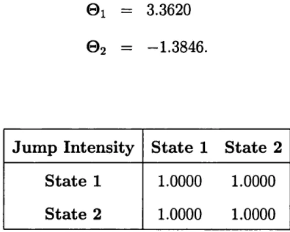
transformed to the figures shown in table 2.3, where we have

01 = 3.3620

0 2 = -1.3846.

□

J u m p In te n s ity S ta te 1 S ta te 2

S ta te 1

S ta te 2

1 . 0 0 0 0 1 . 0 0 0 0

(47)

2.4 Replicating Portfolios 32

D rift A sse t 1 A sse t 2 A sse t 3

S ta te 1

S ta te 2

-0.435

0.185

-0 . 1 1 1

0.208

-0.107

0.186

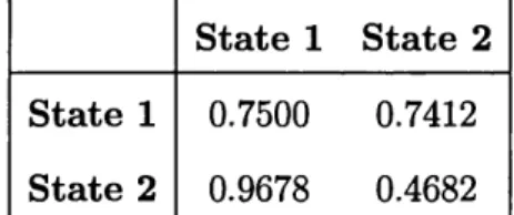
J u m p In te n s ity S ta te 1 S ta te 2

S ta te 1

S ta te 2

0.7500 0.7412

0.9678 0.4682

Table 2.3: Risk-neutral drifts and jump intensities between each state.

Once the market is complete in the sense th a t there is a unique martingale-

measure, we can invoke the completeness theorem which would imply th at

every contingent claim can be hedged by a self-financing portfofio, since there

are only a finite number of jump sizes.

We shall now proceed to show the existence of such a portfolio in our

market.

2 .4

R e p lic a tin g P o r tfo lio s

Let Xt be a contingent claim at time T, th a t is an measurable random

variable with finite expected value. Denote the price process of this claim by

Ct = BtEqlBrj}Xt |

(48)

Ct = EqIB ^^Xt I J^t] = Eq[Xt I Tt]. (2.4.1)

Suppose th at at time t the model is in state j , and we hold a portfolio

consisting of rjtj units of the cash bond and units of asset i for all i =

1, . . . , m. Let be the m x l vector of asset holdings, so th at

and T]tj must be T t — predictable. The value of the portfolio under this

strategy would then be given by

3 = 1

I tjB t + ^

i = l

The value of the discounted portfolio is

m

j=l i = l

The strategy 0 is said to be self-financing if

m

d v , * = Y , i i j=l

L t i = l

or alternatively in matrix form

3 = 1

(49)

A contingent claim Xt is said to be attainable if there exists some self-

financing replicating portfolio $ for which

Vÿ = Xt.

If any such contingent claim is being traded in the market, then in order to

avoid arbitrage we must have th at the price of this claim and its replicating

portfolio are equal, i.e.

V ? = C f (2.4.3)

By inserting equation (2.4.3) into (2.4.2), we therefore have th at in order for

the claim to be replicable by a self-financing portfolio we must have th at

n

d C t ^ Y ^ P M j d S t . (2.4.4)

i=i

Replacing (2.3.14) into (2.4.4), the strategy $ is a self-financing replicating

portfolio of the discounted claim X t if and only if

dCt = 4 $ L D ( S J [ S ; d W , + T j d N i ] . (2.4.5) J=1

Once the values of $ have been obtained, equation (2.4.5) can be used to

determine the amount held of the cash bond by

n

In section 2.5 we will calculate explicit formulas for the asset and bond hold

(50)

The market is said to be complete if every contingent claim is attainable.

Noticing th at the process (2.4.5) is also a Q-martingale, the n-factor mar

tingale representation theorem tells us th at we can represent the process Ct

as

Ct = Efi[Ct]+ f

^

Ja=0 =1

jk

. 6 = 1 fc=l

or similarly

dC, = ' £ l i j=l

jk

.6 = 1 k=l

(2.4.6)

where and are T t— predictable for all b, j and k, and where Wt and

iV/^ are Q martingales. Let the (r + n) x 1 column vector H tj have entries

TT® for a; = 1, . . . , (r + n), where

X < r

r < X < r -\- n.

To determine the values of e jj and we can compare coefficients in equation

(2.4.5) to those in (2.4.6) to give us for all j

= g;d (s, (2.4.7)

(51)

' Tj (2.4.8)

For there to be a unique replicating portfolio for the contingent claim Q ,

we therefore require the existence of a vector for every given TLtj such

th at the above equation holds. For th at to be the case, we require th at Ilf j

to be in the row space of G ' D (S J , or alternatively

R a n k = r + n. (2.4.9)

As D(Sf) is an m X m diagonal matrix it clearly has rank m. When

exploring the existence of a risk-neutral measure in section 2.3.2, we required

th at m = r -1- n, as well as the matrix B j given in equation (2.3.10) to be

invertible and hence to be of full rank. This therefore necessitates th at

R a n k ( S j) = r (2.4.10)

R a n k (rjD (A j)) = n. (2.4.11)

Noting th at D(A^) is an n x n diagonal matrix and thus has rank n, equation

(2.4.11) therefore implies th at

R a n k (Fj) = n. (2.4.12)

Equations (2.4.10) and (2.4.12) therefore also imply th at the rank of G j

is indeed equal to r -f n. Condition (2.4.9) is therefore satisfied which tells us

(52)

2.5 Derivatives Pricing 37

So we can see th a t completeness in the sense of the existence of a unique

martingale measure stipulated in section 2,3.2, necessarily implies complete

ness in the form of the existence of a unique replicating portfolio of any

contingent claim.

2.5

D e r iv a tiv e s P ricin g

Now th at we have calculated the conditions necessary in order to have a

complete market in which every T-claim can be uniquely replicated, we are

left with the task of deriving equations to price them.

From equation (2.3.14) we can write the asset-price process for asset i,

z = 1, . . . m, as

dSi,t =

j=i 6=1 fe=l

(2.5.1)

If the market is arbitrage-free and complete, then the price of a contingent

claim is given by (2.4.1). Let us consider T-claims represented by Xt th at

are a function of the state Yr and the price of the single asset Si^r, th a t is,

Xt =

fiXT^Si^r)-We can re-write (2.4.1) as

n

à = (*’«)’ (2.5,2)

(53)

where

c^(t, s) = BiEq Xt I Ff = j , Si^t = s] -

Assuming th a t the functions c?{t, s) are twice continuously differentiable and

recalling th at

d N t = d N t

-we can use Itô ’s lemma on (2.5.2), as -well as an analogous lemma for the

jump part, to obtain the following equation for whenever the process is in

state j:

N , 1 dCt = B l- 1

6= 1

dt

-\-Bt 6= 1

^ ( 1 + 7i^)s) - c>(t, s)]dNi^

fc=l

+ B f ' (1 + ' r i ' » - «)] V ’di- (2.5.3)

fc=l

It was shown from equation (2.4.5) that this process is indeed a martin

gale, and so the drift term vanishes, leaving us with the partial differential

equations

6= 1

+ «(1 + i f ') ) - C (t, 5)1 = 0 (2.5.4)

(54)

for j = 1, , . n. These equations are simply the standard generalised Black-

Scholes formulas with an added term for the jumps. Solving these equations

for the (y ’s with the conditions

c^iT,s) = f { j,s )

for j = 1. . . n will then leave us with the arbitrage price for the derivative. By

replacing (2.5.4) into equation (2.5.3) we are left with the following stochastic

differential equation when in state j:

dCt = B l- 1

. 6 = 1 fc=l

(2.5.5)

We can identify the replicating strategy by comparing the coefficients in

(2.5.5) to those in (2.4.5), leaving us with the following equations when in

state j:

G ;.D (S ,)'$ ,j = Zj, (2.5.6)

where is as defined in equation (2.4.8) and Zj is the (r + n) x 1 column

vector with entries for T = 1, . . . , (r + n), where

X < r z =

(55)

It was shown in section 2.4 th at since condition (2,4.9) holds, we are therefore

able to find a unique solution for from equation (2.5.6) and hence the

replicating strategy.

In order to solve the set of stochastic differential equations (2.5.4) we will

need to employ numerical methods as will be done in the next chapter. We

will now try to the price the derivative using an alternative method.

Suppose th at within the interval [0, T] we start off in state j i and th at

there are x jumps. The jump sequence is represented hy J = { j i , .. . ,jx+i),

and the jump sizes are given by • ,'Ti*^*'''^). Conditioning on this

jump sequence, and noting th at the times at which these jumps occur do not

affect the asset price at time T, we can therefore drop the jumps part from

equation (2.5.1) to give us in exponential form

S i , t = 5'i,o e x p } ^ j

6 = 1 6= 1

, (2.5.7)

where Si^ = In appendix A corollary A.0.5 we show a

methodology to derive the moment-generating function of the final stock

price Si^T given the jump sequence J , which will be denoted by [M sij,(r)\J’].

The probability of observing jump sequence within a time T is given

in corollary 1.3.3 as being

(56)

P a ra m e te r s

A sse t 1

S ta te 1 S ta te 2

D rift

V o la tility

-0.435 0.185

0.070 0.090

J u m p Sizes

A sse t 1

S ta te 1 S ta te 2

S ta te 1

S ta te 2

-0.170 0.800

-0.450 0.600

Table 2.4: Asset 1 parameters and jump sizes in each state.

Summing over all the possible jump sequences and number of jumps, we can

calculate the unconditional moment generating function of St as

= E[exp{rSi,T}]

oo n n

= E E " E (2.5.8)

x = 0 j i = l j z + i = l

Let us now look at an example of this methodology:

E x a m p le 2.5.1. Let us consider Asset 1 in example 2.3.4, which has risk-

neutral parameters shown in table 2.4.

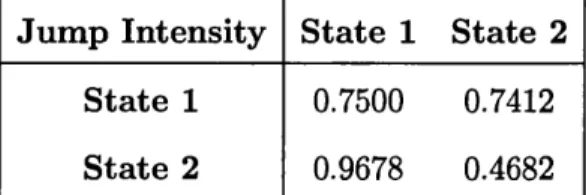
The interest rates for this model are ri = V2 = 0.03, and the risk-neutral

jump intensities are as shown in table 2.5.

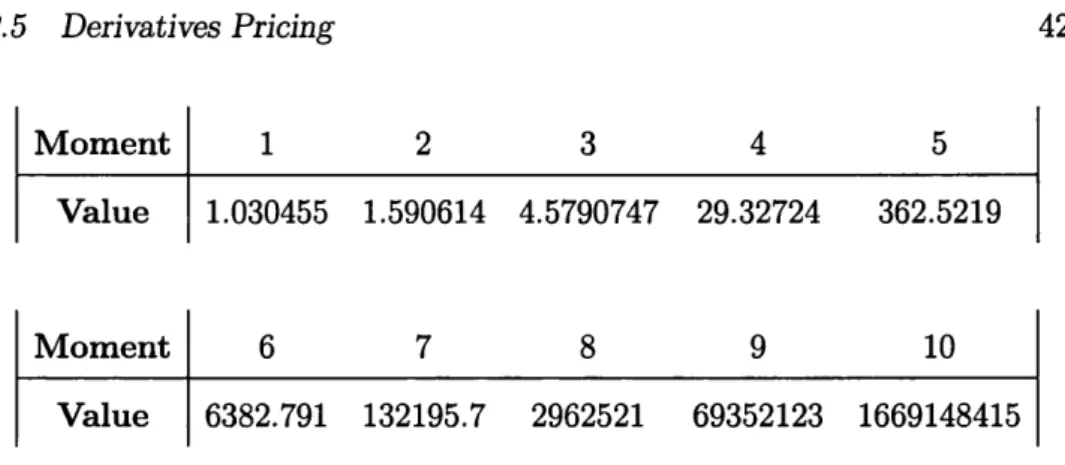
The moments of the price of this asset after a time of 1 year calculated

S ta te 1 S ta te 2

S ta te 1

S ta te 2

0.7500 0.7412

0.9678 0.4682

(57)

M o m e n t 1 2 3 4 5

V alue 1.030455 1.590614 4.5790747 29.32724 362.5219

M o m en t 6 7 8 9 1 0

V alue 6382.791 132195.7 2962521 69352123 1669148415

Table 2.6: Moments of price of asset 1 after 1 year starting in state 1.

using the above methodology, given that at time 0 we are in state 1, are

shown in table 2.6.

□

In order to price the derivative we need to calculate the expectation

EqI B ^ ^ Xt \J],

and for this in turn we will need to find the distribution of Si^r of which Xt

is a deterministic function. To this end, we will be able to use the moments

of Si^T to approximate its distribution^. In the following chapter we shall

compare methods of doing this with varying numbers of moments.

However, since and Si^r are both dependent of the path of the Markov

chain they will therefore be dependent, which means we will also need to

^Even though not every distribution may be uniquely determined by its moments (as

first shown by Hausdorff [1921]), nevertheless with any set of moments we are still able to

(58)

derive the distribution of conditional on Si^r- Rearranging (2.5.7) we

get

f /"T ^ 1

- I

Ju=Q

= exp { - I ^ l i v j d u

C I ft m

I J u=0

e x p { I " j=i

\

è

- è

6= 1 6= 1

and once again using corollary A.0.5 we can derive the moment-generating

function of conditional on St, and then too approximate its distribution.

We are now in a position to write the following:

C o ro lla ry 2.5.2. The price of a derivative on asset number i with time 0

price s, where the contingent claim is X { St) is given by

poo poo

c(o,s) = / / yX (z)fB -i^s,^{y)fs.,T{^)dydz

J y z = 0 J z = 0

where fn-^iSir distributions of the time T stock price

and the time T discout rate conditional on the stock price. When the interest

rate has constant value r in each state this simplifies to:

poo

c(0,s) = / X { z ) f s , ^ . j . { z ) d z . J z=0

(59)

Even though the above methodology is not of closed form, it does allow for

as much accuracy as required depending on how well we are able to approx

imate the distribution from its moments. How fast it will converge however

is a potential problem, as an obvious drawback of the above methodology is

the number of calculations th at need to be performed in order to calculate

the moments in equation (2.5.8), which as can be seen in corollary A.0.5 will

be large. So whether or not such calculations can be performed in reasonable

time will depend on the value of n, but more importantly the sizes of the

transition intensities and the duration T. Also, for the case where the in

terest rate r is dependent on the state, we have the undesirable requirement

th at the density function will need to be calculated for all values of

'S't.T-2.5.1

In terest-R ate D erivatives

We shall be considering more elaborate interest rate derivatives when we

look at Term-Structure Models in Chapter 4. However, within our current

framework we can calculate an explicit formula for a simple class of interest

rate derivatives.

Consider an asset with price Vt such th at

Vt = E

Bt _{— I- ^}2- ^ + . . . +Bt Bt

(60)

2.5 Derivatives Pricing 45

This payout represents th at of a coupon bond which pays h coupons of value

£ x i at time £ x2 at time Î2 and so on, where we have th at ti < Î2 < . .. <

th and th at t < t i. The final coupon at time th will normally also include the

nominal amount of the bond. The value of this bond is calculated by taking

the expectation of the sum of the discounted coupon payments to the current

time t. Let us denote the value of this bond given th at we are currently in

state j by . We therefore have

U=1

exp

- / ’. è

f c= l

I^Tkds ^ \ Yt = j (2.5.10)

Applying Taylor’s expansion to (2.5.10) we get

V i =

U=1 .y=o \

£ - / ; è

k=i

I ^ d s ] \ Y t = j

h ( o o / n \

=

j I

,

L y=0 \ k=l J )

(2.5.11)

where is defined in equation (1.3.6). For (2.5.11) to converge we require

th at

V «,*.

Even though (2.5.11) is not of closed form, it does allow for as much accuracy

(61)

We will now try to price a call option on this bond at time T where

ta < T < ta+i such that 0 < a < h and where to — t. The value of the bond

at time T will therefore be the expect discounted value of the remaining

h — a coupons. The strike price of this option is K , and we will denote the

discounted value of the option by Ct, so th at

where

3 = 1

4 = B tE [ B ^ ^ X T \Y t= j] ,

(2.5.12)

(2.5.13)

as well as

and

j=l

= max[Vÿ — K^O].

Applying Itô ’s lemma to (2.5.12), we find

dCt = B r ^ ' £ i i

i=i fe=l

dt. (2.5.14)

(62)

to be equal to zero, so that

fc= l

= (r, + cf A-"'

fc = l

for j = 1 ,... n, subject to = X ^ . Writing in matrix form, and noting th at

cj is now only a function of t and hence it is not necessary to use partial

derivatives, we therefore get th at

^

= (D (R ) - A , * ') c ,

with side condition

Cj- = Xj",

where A j and are defined in equations (2.3.7) and (2.3.8), and 1” is an

n x 1 column vector of I ’s. D (R ) once again represents the diagonal matrix

with the elements of R along the principal diagonal, where R has entries

R = {rj +

We can solve this to get

(63)

Chapter 3

N um erical M ethods for th e

Equity M odel

3.1

In tr o d u c tio n

In chapter 2 we looked at assets with price processes given by

j=l

iijdt + Y , + Ÿ ' f ' d N t

6=1 k=l

(3.1.1)

where we have state-dependent means and drifts fij and (j^j, and jump sizes

7-^^ when the model jumps from state j to state k. We saw in section 2.5

th at in order to price most derivatives of assets whose price processes fol

low this MCJD model, it is necessary to employ numerical methods. In this

chapter we shall look at various methods of doing this. We shall begin by

(64)

3.1 Introduction 49

trying to numerically solve the partial differential equations given in (2.5.4)

using finite-difference methods. We will then move on to consider paramet

ric methods to approximate the