Analysis of multivariate longitudinal categorical data subject to nonrandom missingness: a latent variable approach

(1)

Analysis of Multivariate Longitudinal

Categorical Data Subject to Nonrandom

Missingness: A Latent Variable Approach

Mai Sherif Hafez

A thesis submitted to the Department of Statistics of the London School of Economics for the degree of Doctor of Philosophy

(2)

Declaration

I certify that the thesis I have presented for examination for the PhD degree of the London School of Economics and Political Science is solely my own work other than where I have clearly indicated that it is the work of others (in which case the extent of any work carried out jointly by me and any other person is clearly identied in it).

The copyright of this thesis rests with the author. Quotation from it is permitted, provided that full acknowledgement is made. This thesis may not be reproduced without my prior written consent.

I warrant that this authorisation does not, to the best of my belief, infringe the rights of any third party.

I declare that my thesis consists of 33,615 words.

Statement of conjoint work:

(3)

Acknowledgements

First and foremost, I would like to express my sincere gratitude and appreciation to my supervisor, Professor Irini Moustaki for her continuous support, guidance and understanding and for making my Ph.D. a life-changing experience.

I am also thankful to Dr. Jouni Kuha, my advisor, for his valuable feedback and constructive recommendations during my studies.

My time at LSE was made enjoyable, thanks to the friendly and helpful sta and colleagues at the Department of Statistics of LSE. I particularly thank Ian Marshall for his genuine suppport.

I am both thankful and grateful to my loving parents, Mona and Sherif, and my supportive brother Kareem for their never-ending support and for always believing in me.

I am greatly indebted to my husband, Ismail, who made this experience possible by his undeniable sacrice and support even at the hardest of times, and to baby Amina who made the completion of this thesis a much bigger challenge.

(4)

Abstract

Longitudinal data are collected for studying changes across time. In social sciences, interest is often in theoretical constructs, such as attitudes, behaviour or abilities, which cannot be directly measured. In that case, multiple related manifest (observed) variables, for example survey questions or items in an ability test, are used as indicators for the constructs, which are themselves treated as latent (unobserved) variables. In this thesis, multivariate longitudinal data is considered where multiple observed variables, measured at each time point, are used as indicators for theoretical constructs (latent variables) of interest. The observed items and the latent variables are linked together via statistical latent variable models.

A common problem in longitudinal studies is missing data, where missingness can be classied into one of two forms. Dropout occurs when subjects exit the study prematurely, while intermittent missingness takes place when subjects miss one or more occasions but show up on a subsequent wave of the study. Ignor-ing the missIgnor-ingness mechanism can lead to biased estimates, especially when the missingness is nonrandom.

The approach proposed in this thesis uses latent variable models to capture the evolution of a latent phenomenon over time, while incorporating a missingness mechanism to account for possibly nonrandom forms of missingness. Two model specications are presented, the rst of which incorporates dropout only in the missingness mechanism, while the other accounts for both dropout and intermit-tent missingness allowing them to be informative by being modelled as functions of the latent variables and possibly observed covariates.

Models developed in this thesis consider ordinal and binary observed items, because such variables are often met in social surveys, while the underlying latent variables are assumed to be continuous.

(5)

List of Tables

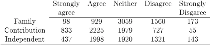
5.1 Frequency distribution for items (Family, Contribution and Inde-pendent) measured at rst wave . . . 82 5.2 Parameter estimates for Models 1 and 2, for modelling attitudes

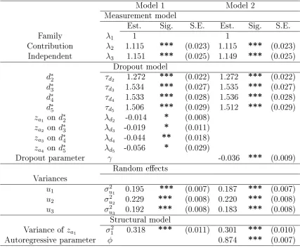
towards women's work from ve waves of the British Household Panel Survey . . . 85 5.3 Parameter estimates for regression of attitudinal latent variables on

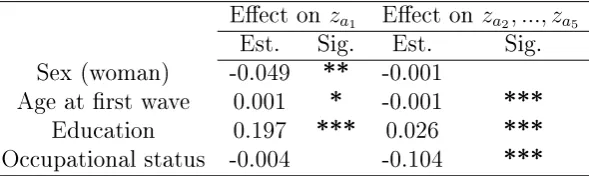
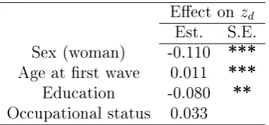
covariates (sex, age, education and occupational status) for Model 2 90 5.4 Parameter estimates for regression of the dropout latent variable on

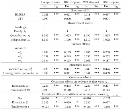
covariates (sex, age, education and occupational status) for Model 2 91 5.5 A sensitivity analysis for parameter estimates at four levels of dropout

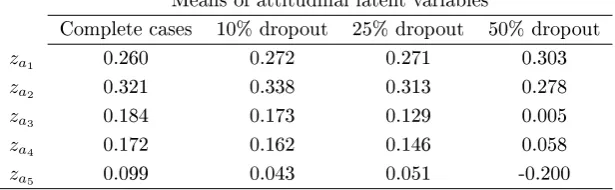
(0%, 10%, 25% and 50%) when dropouts are treated by listwise deletion . . . 94 5.6 Estimated means for attitudinal latent variables under four levels

of dropout (0%, 10%, 25% and 50%) when dropouts are treated by listwise deletion . . . 95 5.7 A sensitivity analysis for parameter estimates at four levels of dropout

(0%, 10%, 25% and 50%) when the dropout mechanism is ignored . 96 5.8 Estimated means for attitudinal latent variables under four levels

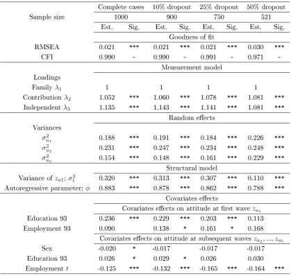
of dropout (0%, 10%, 25% and 50%) when the dropout mechanism is ignored . . . 97 5.9 A sensitivity analysis for parameter estimates at four levels of dropout

(0%, 10%, 25% and 50%) when the dropout mechanism is incorpo-rated . . . 98 5.10 A sensitivity analysis for covariates eects at four levels of dropout

(9)

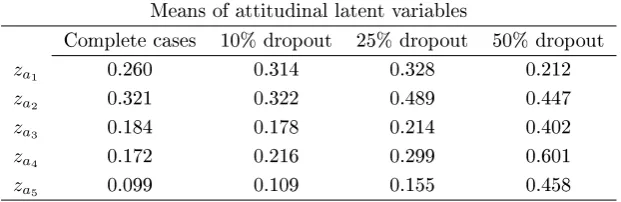
5.11 Estimated means for attitudinal latent variables under four levels of dropout (0%, 10%, 25% and 50%) when the dropout mechanism is incorporated . . . 100

6.1 Parameter estimates, standard errors and PSRF from MCMC after 10000 iterations for a model where attitude and covariates at rst wave aect probability of dropout; attitudes towards women's work data subject to dropout . . . 120 6.2 Parameter estimates, standard errors and PSRF from MCMC

af-ter 10000 iaf-terations for missingness mechanism in a model where attitude and covariates at rst wave aect probability of dropout, attitudes towards women's work data subject to dropout . . . 121

7.1 Parameter estimates, standard errors and PSRF from MCMC af-ter 10000 iaf-terations for a model where attitude at rst wave aects missingness; attitudes towards women's work data subject to inter-mittent missingness and dropout . . . 136 7.2 Parameter estimates, standard errors and PSRF from MCMC after

10000 iterations for missingness mechanism in a model where at-titude at rst wave aects missingness, atat-titudes towards women's work data subject to intermittent missingness and dropout . . . 137 7.3 Parameter estimates, standard errors and PSRF from MCMC after

4000 iterations for a model where time-dependent attitudes aect missingness; attitudes towards women's work data subject to inter-mittent missingness and dropout . . . 140 7.4 Parameter estimates, standard errors and PSRF from MCMC after

(10)

List of Figures

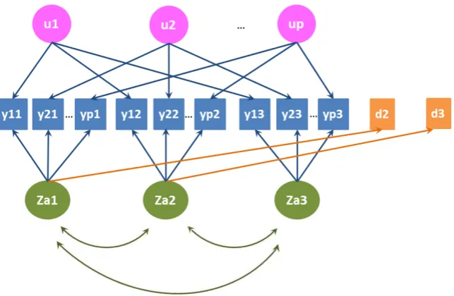
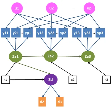
4.1 Path diagram for the rst model specication (Model 1). . . 75 4.2 Path diagram for the second model specication (Model 2), with

covariates. . . 77

6.1 Path diagram for a model where attitude at rst wave aects miss-ingness on all waves, an example with four time points . . . 106 6.2 Examples from WinBUGS manual showing: (top) multiple chains

for which convergence looks reasonable, (bottom) multiple chains which have not reached convergence . . . 113 6.3 Trace plots for a sample of parameters (intercepts, loadings,

regres-sion coecients and variances): (left) very well mixing of chains, (right) reasonable mixing of chains, attitudes towards women's work data subject to dropout . . . 118

7.1 Path diagram for a model where the time-dependent attitude aects missingness on the same wave, an example with four time points . . 131 7.2 Trace plots for a sample of parameters (intercepts, regression

(11)

Chapter 1

Introduction

In this thesis, we study latent variable modelling of multivariate longitudinal data subject to dierent types of missingness. Dropout and intermittent missingness are two types of missing data that we incorporate within a latent variable modelling framework to account for missingness while capturing the evolution of the latent phenomenon of interest.

(12)

items, because such variables are often met in social surveys, while we assume latent variables to be continuous.

Longitudinal data are collected for studying changes across time. Most of the existing research on longitudinal data focuses on repeated measures for one vari-able over time. Good starting points to the extensive literature on such univariate longitudinal data analysis are Diggle et al. (2013), who give a thorough overview of dierent methods, and Verbeke and Molenberghs (2000), who provide a compre-hensive treatment of linear mixed models for continuous longitudinal data. How-ever, when interest lies in how latent constructs change across time, the same multiple items are measured repeatedly at dierent time points, thus resulting in multivariate longitudinal data. Models for such data have been proposed by, for example, Fieuws and Verbeke (2004, 2006), Dunson (2003), and Cagnone et al. (2009), who model the associations of the latent and observed variables across time using random eects and/or latent variables.

Missing data is an unavoidable problem in almost every dataset, especially with longitudinal data. The most common type of missingness in longitudinal studies is dropout, where subjects exit the study prematurely. A crucial question for the analysis is whether or not those who drop out are systematically dierent from the ones who remain till the end of the study. Intermittent missingness where an individual misses an occasion and shows up on a subsequent wave, is also possible. In our research, these two types of missingness are incorporated within a latent variable model framework for multivariate longitudinal data.

(13)

theory (IRT) approach. Chapter 3 gives a review on missing data in general with a focus on existing methods for modelling univariate longitudinal data subject to dropout. A latent variable model for analysing multivariate ordinal longitudinal data subject to dropout is developed in Chapter 4 under the underlying variable approach, with two possible model specications. Chapter 5 provides an illustra-tion for the developed models by applying them to a real dataset about people's attitudes towards women's work from ve waves of the British Household Panel Survey (BHPS), along with a sensitivity analysis for dierent levels of dropout. In Chapter 6, one of the two model specications presented in Chapter 4 is used to develop a similar model for multivariate binary longitudinal data under IRT. Chapter 7 extends the model developed for binary observed items within an IRT framework to accommodate intermittent missingness together with dropout. Two possible specications are given for this model too. An application of this model is also presented using the British Household Panel Survey (BHPS) data. Chapter 8 gives a nal conclusion with highlights on the contribution of the research. Future areas for research are introduced including the incorporation of item non-response within the same model framework.

1.1 Notation

Observed variables will be denoted by y, where y will denote a (p×1) vector of

p observed variables. Observed variables will be either ordinal or binary. Latent

variables on the other hand will be denoted byz, wherezwill denote a(q×1)vector

of q latent variables. Latent variables are assumed to be normally distributed

(14)

The subscript i will be used to identify an observed variable y , while j will

be used to identify a latent variable variable z. Subscript for an individual of the

sample will be denoted bym.

(15)

Chapter 2

Literature Review on Latent

Variable Models

In order to develop a latent variable model for multivariate longitudinal data sub-ject to dierent forms of missingness, we rst need to review the existing literature on several topics. In this chapter, a literature review of latent variable models for multivariate complete data is given, rst in a cross-sectional context followed by the longitudinal case.

(16)

another main reason behind using latent variable models.

A latent variable model consists of two parts: a measurement part that links the observed variables to the latent variables; and a structural part that speci-es relationships among latent variablspeci-es and possibly covariatspeci-es. It is assumed that associations among observed variables are explained by the latent variables. This is an assumption of conditional independence where the observed items are independent given the latent variables.

Both manifest and latent variables can be either metric or categorical. Metric variables can be either discrete or continuous while categorical variables can be or-dered (ordinal) or unoror-dered (nominal). When both manifest and latent variables are metric, factor analysis is implemented. On the other hand, latent class analysis is applied when both manifest and latent variables are categorical. When manifest variables are categorical while latent variables are metric, latent trait analysis is the appropriate technique to adopt. Oppositely, when manifest variables are met-ric and latent variables are categomet-rical the suitable latent variable method is latent prole analysis. Bartholomew et al. (2011) present a unied approach for latent variable models for which each of the before-mentioned techniques can be viewed as a special case within the same general framework.

(17)

approach. Moustaki and Steele (2005) discuss a latent variable model with a mix-ture of categorical and survival items.

When the observed variables are categorical, there are two approaches for esti-mating parameters of the latent variable model. The underlying variable approach developed within the structural equation modelling (SEM) framework regards cat-egorical variables as manifestations of underlying unobserved continuous variables and thus the problem is converted into one with metric observed variables where factor analysis can be employed. The second approach is the response function approach, also known as item response theory (IRT) where distributional assump-tions are directly made on categorical manifest variables. A function is dened to give the probability of obtaining a response in each category of the categorical variable given the respondent's position on the latent variable scale.

In this thesis, we develop two types of models. The rst is for ordinal observed variables where the underlying variable approach is adopted. The second is for binary observed items in which the response function approach is employed. La-tent variables are assumed to be continuous in both cases. We therefore present the underlying variable approach for ordinal variables, followed by the item re-sponse theory for binary items. Bartholomew et al. (2011) (pp. 79-81) prove the equivalence of the two approaches for binary data.

2.1 The Underlying Variable Approach

(18)

between observed and latent variables on one hand (measurement model), and relationships among latent variables on the other (structural model).

Structural equation modelling is developed to handle continuous observed vari-ables. When observed variables are categorical, the underlying variable approach (UVA) is adopted. The underlying variable approach regards categorical variables as manifestations of underlying unobserved continuous variables and thus the prob-lem is converted into one with metric observed variables. Early contributions to the development of this method can be found in Jöreskog (1990, 1994), Muthén (1984) and Arminger and Küsters (1988) among others. The underlying variable approach is supported by software such as LISREL (Jöreskog and Sörbom (1996)) and Mplus (Muthén and Muthén (2011)).

Jöreskog (1990) denes an ordinal variable as one that takes values out of a set of ordered categories, such as a ve-category Likert scale. The categories are ordered ascendingly or descendingly but the distances between categories are nei-ther specied nor equal (example: strongly agree, agree, don't know, disagree and strongly disagree). Even when the categories of an ordinal variable are assigned numeric values, these values should not be treated as values of a continuous vari-able. Means, variances and covariances should not be calculated for an ordinal variable, but rather counts of responses in each category. That is why dierent techniques are applied when ordinal variables are used within structural equation models.

The underlying variable approach assumes that each ordinal variable y is a

manifestation of an underlying unobserved continuous variable y∗ which is used in

(19)

the relationship between these two variables is given in Jöreskog (2005) by

y=s ⇐⇒ τs−1 < y∗ < τs, s= 1,2, . . . , c, (2.1) where

−∞=τ0 < τ1 < τ2 < . . . < τc−1 < τc = +∞,

are parameters known as thresholds. There arec−1estimable thresholds for an

or-dinal variabley withccategories. It is the continuous unobserved variabley∗ that

is used in structural equation models not the ordinal observed variable y. Since

only ordinal information is available about the underlying continuous variable y∗,

its mean and variance are not identied and it is therefore assumed to have a stan-dard normal distribution with a density function φ(u)and a distribution function Φ(u). The choice of a standard normal distribution is explained in Jöreskog (2005)

by the fact that any continuous distribution can be transformed by a monotonic transformation into a standard normal. The probability of y falling in category s

can therefore be expressed by

πs = Pr [y=s] = Pr [τs−1 < y∗ < τs] =

ˆ τs

τs−1

φ(u)du= Φ(τs)−Φ(τs−1), and thus the threshold parameters are

τs = Φ−1(π1+π2+. . .+πs), s= 1, . . . , c−1,

(20)

(π1+π2+. . .+πs) is the probability that a response falls in category s or lower.

2.1.1 Measurement Model

The measurement model is the classical linear factor model

y_i∗ =αi+ q

X

j=1

λijzj+εi, i= 1, . . . , p, (2.2)

where αi is the mean of the ith item (here zero as the underlying variables are assumed to have a standard normal distribution), λij is the loading of the latent variablezj on the underlying continuous variabley∗i andεiis a normally distributed random error;εi ∼N(0, ωii2) that is uncorrelated with errors of other items. Or in matrix form

y∗ =α+Λz+,

whereαis a (p×1)vector of zero means, Λ is a(p×q)matrix of loadings, and is a (p×1)vector of normally distributed random errors ∼Np(0,Ω); such that

Ωis a (p×p) diagonal matrix of error variances.

Model (2.2) can also be referred to as a cumulative probit model or an ordered probit model (McElvey and Zavoina (1975)), an extension to the well-known probit model where the dependent variable is ordinal instead of binary. Alternatively, an ordered logit model, the counterpart of a logit model for modelling ordinal data, can be obtained by assuming a logistic distribution for the error termεi(McCullagh (1980)).

(21)

ordinal variableyi. This presentation will be introduced in Section 2.2 under item

response theory, with binary items as a special case.

The latent factors are assumed to account for dependencies among the ob-served variables (in this case the underlying variables); such that conditional on the latent factors, the observed variables are independent. If both the underlying continuous variables and the latent variables are assumed to have standard normal distributions, the conditional distribution of y∗ given z is

y∗ |z∼Np(Λz,Ω),

and the marginal distribution of y∗ is thus a multivariate normal

y∗ ∼Np(0,Σ),

whereΣ= ΛΛ0+ Ωis the theoretical covariance matrix of the underlying variables.

2.1.2 Structural Model

The structural part of the model which denes relationships among latent vari-ables, possibly in addition to a set of observed covariates xis given by

zj = q

X

l=1

φjlzl+ r

X

h=1

βjhxh+δj, j = 1, . . . , q,

(22)

error; δj ∼ N(0, υ2jj) that is uncorrelated with the latent factors zl. Or in matrix notation

z=Φz+βx+δ,

where Φ is a (q ×q) coecient matrix representing relationships among latent

variables, β is a (q×r) matrix of coecients representing dependence of latent

variables on covariates, and δ is a (q×1)vector of normally distributed random

errorsδ ∼Nq(0,Υ); such thatΥis a(q×q)covariance matrix of error terms that is possibly diagonal if the errors are not allowed to correlate.

2.1.3 Estimation

Estimation methods for the classical linear factor model, such as maximum likeli-hood (ML) and generalised least squares, provide parameter estimates that in some sense minimise the distance between the observed S and theoretical Σcovariance

matrices of the items. However, an observed covariance matrix cannot be obtained for categorical variables. Therefore, the estimation procedure should start in this case by obtaining a covariance/correlation matrix that can be employed in the estimation process.

(23)

es-timation of the model parameters is obtained. The third step involves eses-timation of the measurement/structural model parameters.

STEP 1: The probabilities πs are unknown population parameters and can be estimated by their corresponding sample quantities ps, which represent the

percentages of responses in category s. Therefore, the estimates of the thresholds

become

ˆ

τs = Φ−1(p1+p2+. . .+ps), s = 1, . . . , c−1,

where τˆs are the maximum likelihood estimators of τs based on the univariate marginal data.

STEP 2: Considering the bivariate distribution, suppose there are two ordinal variablesy1 and y2 withc1 and c2 categories, respectively. The bivariate marginal distribution can be represented by ac1×c2 contingency table that cross tabulates the two variables, such that the (s1, s2)th cell contains the counts ns1s2 of cases

in category s1 for the rst variable y1 and in category s2 for the second variable

y2. Since the underlying continuous variablesy₁∗ andy∗₂ are both standard normal,

their bivariate distribution is assumed to be standard bivariate normal with a correlation ρ12 (known as polychoric correlation). However this is an assumption to be tested as the normality ofy₁∗ and y∗₂ does not guarantee their joint bivariate

normality.

Let τ₁(1), τ₂(1), . . . , τ_c(1)

1−1 be thresholds for the underlying variable y

∗

1 and

τ₁(2), τ₂(2), . . . , τ_c(2)

2−1 be the corresponding thresholds for y

∗

(24)

the loglikelihood of the multinomial distribution,

lnL=

c1 X

s1=1

c2 X

s2=1

ns1s2logπs1s2(θ),

where

πs1s2(θ) = Pr [y1 =s1, y2 =s2] =

ˆ τs(1)₁

τ_s(1)

1−1

ˆ τs(2)₂

τ_s(2)

2−1

φ2(u, v)dudv,

such that

φ2(u, v) =

1 2πp(1−ρ2

12)

e− 1 2(1−ρ2₁₂)(u

2₋_2ρ

12uv+v2)

is the standard bivariate normal density with correlation ρ12. There are c1 ×c2 probabilitiesπs1s2(θ) that are functions of the parameter vector

θ = (τ₁(1), τ₂(1), . . . , τ_c(1)₁₋₁, τ₁(2), τ₂(2), . . . , τ_c(2)₂₋₁, ρ12). Maximising ln L is equivalent to minimising the bivariate t function

F(θ) =

c1 X

s1=1

c2 X

s2=1

ps1s2[ln ps1s2 −ln πs1s2(θ)] = X

s1s2

ps1s2ln[ps1s2/πs1s2(θ)],

where ps1s2 =ns1s2/N are the sample proportions.

A full information maximum likelihood estimation approach assumes a multi-variate normal distribution for all the underlying variables y₁∗, y∗₂, . . . , y_p∗.

Estima-tion involves minimising thep−dimensional t function over all response patterns

present in the data. This requires the evaluation of a p−dimensional integral for

(25)

-outlined above- is usually adopted.

STEP 3: Whereas Muthén (1984) uses a generalised least squares method for estimating parameters of the structural part of the model in the third step, Jöreskog (1990, 1994) uses a weighted least squares method where the weight matrix is an estimate of the inverse of the asymptotic covariance matrix of the polychoric correlations to estimate those parameters.

2.2 Item Response Theory Approach

The second approach for estimating parameters of a latent variable model with categorical manifest variables is the response function/item response theory (IRT) approach, where distributional assumptions are directly made on categorical man-ifest variables. A function is dened to give the probability of obtaining a re-sponse in each category of the categorical variable given the respondent's position on the latent variable scale. Within the response function framework, Moustaki (1996) develops a method for analysing latent variable models with metric and bi-nary manifest variables. Moustaki and Knott (2000a) propose a generalised linear model framework which allows simultaneous analysis for dierent types of manifest variables from the exponential family including metric, binary and nominal items. They dene a generalised linear model as a model of three components:

1. The random component: each manifest variable yi has a distribution from the exponential family with a canonical link function ηi taking the form

fi(yi, ηi, ϕi) = exp

yiηi−bi(ηi)

ϕi

+di(yi, ϕi)

(26)

wherebi(ηi)and di(yi, ϕi)take dierent forms depending on the distribution of the manifest variable yi, and ϕi is a scale parameter.

2. The systematic component: latent variables z1, ..., zq produce a linear pre-dictor ηi corresponding to each manifest variable yi as follows

ηi =αi+ q

X

j=1

λijzj, i= 1, ..., p.

3. The link function: it provides the link between the systematic component ηi and the conditional mean of the random component E(yi |z) such that

ηi =νi(µi(z)) =νi(E(yi |z)),

where the link functionνi can take diferent forms for dierent manifest vari-ables.

Binary variables are very common in social sciences. Even when responses fall in more than two categories, in many cases these are collapsed into just two whether the original categorical variable is ordinal or nominal. In this section, a model is outlined for binary manifest variables where latent variables are assumed to be continuous. For latent trait models with polytomous data, see for example; Bartholomew et al. (2011) and Moustaki and Knott (2000a).

2.2.1 A Measurement Model for Binary Manifest Variables

Let y = (y1, ..., yp)0 denote a vector of p binary manifest variables and z =

(27)

p. Possible responses to each binary variableyi, i= 1, . . . , pare coded as 0 or 1. A sensible assumption would be that the manifest binary variableyi has a Bernoulli distribution with expected value πi(z) = Pr (yi = 1 | z), which is a member of the exponential family thus taking the form of equation (2.3) with di(yi, ϕi) = 0 and ϕi = 1. An appropriate link function in the case of binary items is the logit function

ηi = logitπi(z) = αi+ q

X

j=1

λijzj, i= 1, . . . , p, (2.4)

whereαi is a constant term , andλij is the loading of the latent variablezj on the

ith binary item _yi. The intercept _α

i is known in educational testing, where this model originates, as the diculty parameter because increasing its value increases the probability of a positive response πi(z) = Pr (yi = 1 | z) for all respondents with dierent levels on the latent scale. The loadingλij is known as the discrimina-tion parameter because the larger its value, the easier it becomes to discriminate between two respondents at a given distance on the latent scale. This can be viewed as a logistic latent trait model with response function

πi(z) =

eαi+Pqj=1λijzj

1 +eαi+Pq_j₌₁λijzj.

An alternative model for binary responses uses the inverse of the normal dis-tribution function

Φ−1πi(z) = αi+ q

X

j=1

λijzj, i= 1, . . . , p,

(28)

extends to the case of ordinal items yi , but does not hold for unordered polyto-mous variables due to the fact that the categories are necessarily ordered in an underlying variable approach (Bartholomew et al. (2011)).

2.2.2 Structural Model

Latent variables are still assumed to be continuous. The structural part of the model is the same as that in a structural equation model outlined in Section 2.1.2.

2.2.3 Estimation

For a binary item yi, the conditional distribution of yi given z is taken to be the Bernoulli distribution,

gi(yi |z) = {πi(z)}yi{1−πi(z)}1−yi, yi = 0,1;i= 1, . . . , p, (2.5)

={1−πi(z)}exp{yi(αi+ q

X

j=1

λijzj)}.

Since only ycan be observed, Bartholomew et al. (2011) dene the joint

distribu-tion density funcdistribu-tion ofy by

f(y) =

ˆ

Rz

g(y|z)h(z)dz,

whereh(z)is the prior distribution ofz, andg(y|z)is the conditional distribution

of y given z. Our assumption is that of conditional independence, meaning that

if the set of latent variables zis complete, then zis sucient to explain all

depen-dencies among they's. In other words, conditioning onz, they's are independent.

(29)

of their marginal distributions, conditioning onz, as follows

g(y|z) =

p

Y

i=1

gi(yi |z), and thus f(y) can be written as

f(y) =

ˆ " _p Y

i=1

gi(yi |z) #

h(z)dz. (2.6)

Parameters of the model (αi andλijs) are estimated by maximum likelihood based on the joint distribution of the manifest variables given by equation (2.6). For a random sample of size n, the loglikelihood is written as

L=

n

X

m=1

logf(ym)

=

n

X

m=1

log

ˆ " _p Y

i=1

gi(yi |z) #

h(z)dz.

=

n

X

m=1

log

ˆ " _p Y

i=1

{1−πi(z)}exp{yi(αi+ q

X

j=1

λijzj)}

#

h(z)dz. (2.7)

(30)

EM algorithm explained in Moustaki and Knott (2000a). Alternatively, Bayesian estimation using Markov Chain Monte Carlo (MCMC) can be used (see Patz and Junker (999a, 1999b)).

2.3 Goodness-of-Fit

A latent variable model is accepted as a good t when the latent variables account for most of the associations among the observed variables. Testing whether the model provides a good t for the data involves comparing observed frequencies and estimates of expected frequencies under the model being tested. However, a global goodness-of-t measure that compares frequencies for full response patterns cannot be obtained under a limited information likelihood estimation approach that only estimates pairwise probabilities assuming underlying bivariate normality. Alternatively, instead of looking at whole response patterns, one may consider two-way margins. The likelihood ratio test statistic is given by

X_LR2 = 2

c1 X

s1=1

c2 X

s2=1

ns1s2ln[ps1s2/πˆs1s2] = 2N

c1 X

s1=1

c2 X

s2=1

ps1s2ln[ps1s2/πˆs1s2] = 2N F( ˆθ),

where_θˆ_{is the estimated parameter vector and}_π_ˆ

s1s2 =πs1s2( ˆθ).If the model holds,

the above statistic has an approximate chi-square distribution withc1c2−c1−c2 degrees of freedom (Jöreskog (2005)). By adding up all univariate and bivariate

X_{LRs, an overall likelihood ratio statistic is obtained. The alternative goodness-}2

of-t statistic

X_GF2 =

c1 X

s1=1

c2 X

s2=1

[(ns1s2 −Nˆπs1s2)

2

/(Nπˆs1s2)] =N

c1 X

s1=1

c2 X

s2=1

(ps1s2 −πˆs1s2)

2

(31)

has the same asymptotic distribution as X2

LR when the t is good.

Likelihood ratio and goodness-of-t tests can be greatly distorted in cases of sparseness in contingency tables leading to unreliable estimates, especially for bi-nary variables (Jöreskog (2005)). The test statistics are sensitive to sample sizes too. Large sample sizes lead to large values thus rejecting models even if the dif-ference between the sample and tted covariance matrices is small. On the other hand, small sample sizes lead to small values thus failing to reject the model due to lack of evidence.

The Root Mean Squared Error of Approximation (RMSEA) is a more robust measure, rst introduced by Steiger (1990), that is based on the non-central chi-square distribution and tests whether the model holds approximately. Values of thr RMSEA greater than 0.1 are indications of poor t. One advantage of the RMSEA is that it is usually reported with a condence interval. The Comparative Fit Index (CFI) is another t index, proposed by Bentler (1990), that compares the sample covariance matrix to a null model that assumes all latent variables are uncorrelated. Values of the CFI range between 0.0 and 1.0, with values closer to 1.0 indicating good t. Hooper et al. (2008) provide a list of available t indices for structural equation modelling in the literature, along with guidelines on their use.

(32)

For category s of variable i , the LR and GF-ts are dened as

LR−f it(i)_s = 2np(i)_s ln (p(i)_s /πˆ_s(i)),

GF −f it(i)_s =n(p(i)_s −πˆ_s(i))2/πˆ_s(i).

Summing these over s gives the univariate LR- and GF-Fits for variable i.

Simi-larly, the bivariate LR and GF-ts for categorys1 of variable iand category s2 of variable i0 are dened as

LR−f it(ii_s₁_s0)₂ = 2np(ii_s₁_s0)₂ln (p(ii_s₁_s0)₂/πˆ(ii_s₁_s0)₂),

GF −f it(ii_s₁_s0)₂ =n(p(ii_s₁_s0)₂ −πˆ(ii_s₁_s0)₂)2/πˆ_s(ii₁_s0₂).

Summing over s1 and s2 gives the bivariate LR and GF-ts for variables i and

i0. Since each of these t measures is based on a dierent contingency table with

a dierent number of cells, they are divided by the number of cells to allow for comparison across variables and pairs of variables. The overall t measure is the average of all pairwise t measures. Jöreskog and Moustaki (2001) suggest consid-ering a value larger than 4 to indicate a poor t. Cells with large contributions to the LR or GF-statistics will be nominated as the source of bad t. Bartholomew and Tzamourani (1999) propose alternative ways for assessing the goodness-of-t of this model based on Monte Carlo methods and residual analysis.

(33)

goodness-of-t tests. Akaike Information Criterion (AIC) takes into account both the value of the likelihood at the maximum likelihood solution and the number of estimated parameters

AIC =−2[maxL] + 2m,

where m is the number of estimated parameters. AIC can be used to compare

models with dierent numbers of latent factors, where the model with the smallest AIC is taken to be the best.

2.4 Latent Variable Models for Multivariate

Lon-gitudinal Data

When a single variable is measured repeatedly over time, the data is said to be longitudinal. Modelling univariate longitudinal data will be discussed briey in Chapter 3. However, when interest lies in capturing the evolution of a latent construct over time, latent variable models are used. The latent variables are measured via a number of observed items at each time point. When dealing with such models, there are two types of relationships to account for; those between dierent items within the same time point and those between the same items at dierent time points. At a given time, one or more latent variables can be used to account for dependencies among items, as outlined earlier in this chapter for cross-sectional data. The structural part of the model in this case addresses the question: how should the latent variables be linked in order to capture the longitudinal nature of the data?

(34)

multivariate ordinal longitudinal data where measurement invariance is assumed by setting thresholds and loadings of the same items to be equal over time. De-pendence among latent constructs over time is captured by regressing a latent variable on the same latent variable measured at a preceding time point. Mea-surement errors for the same items are correlated over time to account for their repitition.

(35)

Chapter 3

Missing Data: Review of Literature

Standard statistical techniques are designed to analyse complete datasets. They are developed under the assumption that the values for all variables recorded for all observations in the dataset are present. In practice, this is not usually the case. It is very often when dealing with a real dataset that some of the values are missing.

There are dierent types of missing data. Unit non-response is a severe type of missingness where data for an observation is completely missing, and thus no information can be inferred about this observation. Item non-response is another type of missing data where data for a respondent is collected for some variables but is missing for others. Intermittent missingness and dropout are two types of missingness specic to longitudinal data. Intermittent missingness occurs when a subject misses one or more occasions of a longitudinal study, but shows up on subsequent waves. Dropout is a more common type of missingness in longitudinal studies where subjects exit the study prematurely.

(36)

fol-lowed by a review of how dropout is treated in longitudinal studies.

3.1 Missingness in Cross-sectional Data

Rubin (1976) and Little and Rubin (2002) classify missing data into:

1. Data Missing Completely At Random (MCAR) where missingness is inde-pendent of both observed and unobserved data.

2. Data Missing At Random (MAR) such that missingness depends on the observed data, but is independent of the unobserved.

3. Data Missing Not At Random (MNAR) where missingness depends on the unobserved data, and possibly the observed data as well.

When data is missing completely at random (MCAR), it is reasonable to think of the observed data as a random subset of the complete data. If data is missing at random (MAR), it can still be viewed as a random subset dened for dierent values of the observed data. In these cases, the missingness mechanism is said to be ignorable. For the case when data is missing not at random (MNAR), the miss-ingness depends on the missing value itself and possibly on observed outcomes too, hence it is said that the missingness mechanism is non-ignorable or informative.

(37)

respondents with higher income are more likely than those with lower income to have missing data on income (Allison (2012)).

There are various ways in the literature for dealing with missing values, the simplest of which is complete-case analysis; also known as listwise deletion in which incompletely recorded units are discarded and a case is included in the analysis only if it is fully observed on all variables. Simplicity is the main advantage of this method. However, it can involve a great loss of information since values of a certain variable are discarded when they belong to cases that are missing for other variables. It can thus lead to serious biases and is not ecient except when the data is MCAR. Available-case analysis is a possible alternative for complete-case analysis that includes all complete-cases where the variable of interest is recorded, thus making use of all available information when making inference on a single variable. The main limitation of this method is that the sample base is not the same from one variable to another. This variability can cause practical problems and does not allow for comparability across variables if the missingness mechanism is not MCAR. A natural extension to accommodate meausures of covariation is pairwise deletion, in which a case remains in the analysis if the pair of variables being referenced have complete data for that case.

Weighting procedures for missing data use weights for observed units in an attempt to adjust for bias. This is a relatively simple device for reducing bias from complete-case analysis by yielding the same weight for all variables measured for each case. On the other hand, this simplicity entails a cost, in that weighting generally involves an increase in variance and is thus inecient (Little and Rubin (2002)).

(38)

with one of several options and analysis is carried out with the imputed data as if the dataset was completely observed (Little and Rubin (2002)). Single imputation can be applied to impute one value for each missing item. Options for imputation include unconditional or conditional mean imputation, where means from observed values of a variable or conditional means given data observed on other variables are substituted respectively; imputation by regression, where the missing variables for a unit are estimated by predicted values from the regression on the known variables for that unit; and hot deck imputation, where recorded units in the sample are used to substitute missing values. An important drawback of single imputation methods is that they do not account for imputation uncertainty and thus standard variance formulas applied to the imputed data systematically underestimate the variance of estimates, even if the model used to generate the imputations is correct.

Multiple Imputation (MI) has the added bonus of largely correcting this dis-advantage by imputing each missing value by more than one value, allowing for appropriate assessment of imputation uncertainty and increasing the eciency of estimates compared to those obtained from single imputation. MI was rst intro-duced by Rubin (1978) and keynote references include Rubin (1987) and Rubin (1996). When MI is implemented, each missing value is replaced by a vector of D

imputed values. Replacing each missing value by the rst component in its vector of imputations creates the rst completed data set, replacing each missing value by the second component in its vector creates the second completed data set, and so on. Standard complete-data methods are then used to analyse each of the D

imputed data sets. The Dsets of imputations can be viewed as repeated random

(39)

model for non-response. In that case, theD complete-data inferences can be

com-bined to form one inference that properly reects uncertainty due to missingness under that model, where the standard error adjusted for imputation accounts both for variation within and between imputed sets. When imputations are from two or more models for non-response, the combined inferences under the models can be contrasted across models to display the sensitivity of inference to models for non-response. MI provides statistically valid estimates, unilke simple ad hoc methods for handling missing data such as complete-case analysis, available-case analysis or mean imputation which only return valid estimates under the assumption that data is MCAR (Rubin (1996)).

A dierent approach for handling missing data is to rely on model-based pro-cedures in which a model is dened for missingness. Inference is then made on the likelihood dened under that model. A brief review of likelihood-based estimation for data with missingness is given below.

3.1.1 Likelihood-Based Estimation for Data With Missing

Values

Little and Rubin (2002) present a likelihood-based estimation method for data with missing values. Let y denote the complete data with no missing values such

that y can be written as y = (yobs, ymis) where yobs denotes the observed values and ymis denotes the missing values. The probability density function of y with a scalar or vector parameter θ; f(y | θ), can be written as a joint distribution of

(40)

f(yobs |θ) =

ˆ

f(yobs, ymis |θ)dymis. (3.1)

The missingness mechanism can be incorporated in the model by introducing an indicator random variable for missingness. For the ith variable of the mth

observation, an indicator random variable rmi is dened as

rmi =



  

  

1, ymi observed,

0, ymi missing.

The joint distribution of y and r, a (p×1) vector of missingness indicators, can

be written as

f(y, r |θ, ψ) = f(y|θ)f(r|y, ψ),

where f(r | y, ψ) is the distribution of the missingness mechanism and ψ is an

unknown parameter related to the missingness process. What is actually observed is values for yobs and r. To obtain the distribution of (yobs, r), we integrate out

ymis from the joint distribution of y= (yobs, ymis) and r:

f(yobs, r|θ, ψ) =

ˆ

f(yobs, ymis |θ)f(r |yobs,ymis, ψ)dymis. (3.2)

When the missingness mechanism does not depend on the missing valuesymis;

that is to say data is MAR, f(r| yobs, ymis, ψ) =f(r |yobs, ψ), and equation (3.2) can be written as

f(yobs, r|θ, ψ) =f(r|yobs,, ψ)

ˆ

(41)

=f(r |yobs, ψ)f(yobs |θ).

In some cases, the parameters θ and ψ are said to be distinct in the sense that

their joint parameter space is the product of the parameter space of θ and that of

ψ. In this case, the likelihood-based inferences for θ from the likelihood L(θ, ψ | yobs, r) =f(yobs, r|θ, ψ) is the same as that from the simplerL(θ |yobs) = f(yobs |

θ). That is, if the data is MAR (missingness does not depend on the missing

values), and the parameters θ and ψ are distinct, the missingness mechanism is

ignorable when inferences are made about θ. Inferences can then be based on

equation (3.1) rather than (3.2). However, it is not always easy to justify the assumption of random missingness. See Little and Rubin (2002) and Verbeke and Molenberghs (2000) for details.

The procedure for maximum likelihood estimation of parameters of an incom-plete dataset will be the same as that of a comincom-plete dataset with the dierence that it is based on the observed part of the data. The likelihood function is de-rived, and the ML estimates are obtained by solving the likelihood equations. The following are three available approaches to ML estimation with missing data.

3.1.1.1 Factoring the Likelihood

Assuming the missing-data mechanism is ignorable, the loglikelihood l(θ | yobs) =

logf(yobs |θ) based on the incomplete data may be rewritten as

(42)

where φ is a one-to-one monotone function of θ and φ1, φ2, ..., φJ are distinct pa-rameters (Little and Rubin (2002)). If this decomposition can be found, l(φ|yobs) can be maximised by maximisinglj(φj |yobs)separately. This is done by factoring the likelihood into functions that depend on distinct φj's. However, this

factori-sation does not always exist. Moreover, it can even exist but with non-distinct parameters φj's; and thus maximising the factors separately does not maximise

the likelihood.

3.1.1.2 Direct ML

Assuming the data is MAR (missingness mechanism is ignorable), ML estimates can be found by solving the score function

S(θ |yobs) =

∂l(θ |yobs)

∂θ = 0.

If a closed-form solution can be found for the above equation, ML estimates are obtained directly. If no closed-form solution can be attained, iterative methods are used to obtain the ML estimates. Some of these iterative methods, such as the Newton-Raphson algorithm, require calculating second derivatives of θ which can

become rather complicated.

3.1.1.3 The EM Algorithm

The Expectation-Maximisation (EM) algorithm, rst introduced by (Dempster et al. (1977)), is an iterative algorithm for ML estimation. It consists of two steps: the E-step which nds the conditional expectation of the loglikelihood l(θ |y)- or

(43)

data and the current estimate of the parameter θ, say θ(t)

E l(θ |y)|yobs, θ=θ(t)

=

ˆ

l(θ |y)f(ymis |yobs, θ=θ(t))dymis,

and the M-step which maximises this expected loglikelihood thus determining the new parameter θ(t+1). The new estimated parameter is substituted back in the

E-step and the above steps are repeated until convergence is attained. The expec-tations calculated in each step involve estimating functions of the missing dataymis which are then used to re-estimate the parameters. The new parameters are used to re-estimate functions of the missing values, and so on. Here data are assumed to be MAR, but in case the missingness is not at random, a factor representing the missing-data mechanism has to be included in the model. See examples for clarication in Little and Rubin (2002).

Bayesian Estimation

The likelihood function also plays a central role in Bayesian inference. In the Bayesian approach, parameters θ are treated as random variables rather than

xed quantities, and uncertainty about them is quantied using probability distri-butions. A parameter θ is assigned a prior distribution h(θ), and inference about

θ after observing the data y is based on its posterior distribution h(θ | y), which

is given by Bayes' theorem as:

h(θ|y) = h(θ)L(y|θ)

f(y) .

Point estimates of θ can be obtained as measures of the center of the posterior

(44)

and likelihood inference in case of large samples, and point out that Bayesian estimates correspond to ML estimates of θ when the prior distribution is uniform.

Furthermore, they highlight that in principle there is no dierence between ML or Bayes inference for incomplete data and ML or Bayes inference for complete data. The likelihood for the parameters based on the incomplete data is derived, ML estimates are found by solving the likelihood equation,while in case of Bayesian inference the posterior distribution is obtained by incorporating a prior distribution and performing the necessary integrations. More on Bayesian estimation is given in Chapter 6.

(45)

MI is used include cases such as: when the analysis model contains variables that were not included in the imputation model, and when the analysis model contains interactions and non-linearities, but the imputation model is strictly linear, and so on... Another point is that ML is more ecient than MI, where in case of MI full eciency requires an innite number of data sets to be analysed, which is not possible. Moreover, for a given set of data, ML always produces the same result, while MI gives a dierent result every time it is implemented. This partic-ular drawback of MI can be overcome by increasing the number of imputed data sets. On comparing ve methods (mean imputation, regression imputation, MI, EM and ML) for dealing with missing data in SEM with respect to the percent of bias in estimating parameters, Olinsky et al. (2003) nd ML to be superior in the estimation of most dierent types of parameters, followed by MI which is found superior in estimating standard errors but suers with increasing percentage of missing data.

3.1.2 Models for Data Missing Not At Random (MNAR)

So far, data has been assumed to be MAR. However, when the missingness is non-ignorable, the missingness mechanism should be incorporated in the model as in equation (3.2). There are two cases when missing data is non-ignorable:

1. The missing data mechanism is non-ignorable but known. The conditional distribution of r giveny= (yobs, ymis)depends on ymis, but does not depend on unknown parameters ψ.

(46)

known censoring point c, so that only values less than c are recorded. The

missingness mechanism is given by

f(r |y, ψ) =

n

Y

m=1

f(rm |ym, ψ),

where only n0 respondents are observed; rm = 1, m = 1, ..., n0 and rm =

0, m=n0+ 1, ..., n. Hence, f(rm |ym, ψ) =

      

1, rm = 1 andym < c, orrm = 0 andym ≥c,

0, otherwise,

This leads to a likelihood function involving an exponential distribution that depends on the known censoring pointc, but not on unknown parameters ψ

dening the missingness process:

f(yobs, r|θ) = n0

Y

m=1

f(ym, rm |θ) n

Y

m=n0₊₁

f(rm |θ)

=

n0

Y

m=1

f(ym |θ) Pr (ym < c|ym) n

Y

m=n0₊₁

Pr (ym ≥c|θ)

=θ−n0exp − n0 X

m=1

ym θ

!

exp

−(n−n

0₎_c

θ

,

since Pr (ym < c | ym) = 1 for respondents and Pr (ym ≥ c| θ) = exp −c_θ

for non-respondents, using properties of the exponential distribution.

(47)

practice, most non-ignorable missing data mechanisms will also be unknown as non-reponse will usually be related in some unknown way to the missing values even after adjusting for covariates known for both respondents and non-respondents.

Although the more general MNAR assumption explicitly incorporates the missing-ness mechanism, inferences produced are based on untestable assumptions about the distribution of the unobserved data given the observed. Methods involving non-ignorable missing data should always be viewed as part of a sensitivity anal-ysis in which the consequences of dierent modelling assumptions are explored (Little and Rubin (2002)).

3.2 Missingness in Longitudinal Data

In this section, we rst look at how longitudinal data is modelled, has the data been fully observed. Then, we review models for longitudinal data subject to dropout, the most common form of missing data in longitudinal studies.

3.2.1 Modelling Complete Univariate Longitudinal Data

(48)

For an individual m, longitudinal data is modelled using general linear

mixed-eects models (see for example Verbeke and Molenberghs (2000), Diggle et al. (2013) and Molenberghs and Verbeke (2001)) of the form

ym =Xmβ+Wmbm+εm, m = 1, . . . , n; (3.3) where ym = (ym1, ym2, ..., ymTm)

0 _{is a vector of all repeated measurements for the}

mth subject at Tm occasions, Xm is a (Tm×r1) matrix of known covariates, β is an(r1×1)vector of corresponding regression parameters (xed eects), Wm is a

(Tm×r2)matrix of subject-specic covariates that usually includes time as a covari-ate modelling howym evolves over time, bm is an(r2×1)vector of subject-specic parameters (random eects) describing how the evolution of the mth subject

de-viates from the average evolution in the population, and εm is a (Tm×1) vector of residuals for the mth subject. This model assumes that the vector of repeated

measurements for each subject follows a linear regression with some population-specic parameters β and some subject-specic parameters bm.

It is also assumed that bm ∼ N(0,B), εm ∼ N(0, σ2ITm), and that bm and

εm are independent. Conditioning on the random eect bm, ym follows a normal distribution with mean Xmβ+Wmbm and covariance matrix Σm =σ2ITm. The

marginal density function ofym, which is given by

g(ym |Xm) =

ˆ

g(ym |Xm,bm)h(bm)dbm,

will have a normal distribution with mean vector Xmβ and covariance matrix

Vm =WmBW0m+ Σm where Σm =σ2Itm (Verbeke and Molenberghs (2000)).

(49)

correlation in equation (3.3):

ym =Xmβ+Wmbm+um+εm,

where um is assumed a normal distribution; N(0, σu2Hm). The serial covariance matrix Hm only depends on m through the number of observations Tm and the time points at which measurements are taken. The structure of the matrix Hm is determined through the autocorrelation function ρ(tm − t0m). This function decreases such thatρ(0) = 1 and ρ(t)→ ∞ast → ∞. In this case the covariance

matrix of the marginal distribution of ym becomes Vm =WmBW0m+ Σm, where

Σm =σ2ITm+σ

2

uHm combines the measurement errors and the serial components. Longitudinal data can be viewed as two-level data, where occasions are nested within subjects. Rabe-Hesketh and Skrondal (2012) present a comprehensive re-view of models for univariate longitudinal data within this context, including xed-eects models where unobserved between-subject heterogeneity is represented by xed subject-specic eects, random-eects models where unobserved between-subject heterogeneity is represented by between-subject-specic eects that vary randomly, and dynamic models where the response at a given occasion depends on previous or lagged responses. In practice, dierent disciplines adopt dierent modelling strategies for longitudinal data. A summary of some of the main modelling tech-niques for longitudinal data presented by Rabe-Hesketh and Skrondal (2012) is given below.

(50)

would be

ymt =β0+α1m+β1x1m+β2x2m+ (β3+α2m)x3m+εmt,

where α1m and α2m are xed subject-specic intercept and slope parameters, re-spectively, x1 and x2 are covariates having the same eect for all subjects, and

x3 is a covariate having a subject-specic eect. Fixed-eects models are used to

estimate average within-subject relationships between time-varying covariates and the response variable, where every subject acts as its own control..

Similarly, a random-eects model may include a subject-specic random in-tercept resulting in a random-inin-tercept model, or random coecient for some of the covariates resulting in a random-coecient model, or both. An example of a random-eects model would be

ymt=β0+ζ1m+β1x1m+β2x2m+ (β3+ζ2m)x3m+εmt,

(51)

Dynamic models, also known as lagged-response models, autoregressive-response models and Markov models, model the response variable as a function of the same variable at previous occasions. One of the most widely used dynamic models is the rst-order autoregressive model [AR(1)], where the response ym,t is regressed on the preceding responseym,t−1. An example of an [AR(1)] model is

ymt=β0+φym,t−1+β1x1m+β2x2m+β3x3m+εmt. (3.4) Conditional on covariates, residuals εmt are assumed to be uncorrelated. This model assumes that all the within-subject dependence is due to the lagged re-sponse. It is noted that a xed autoregressive parameter φ is used here. It is

appropriate to use such a model when occasions are equally spaced in time. Oth-erwise, it would seem unrealistic or unjustiable to assume that the lagged response has the same eect on the current response regardless of the time interval between them. The above model can be extended to have a time-dependent autoregressive parameter φt instead of φ, to accommodate unequal spacing in time. Another extension can combine a lagged-response model with a random (or xed) intercept as follows

(52)

(represented by the lagged responses). Dynamic models are very popular among economists.

3.2.2 Longitudinal Data Subject to Dropout

The problem of missing data is very common in longitudinal studies. A distinction should be made here between intermittent missing values where a subject has missing data at some of the waves of the study, and dropout or attrition where missing values are only followed by missing values (i.e. subjects exit the study prematurely and never come back).

(53)

is to use all available data for each subject for as long as they last, without further adjustment, thus justifying our choice of likelihood-based approaches to handling dropout. This approach is fully ecient when dropout is at random.

When modelling longitudinal data subject to dropout, the joint density func-tion of both the measurement and dropout processes is considered. Suppose dropout occurs at occasiontof a longitudinal study. If dropout neither depends on

observed history data nor on the currently unobserved value, then missingness is considered to be completely at random. However, if the probability of dropout de-pends on previously observed values, but not on the currently missing value, then dropout is considered to be at random. If dropout is at random (or completely at random), and the parameters of the dropout process are distinct from those of the measurement process (an assumption we make throughout), the dropout is said to be ignorable and a valid analysis can be based on a likelihood that ignores the dropout mechanism. However, it is not always easy to justify the assumption of random dropout. If dropping out depends on the unobserved value at time of dropout, data is MNAR as in that case the missingness depends on the missing value itself which implies a systematic dierence between respondents who remain in the study and those who drop out. For example, in a medical study, those drop-ping out may be those with a deteriorating health condition. Hence the dropout mechanism is non-ignorable and should be incorporated in the analysis of the data, as ignoring it may lead to biased estimates of the parameters of interest.

(54)

complete sequence. Since in case of dropout, rm is of the form(1, ...,1,0, ...,0),km is then given by

km = 1 + Tm

X

t=1

rmt.

3.2.2.1 Selection Models

Selection models factorise the joint density of the full dataf(ym, km|Xm,Wm, θ, ψ) into the product of the marginal density of the measurement process and the con-ditional density of the missingness mechanism given the measurement as follows

f(ym, km |Xm,Wm, θ, ψ) =f(ym |Xm,Wm, θ)f(km |ym,Xm, ψ).

It is possible to have additional covariates in the missingness model but this is suppressed from notation (Molenberghs and Verbeke (2001)). In their key paper on selection models for non-ignorable dropout, Diggle and Kenward (1994) combine a multivariate Gaussian linear model for the measurement process with a logistic dropout model. A general model for informative dropout in longitudinal data for which completely random and random dropouts are special cases is proposed, and an associated methodology for likelihood-based inference is developed. A linear mixed model of the form (3.3) is assumed to model the measurement process. Assuming that the rst measurement ym1 is obtained for every subject in the study, the model for the dropout process is based on a logistic regression for the probability of dropout at occasiont, given the subject was still in the study up to

(55)

The dropout process is thus modelled by a logistic linear model of the form

logit [gt(hmt, ymt)] = logit [Pr (km =t |km >t, ym)] = ˜hmtΨ+ψ1ymt

=ψ0+ψ1ymt+ t

X

l=2

ψlym,t+1−l, (3.6) where _h˜

mt is a suitable subset of hmt. If ψ1 = 0, the dropout process is random, since the dropout will depend only on history and not on ymt. In this case, the

measurement and dropout models can be tted separately. If ψ1 6= 0, the dropout is nonrandom, since the dropout will depend on ymt, and the measurement and

dropout models cannot be tted separately.

Suppressing the index m for a subject, let y∗ = (y₁∗, y∗₂, ..., y_T∗)T _{denote the} complete vector of measurements atT time points. Lety= (y1, y2, ..., yT)T denote the vector of observed measurements with missing values recorded as 0. Therefore, it can be said that

yt=



  

  

y_t∗, t= 1, ..., k−1,

0, t_>k,

where 2 ₆ k ₆ T identies the dropout time. Let f∗(y;β,φ) denote the joint

probability density function (pdf) ofy∗ which follows a multivariate normal

distri-bution: y ∼M V N{Xβ, V(t,φ)}, where V(t,φ) is a block diagonal matrix with

(56)

Also, letht= (y1, ..., yt−1)denote an observed sequence of measurements observed up to time t−1, andy_t∗ the value that would be observed at time tif the unit did

not drop out.

Let f_t∗(yt | h∗t;θ) denote the conditional univariate normal pdf of yt∗ given

(y1, ..., yt−1) =h∗t andft(yt |ht;θ)the conditional pdf ofytgiven(y1, ..., yt−1) = ht. It follows that

Pr (yt= 0 |ht, yt−1 = 0) = 1, (3.7)

Pr (yt = 0|ht, yt−1 6= 0) =

ˆ

pt(ht, yt;ψ)ft∗(yt|ht;θ)dyt (3.8) and, for yt 6= 0,

ft(yt|ht;θ,ψ) = {1−pt(ht;yt;ψ)}ft∗(yt|ht;θ). (3.9) The above equations determine the joint distribution of y. For a complete

sequencey= (y1, ..., yT), and supressing the dependence on the parameters θ and ψ,

f(y) =f₁∗(y1) T

Y

t=2

ft(yt|ht)

=f∗(y)

T

Y

t=2

(57)

f(y) =f₁∗(y1)

(_k₋₁ Y

t=2

ft(yt |ht)

)

Pr (yk= 0 |hk)

=f_k∗₋₁(yk−1)

(_k₋₁ Y

t=2

[1−pt(ht, yt)]

)

Pr (yk = 0|hk), (3.11) where f_k∗₋₁(yk−1₎ _{denotes the joint pdf of the rst} _k₋₁_{non-missing elements.}

The loglikelihood function forθandψbased on the observed data{ym :m= 1, ..., n} is given by Diggle and Kenward (1994) as

l(θ,ψ) =l1(θ) +l2(ψ) +l3(θ, ψ), (3.12)

where

l1(θ) = n

X

m=1

logf_m∗(ym),

l2(ψ) = n

X

m=1 k−1

X

t=2

log{1−pt(hmt, ymt)}, and

l3(θ, ψ) =

X

m:km≤T

log Pr (k =km |ym).

In case of random dropout, l3 reduces to depend only on ψ, and therefore likelihoods forθ and ψ can be maximised separately. It is recommended anyways to maximise l1 and (l2 +l3) separately assuming random dropout as a means of obtaining initial values for the full maximisation of l(θ,ψ). If random dropout

(58)

measure-ment process. However, the full likelihood is still needed for inferences about the conditional process Y |non−dropout.

The model outlined above, introduced by Diggle and Kenward (1994), for non-random dropout is used as basis for many articles to follow. Molenberghs et al. (1997) use the same framework to model dropout probabilities when the variable of interest is ordinal. This requires a dierent approach to modelling the response and to the resulting likelihood calculations. Jansen et al. (2006) also study non-Gaussian outcomes such as binary, categorical or count data. They consider both generalised linear mixed models, for which the parameters can be estimated using maximum likelihood, and marginal models estimated through generalised estimat-ing equations, which is a non-likelihood method and hence requires modication to be valid under MAR. Molenberghs and Verbeke (2001) provide a review on linear mixed models for continuous longitudinal data focusing on the problem of missing data within both selection models and pattern-mixture models.

Sensitivity Analysis Within Selection Models

When tting a nonrandom dropout model, both the impact of the assumed dis-tributional form and the impact one or a few inuential subjects may have on the model parameters, should be considered.

In their work, Verbeke et al. (2001) adopt the same model proposed by Diggle and Kenward (1994) with the following perturbed version of the dropout model

(59)

The dierence in this model is that the ψ1ms are not viewed as parameters but

rather as local, individual-specic perturbations around a null model. The null model is taken to be the MAR model corresponding to setting ψ1 = 0. Verbeke et al. (2001) state that When small perturbations in a specic ψ1m lead to rela-tively large dierences in the model parameters, it suggests that the subject is likely to drive the conclusions...Such an observation is important also for our approach because then the impact (e.g., from inuential subjects) on dropout model param-eters extends to all functions that include these dropout paramparam-eters...Therefore, inuence on measurement model parameters can arise not only from incomplete observations but also from complete ones. A similar model is studied in Steen et al. (2001) for incomplete longitudinal multivariate ordinal data.

3.2.2.2 Pattern-Mixture Models

Pattern-mixture models, introduced by Little (1993), represent an alternative to selection models. They factorise the joint density in the opposite way