Interactive Segmentation Algorithm Based on Improved Random Walk

2017 2nd International Conference on Information Technology and Management Engineering (ITME 2017) ISBN: 978-1-60595-415-8

Interactive Segmentation Algorithm Based on Improved Random Walk

Ning WANG

, Yang MIAO

and Ji MA

1

Beijing Institute of Astronautical Systems Engineering, China Academy of Launch Vehicle Technology, Beijing China, 100076

2

College of Mechanical Engineering and Applied Electronics Technology, Beijing University of Technology, Beijing China 100124

Keywords: Image segmentation, Random walk model, Watershed.

Abstract. Interactive segmentation algorithm has been paid more and more attention in the field of image segmentation. Random walk algorithm is a proposed interactive segmentation algorithm based on graph theory, this paper proposes an improved Random Walk algorithm, the algorithm is more real-time than the original algorithm, and also has good robustness. This method adds the new improved Watershed algorithm to pre segmentation processing, reconstruct the connected domain graph, and the segmentation function Gauss area using 2 norm entropy reduction as a function of energy, finally it was solved by Random Walk algorithm. This method is faster than the original algorithm, the accuracy is satisfactory, and can be used for multi-target segmentation which has good robustness to noise.

Introduction

Image segmentation is an important part in the field of computer vision. The traditional manual segmentation is a waste of time and easy to cause errors, has been unable to meet the growing demand for massive image segmentation. The efficiency of automatic segmentation is very high, but the result is not satisfactory. So interactive segmentation is attracting more and more attention.

At present, the main interactive segmentation algorithms are Magic Wind, Intelligent Scissor, live-wire, Level set, Graph cuts, etc. Another popular segmentation algorithm in recent years is Random Walk. The Random Walk algorithm is based on graph theory, which can solve the problem of N - D segmentation, and has good robustness, and has a unique advantage for weak boundary segmentation. This paper mainly based on the Random Walk segmentation algorithm has been improved, increased the watershed pretreatment process, and re build a new energy function model of weights, making the results more reasonable.

Preprocessing

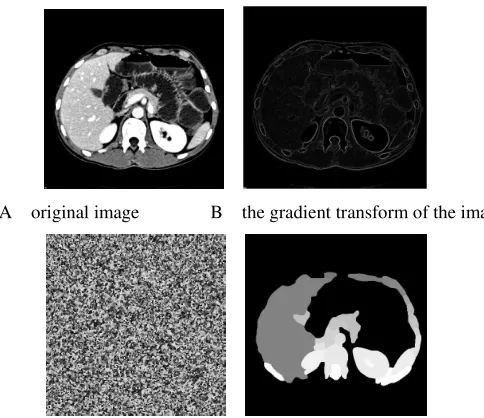
A original image B the gradient transform of the image

C Watershed segmentation without parameters D Threshold Watershed segmentation Figure 1. Watershed preprocessing.

The interactive segmentation algorithm described in this paper is as follows: [3]:

1) The gradient image of the original image is obtained by using the finite difference template. 2) The simulated rainfall model based on [2] is used to calculate the image after Watershed segmentation.

3) The adjacent connected graph is extracted and the relevant regional features are calculated. In this paper, the feature is the mean of the pixels in the image area after preprocessing.

4) Calculate the weights of the connection area, the weight calculation method as described in the 3.2 section of this article.

5) Mark the user input point.

6) Using Random Walk to solve the remaining non labeled regions, and calculate the probability that each region belongs to each marker. And according to the highest probability of the label of its segmentation.

7) According to the label of each region, the original pixel is calculated and the original image is segmented.

Walk Random Algorithm

Random Walk algorithm is the [4] algorithm based on graph theory, the algorithm derives from the problem that imitation drunk , walk to the randomness of each destination, while the reaction in mathematics is to construct a good picture, this picture on some nodes labeled nodes, each labeled as a destination, and the rest of the each node is regarded as a random walk, "the drunk", and the algorithm is the calculation of drawing other random walk to each marked point probability, so unlike the previous graph based methods such as Graph cuts, Lazy snapping, Grab Cut the rigid image two is divided into two categories, but can be more marked on the image, thus completing the multi object segmentation. For each node in the graph, there is a probability corresponding to each marker, and the sum of each point and the corresponding probability of each marker is 1. The probability of solving is transformed into solving a series of internal boundary conditions for the combination of Dirichlet problem.

Construct the Connection Diagram

ij

e . The figure in each edge is assigned a weight, the edge e_ij, the weight is w_ij, in order to explain the

probability of random walk selection w_ij >0. The provisions also assume that the graph is connected

with no direction.

Energy Function

According to the graph theory, the random walk model can be interpreted as follows: every node in the image corresponds to each node in the graph, and the weight of the edge in the graph is transformed according to the pixel value of the two points. Therefore, it is necessary to define a mapping function that specifies the conversion of the gray value to the weight. We choose the Gauss function which can maximize the entropy of the weight result [5].

2

exp( )

ij i j

w = −β g −g (1)

i

g represents the gray value of the image at the pixel i. This as a result of the pretreatment process of watershed, so a node in the graph represents a region of the image, we select pixels in the region as the mean pixel value of the node, the corresponding g_irepresent the region iaverage gray [6]. Energy

function of adjacent region:

2

exp( ( ) ( ) )

ij i j

w = −β D R −D R (2)

( ) i

i R i R g D R n

=

∑

β is the free parameter in the algorithm. It is found in the research that the 2 norm

2

i j ij

g −g ∀e ∈E of the gradient is normalized and the result of the formula (1) is better.

Graph Model Solution

The idea of the algorithm is to solve the problem by minimizing the following energy form:

2

1 1

[ ] ( )

2 _ij 2

T ij i j

e E

D x w x x x Lx

∈

=

∑

In Formula (4), Lis the Laplace matrix of the graph G, is defined as

( ) , if ,

, if ( ),

0, ij k N i

ij ij

w i j

L w j N i

otherwise ∈  =  − ∈   

∑

In this N i( ) is a set of index values of all adjacent nodes that contain the i node. The Laplasse matrix is symmetric and positive definite. With the appropriate boundary conditions, the solution to the problem corresponds to the probability that each node is different from each other. For K markers, K-1 only needs to solve a Dirichlet problem, finally a marking probability and other add up to 1. In order to be consistent with the boundary conditions, the nodes are divided into two complementary sets, one is the labeled set of nodes V_M, and the other is the set of nodes V_Uthat have not been

marked,V_M ∪V_U =V ,V_M ∩V_U = ∅ In order not to lose the generality, the nodes in theLandx

sequence are reordered, the marked nodes are arranged in front, and the marked nodes are arranged in the back, so the equation (2) can be decomposed into the following forms

1 [ ] [ ] 2 M M T T

U M U T

U U

x

L B

D x x x

B L x

 

 

=   =

   

1

( 2 )

2

T T T T

M M M U M U U U

Solving the differential x_Ufor equation [D x_U], the solution of the minimum value of the equation can be obtained

T

U U M

L x = −B x ₍₇₎

For any tag s, define a set of seed points ( )Q v_j =s,∀v_j∈V_M. Therefore, the probability vector of

the marked points is defined

1 if ( ) , 0 if ( ) ,

j s

j

j

Q v s m

Q v s

=



=

≠



(8)

Therefore, for marking s, solving combinatorial Dirichlet problem can be solved in the following matrix.

s T s

U

L x = −B m (9) The result is that the probability of each node for each tag. In this paper, we use the adjacent region graph constructed by watershed to calculate the results of the previous section, and obtain the solution of the matrix by using the conjugate gradient solver, and use ILU (incomplete LU) as the preprocessor. The Laplasse matrix is a sparse matrix, so the data storage is based on the compressed data storage format. Because beta is an empirical value, in the calculation, set to 45.

Experimental Result Analysis

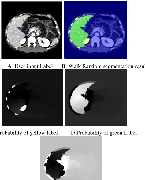
In this paper the following results are shown for a total of two sets of test images, the first group is a natural image, the image size for the second group is the medical image, the image size is. In the first group, we made a total of three sets of markers, the blue marked the background, the yellow mark is the flower leaf, green marker of the pot, the segmentation effect is satisfied. In the second group, the blue labeled ribs, the Yellow markers of the liver, and the green markers of the rest, also had fairly desirable segmentation results. The calculation time of the first image watershed time 63ms sparse matrix solver, the computation time is 40ms, the total processing time and the structure of the pro domain connection graph is not greater than 500ms, while no watershed treatment result is about 50s, second pictures of watershed time 93ms, sparse matrix for 170ms in total, the processing time is less than 700ms, while the processing time for watershed original random walk is about 80s. In Figure 2 and figure 3 for the segmentation results, and each token conversion probability graph, the graph and bright pixels in a pixel portion in the token under higher probability.

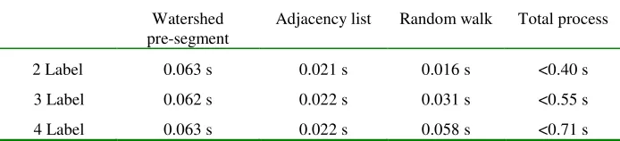
In order to obtain a general comprehensive evaluation for image database UC in Berkeley with the method of test equipment is 2.93G-Intel (R) Core (TM) PC 2 Duo CPU, memory 2G, operating system for 32 Window 7. The experimental data is composed of 4 selected images from the image library, each of which consists of 25 color images, each with a reference size of 481 x 321. There are a large number of manual segmentation images in the image library, so as to facilitate the segmentation of the image and the demarcation of the boundary. The average processing time for each step of the image is shown in table 1.

Table 1. The calculation time of each part of the algorithm. Watershed

pre-segment

Adjacency list Random walk Total process

2 Label 0.063 s 0.021 s 0.016 s <0.40 s

3 Label 0.062 s 0.022 s 0.031 s <0.55 s

4 Label 0.063 s 0.022 s 0.058 s <0.71 s

The comparison of the computational time of the proposed algorithm with the original Random Walk is compared in table 2.

A User input Label B Walk Random segmentation results

C Probability of yellow label D Probability of green Label

E Probability of blue Label

Figure 2. Natural image segmentation results.

A User input Label B Walk Random segmentation results

C Probability of yellow label D Probability of green Label

E Probability of blue Label

Table 2. Fine matching results. Random Walk raw

computing time

Calculation time of the algorithm

Contrast fast multiple

2 Label <29 s <0.40 s 72.5

3 Label <57 s <0.55 s 103.6

4 Label <75 s <0.71 s 105.6

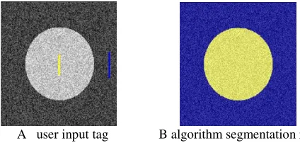
The data given in Table 2 shows that the speed of the algorithm is greatly improved compared with the original algorithm. The results can be applied in practice. At the same time, the algorithm has a strong robustness to noise image because of the segmentation based on morphology. As shown in Figure 4 for Gauss noise image segmentation results, it can be seen that the edge of the image segmentation is ideal.

A user input tag B algorithm segmentation results Figure 4. Gauss noise image segmentation results.

Summary

In this paper, the speed improvement of the improved algorithm based on multi objective interactive segmentation is studied. The experimental results show that the proposed algorithm can complete real-time image of the multi object segmentation, and has good robustness to the noise image, but the algorithm for target and background color similar segmentation is not particularly desirable, how to further improve the algorithm is the main target for image segmentation accuracy.

References

[1]Luc Vincent, Pierre Soille. Watersheds in Digital Spaces: An Efficient Algorithm Based on Immersion Simulations [J]. Image and Vision Computing, Pattern recognition and artificial intelligence, 1991, 13(6):583-598.

[2]Victor Osma-Ruiz, Juan I. Godino-Llorete, Nicolas Saenz-Lechon, Pedro Gomez-Vilda. An improved watershed algotithm based on efficient computation of shortest paths [J]. Pattern Recognition, 2007, 40:1074-1090.

[3]Christophe Chefd’hotel, Alexis Sebbane. Random Walk and Front Propagation on Watershed Adjacency Graph for Multilabel Image Segmentation [J]. In Proc. of Intl. Conf. on Computer Vision., Oct. 2007.

[4]Leo Grady. Random Walk for Image Segmentation [J]. Pattern recognition and artificial intelligence, 2006, 28(11):1-17.

[5]Leo Grady, Marie-Pierre Jolly. Weights and Topology: A Study of the Effects of Graph Construction on 3D Image Segmentation [J]. In Proc of Med Im Comp. & Comp Assisted Inter., 2008.