2016 International Conference on Manufacturing Science and Information Engineering (ICMSIE 2016) ISBN: 978-1-60595-325-0
Development of a Simulation Software for
Subway Train Traction and Braking Process
Based on Simulink and Lab VIEW
XIAODONG WANG, MENGLING WU and CHI LEI
ABSTRACT
The simulation software for subway train traction and braking process is composed of a GUI based on Lab VIEW and an underlying model based on Matlab/Simulink. An underlying model consists of a traction system model and a braking system model, which is used to achieve simulation of traction and braking process. A GUI of the software is mainly be used to input model parameters, display operation status and simulation data. This software integrates the simulation of traction and braking process which can simulate the real status of train and provides a reference for setting subway stations and route optimization. In addition, the simplification of traction model and braking model shortens the operation time of the software, so as to achieve a real-time simulation.1
INTRODUCTION
Studying of train traction and braking is of great significance to high-speed railway trains and urban rail transit. This paper simulates the traction and braking process by establishing a traction system model and braking system model, so as to research the process and status of train traction and braking. Compared with real vehicles’ online experiment, simulation the simulation method has the following distinct advantages: low cost, easy to operate and implement. Currently, Wenli Lin [1], Ruigang Song [2] have already built train traction system model, and Piechowiak [3,4] has already developed a simulation model of train braking system. But no one has established a model integrating the traction with braking process by far. This paper develops a simulation software for subway train traction and braking process based on Simulink and Lab VIEW, of which main features are: 1. The
1
software integrated the train traction with braking, which can simulate different conditions of traction and braking, and provides a reference for setting subway stations and route optimization meanwhile; 2. The software can simplify the train model so as to achieve a real-time simulation and keep the main parameters for the research of train traction and braking at the same time.
SOFTWARE CONFIGURATION AND PARAMETER CONFIGURATION
Brake System
Model Traction
System Model
GUI (LabVIEW)
[image:2.612.178.417.220.368.2]Underlying model(Matlab-Simulink) NI SIT
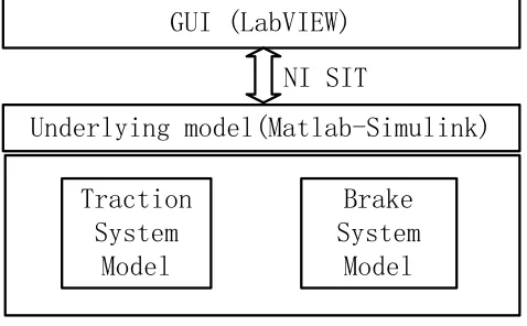
Figure 1. Configuration of the software.
The configuration of the software is shown in Figure 1. The whole software consists of a graphical user interface (GUI) and an underlying model. The underlying model is composed of attraction system model and a braking system model, which accomplish traction and braking under the control of GUI.
The GUI is a computer code based on Lab VIEW, and the underlying model is built based on Matlab-Simulink. A software interface, called Simulation Interface Toolkit (SIT), originally developed by the National Instruments (NI) Corporation, is used to facilitate the communication between the GUI and the underlying model.
The software is used to simulate the traction and braking process of a type of subway train. The subway train contains four motor cars and two trailer cars:
=Tc * Mp * M * M * Mp * Tc = (1)
Definitions: =,*:Coupler Tc: Trailer Car
Mp: Motor Car with Pantograph M: Motor Car
R=(16.18+0.2422V) Wm+(7.65+0.0275V)Wt+(0.275+0.0765(n-1))V2 (2)
Definitions:
R: Basic Operation Resistance Wm: Weight of Motor Car
V: Velocity
Wt: Weight of Trailer Car n: Number of Car
[image:3.612.180.415.229.329.2]The train load under different simulation conditions is shown in TABLEI.
TABLE I. TRAIN LOAD.
Tc1 Mp1 M1 M2 Mp2 Tc2
AW0 30 35 35 35 35 30
AW2 43.56 50.24 50.24 50.24 50.24 43.56
[image:3.612.190.406.369.470.2]AW3 47.4 54.5 54.5 54.5 54.5 47.4
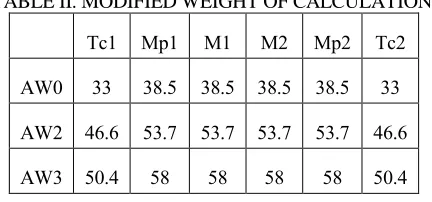
TABLE II. MODIFIED WEIGHT OF CALCULATION.
Tc1 Mp1 M1 M2 Mp2 Tc2
AW0 33 38.5 38.5 38.5 38.5 33
AW2 46.6 53.7 53.7 53.7 53.7 46.6
AW3 50.4 58 58 58 58 50.4
In traction and braking calculation, considering the inertia, the train load can't directly be used in the calculation. The train load must be modified as a weight of calculation. The formula is:
W'=L+ (W*n) (3)
Definitions:
W': Modified Weight of Calculation L: Load
W: Empty Vehicle Weight n: Inertial coefficient
TRACTION SYSTEM MODELING
Principle Of Traction Modeling
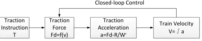
[image:4.612.177.423.303.477.2]The traction calculation model of urban rail transit vehicles can be divided into single-particle mode and multi-particle mode [5]. In order to achieve a real-time simulation, single-particle is selected as a simple modeling method. When the controller sends out the traction instruction, the traction control system obtains the traction force (Fd) in the current velocity from the traction characteristic curve (shown in Figure 2). Then the system calculates the traction acceleration (a) according to the calculation load of train (W') and the basic running resistance (R). According to the integral of the traction acceleration, the system gets the velocity of next moment(V). The closed-loop control based on velocity is completed. The control principle is shown in Figure 3.
Figure 2. Traction characteristic curve.
Traction Force Fd=f(v)
Traction Acceleration
a=Fd-R/W'
Traction Instruction
T
Train Velocity V=∫a Closed-loop Control
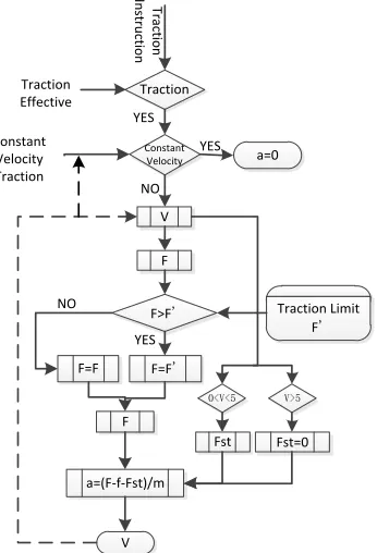
[image:4.612.133.464.545.613.2]Logic Of Traction Control
The software simulates the generation and transmission of the train traction instructions, and generates the corresponding traction force with implementation of the traction limit after the judgment of the starting state, traction effective and constant velocity traction. The logic of traction control is shown in Figure 4, and the specific functions are as follows:
TRACTION LEVEL
Traction level isn't step less, and there are totally ten traction levels. In the process of traction, the system treats the traction characteristic curve as the tenth traction state, and the rest of the traction levels state are linear interpolation from zero to the traction characteristic curve.
STARTING STATE
In order to simulate the train starting state as a real traction condition, the system is regarded as starting state when the train velocity is less than 5km/h. And the running resistance of the train is composed of the basic running resistance and the starting resistance. The starting resistance is 39.2N/t.
[image:5.612.217.390.385.639.2]Tr ac tio n In st ru ct io n Traction Constant Velocity YES a=0 YES F F>F' V F=F' Traction Limit F' YES F 0<V<5 V>5 V F=F NO NO a=(F-f-Fst)/m Fst=0 Fst Traction Effective Constant Velocity Traction
STATE OF CONSTANT VELOCITY
The system sets a constant velocity signal. When the signal is effective, the train runs with constant velocity. When the train velocity closes to be greater than 80km/h, the constant velocity signal becomes effective, and the train runs with constant velocity, in order to achieve the limit of maximum operating velocity.
COASTING STATE
The system sets a traction effective signal. When the signal is invalid or the traction level is zero, the train enters the coasting state.
TRACTION LIMIT
The system considers the traction limit. When the traction force is greater than the maximum traction limit, the traction force can't be increased anymore.
ADHESION LIMIT
According to the calculation under the normal rail condition, the maximum traction force can't be more than the maximum adhesion focus anytime. So the system doesn't consider the adhesion limit, and it always meets with adhesion condition.
BRAKING SYSTEM MODELING
Principle of Braking Modeling
Figure 5. Braking characteristic curve.
Traction Force Fd=f(v)
Traction Acceleration
a=Fd-R/W'
Traction Instruction
T
Train Velocity V=∫a Closed-loop Control
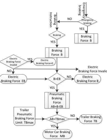
Em er ge n cy b ra kin g B ra kin g In st ru ct io n Electric Braking Force Invalid Braking
Braking Force B YES Electric Braking Force Invalid B>EB Electric
Braking Force EB NO Electric Braking Force=0 YES Pneumatic Braking Force AB=B-EB Trailer Pneumatic Braking Force
Limit TBmax AB>TBmax
Motor Car Braking Force MB
YES YES
Electric Braking Force B NO
Trailer Braking Force TB NO
Emergency braking
[image:8.612.184.406.89.379.2]Braking Force B YES NO
Figure 7. Logic of traction control.
Logic of Braking Control
The software simulates the generation and transmission of the train braking instructions, and can complete the function of service braking, emergency braking. And the system considers electro-pneumatic. The logic of braking control is shown in Figure 7, and the specific functions are as follow:
BRAKING LEVEL
Figure 8. The target deceleration of different levels in the velocity of 0~70km/h and 70~80km/h.
[image:9.612.171.423.300.655.2]ELECTRO-PNEUMATIC
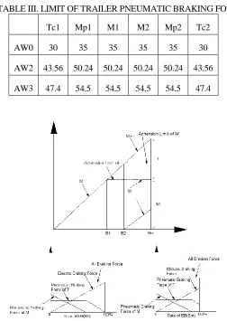
TABLE III. LIMIT OF TRAILER PNEUMATIC BRAKING FORCE.
Tc1 Mp1 M1 M2 Mp2 Tc2
AW0 30 35 35 35 35 30
AW2 43.56 50.24 50.24 50.24 50.24 43.56
When server braking or prompt braking applies, the system calculates the target deceleration according to the actual load, and compares it with the maximum electric braking force in the current velocity. If electric braking force isn't enough, the braking force will be supplemented by pneumatic braking force of trailer (two trailer equally) firstly. If braking force is still not enough (the limit of trailer pneumatic braking force is shown in TABLE III), it will be supplemented by pneumatic braking force of motor car (four motor car equally) secondly. Electro-pneumatic is shown in Figure 9.
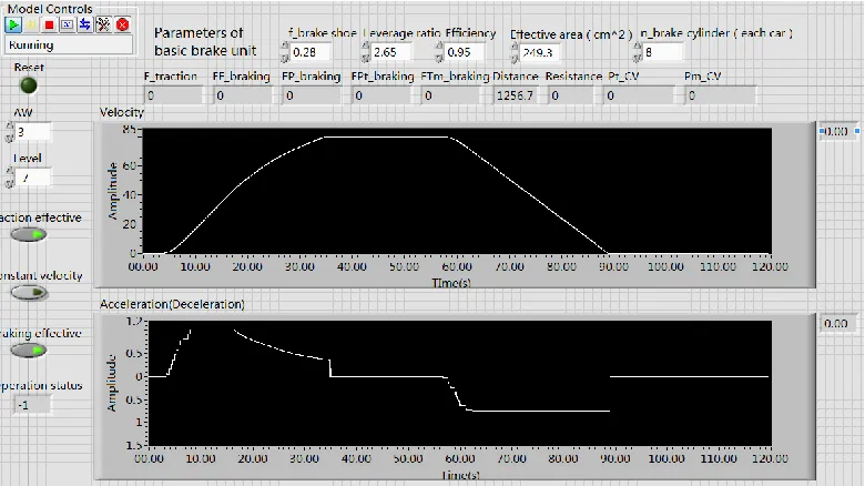
GRAPHICAL USER INTERFACE
A GUI designed by Lab VIEW computer code is to satisfy the following purposes:
Display of state: running state of software, train.
Setting parameters: chosen of working condition, chosen of level, displacement, the brake shoe friction coefficient, leverage ratio, efficiency, effective area, brake cylinder number, etc.
Drawing curve and display date: mainly draws the velocity-time curve and the acceleration-time curve; displays the traction force, the electric braking force, the pneumatic braking force, the trailer pneumatic brake force, the motor car pneumatic braking force, the running distance, the running resistance, the trailer CV pressure, the motor car CV pressure, etc.
Other functions: controls the effectiveness of traction or braking function, achieve the function of constant velocity operation.
Figure 10. The parameters configuration state and results of data.
CONCLUSION
The simulation software for subway train traction and braking process consists of GUI and underlying model. Underlying model is composed of a traction system model and a braking system model based on Matlab/Simulink, which is used to achieve simulation of traction and braking process. And the GUI of the software based on Lab VIEW is used to input model parameters, display operation status and simulation data.
The software, integrating the simulation of traction with braking, can simulate the actual state of the train operation, and provides a reference for the subway station setting and railway line optimization. In addition, the simplification of the traction model and the braking model can shorten the operation time of the software, so as to realize the function of real-time simulation.
ACKNOWLEDGMENT
REFERENCES
1. Wenli Lin. 2010. “Analysis Modeling and Optimization Of Metro Traction System”. Beijing Jiaotong University.
2. Ruigang Song, 2012. “Research on Modeling of Dynamic Tration Characteristics and Test System of Urban Rail Vehicles”. Journal Of The China Railway Society. 34(7), 0036-07.
3. Piechowiak,T.2009. “Pneumatic train brake simulation method”. Veh Syst Dyn, 47(12), 1473-92.
4. Piechowiak, T. 2010. “Verification of pneumatic railway brake models”. Veh Syst Dyn, 48(3), 283-99.
5. Baohua Mao. 2008. “Vehicle Calculation And Design”. China Communications Press. 6. Jun Chen. 2013. “Research on Electro-pneumatic blend Braking Technology of the
Subway rail trains”. Dalian Jiaotong University.
7. Lirong Qu, Rong Hu, Shoukang Fan. 2011. “Mixed Programming Technology of Labview and Matlab. Beijing”. China Machine Press.