ISSN: 1992-8645 www.jatit.org E-ISSN: 1817-3195
OPTIMIZATION ECONOMIC POWER GENERATION USING
MODIFIED IMPROVED PSO ALGORITHM METHODS
1STEVEN HUMENA,. 2SALAMA MANJANG,. 3 INDAR CHAERAH GUNADIN 1,
Electrical Engineering Student, Hasanuddin University, Indonesia
2,3,
Electrical Engineering Lecture, Hasanuddin University, Indonesia
E-mail: [email protected], [email protected], [email protected]
ABSTRACT
Fuel consumption on operation of power generation is one of the things that need to get special attention because most of the operating costs incurred is fuel costs. The output of the power generation always strived to meet the needs of the loads. Economical optimization is an attempt to minimize the cost of power generation fuel. This research proposes the application of the Algorithm Methods of Modified Improved Particle Swarm Optimization (MIPSO) that are compared with the Lagrange method and the Improved Particle Swarm Optimization (IPSO) in the case of the IEEE 30-bus system as a validation, in which the results of the simulation of MIPSO method can minimize the cost to 575.28 $/hour compared to the Lagrange method at 575.32 $/hour and IPSO method at 575.29 $ /hour. Then MIPSO Algorithm Method applied to the SULSELBAR 150 kV interconnection system are compared with the cost of a real system, the results of the simulation showed that the MIPSO method algorithm can reduce the cost of power plant to Rp. 51,706,000.- per hour or decrease operating costs of around 13.73% per hour.
Keywords: Optimization Economic, Modified Improved PSO Algorithm Methods, 150kv SULSELBAR Interconnection System
1. INTRODUCTION
The main role of the electrical power system is to ensure that the electrical energy needs of customers can be served. But in doing so, the operation of the interconnection of electric power systems usually have a common problem, namely how to produce maximum output power with minimum operation cost of generating electric energy. There fore, it is necessary to have a power flow optimization function which can minimize the cost of electric energy generation that is affected by changes in the energy needs within a specified time.
Optimization Economic is a procedure to determine the electrical power generated by the plant is connected to the system's electrical interconnection so that the overall cost of operation isminimized simultaneously with the rise in the demand load.
Conventional optimization economic problems can be solved by the lagrange method multiplier, but this method is not effective and less than optimal to resolve problems, because in its
development, the function of modern electric generation costs is non linear [5].
The development of techniques to solve the problem of optimization economic using the algorithms of artificial intelligence (AI) in improving settlement is more optimized. One method that is often used is the Particle Swarm Optimization (PSO) [1], [4].
Particle Swarm Optimization algorithm was introduced based on the intelligence of birds or fish behavior in search of food so that it can be applied to scientific or engineering research methods [1]. The main advantage of the PSO algorithm are the simplicity of its concept, easy implementation, robustness to control parameters, and computational efficiency than any other heuristic optimization techniques.
ISSN: 1992-8645 www.jatit.org E-ISSN: 1817-3195
….………(1)
….………..(3) amplitude oscillation decreases over time without
setting the maximum speed.
Another research on PSO is done by comparing the Inertia Weight (IW) with Contriction Factor Approach (CFA) and found that the use of the CFA has better convergence than the IW [6].
To resolve this problem, researchers proposed a Modified Improved Particle Swarm Optimization (MIPSO) method algorithm in solving the optimization economic by combining inertial weight and constriction factor with the aim of maintaining the balance of global and local search so as to avoid local solutions. By combining constriction factor it will guarantee the local solutions. To validate the excellence of the proposed method , it will first to be tested on the IEEE 30-bus power system and then compared with the Lagrange method and the Improved Particle Swarm Optimization (IPSO). After that, the method was tested on a real system that is 150 kV interconnection systems of South and West Sulawesi (SULSELBAR).
2. METHODS
2.1 Formulation Problems and Limitations In general the function of the cost of power generation can be formulated mathematically as an objective function as given in the following equation:
………… .(2)
with :
= total power generation cost (Rp)
= input-output cost function of power generation i (Rp/hour)
, , = cost coefficient of power generation i
= output power generation i (MW)
N = the number of power generation units
i = index of dispatchable unit
Restrictions that must be met in the calculation are:
1. Limitation of Power Equilibrium
with
………... (4)
where :
= transmission Lost
= power generation output i transposable
= power generation output i
= coefficient of transmission losses
= power demand load
2. The limit of unit i ability with inequality:
, , …………..…… (5)
where :
= output power generation unit i
, = minimum power generation unit i
, = maximum power generation unit i
2.2 Particle Swarm Optimization
Particle Swarm Optimization (PSO) is one of the evolutionary computation technique, in which a population on the search of algorithm is based on PSO and begins with a population that is random which is called particle [10]. The simplicity of the algorithm and a good perfomance make PSO attract much attention from researchers and has been applied in a variety of operating system power optimization problems[11].
ISSN: 1992-8645 www.jatit.org E-ISSN: 1817-3195
………...… (7)
….… (8)
(9)
….… (10)
………….……… (11)
……… (12) ….… (6)
In the PSO [8], each particle will move from the original position to a better position with a velocity. Velocity vector of PSO algorithm is updated for each particle and then summing the velocity vector to the particle position. Update velocity on the application of OPF is affected by both the global best solution that is associated with the lowest fee ever obtained by a particle and local best associated with the lowest costs in the initial populations. As for the equation of this basic algorithm is as follows:
!"# $ % & ' !"# $ %
and
% %
with
= Velocity of particle i, dimension d at iteration k
= Velocity of particle i, d dimension at iteration k + 1
% = Position particle i, d dimension at iteration k
% = Velocity of particle i, d dimension at iteration k+1
, = Particle positions i, d dimensions at
iteration k
, = Coefficient acceleration
!"# = Local best position particle i, at iteration
k
' !"# = Global Best position particles i, at
iteration k
2.2.2 IPSO
Inertial weight parameters is incorporated into the standard PSO algorithm. The dynamic equations of the PSO with inertia weigth (w) is modified or called with an Improved Particle Swarm Optimization (IPSO) to:
( !"# $ % & % ' !"# $ %
On the update process of this velocity, the values of parameters such as w, and must be determined in advance [7]. In general, the parameter of weigth w is obtained by using the following equation:
w(i) = ( $ )(* %$(*+,
-./ 0 +
where
w(i) = inertia weigth at iteration i
( $ ( = initial and final inertia weigth
+ = maximum iteration
i = iteration
2.2.3 MIPSO
Another Parameter is called the Construction Factor (CF) that is used to modify an existing IPSO algorithm known as Modified Improved Particle Swarm Optimization (MIPSO) [12].
A modified velocity equation on each particle by using the construction factor can be expressed with the following equation [9], [15]:
1 !"# $ % & ' !"# $ %
with coefisient constriction :
CF =
2 3435463742
and
8 and 8 < 4
In general, the researchers applied a constriction with a value of φ = 4 then the value of dan to be set equal to 2:05 and so the value of the CF = 0.729 [3].
2.3 Implementation MIPSO
This section outlines the implementation of Modified Improved Particle Swarm Optimization algorithm method in calculation of the cost of an economic generation [15].
ISSN: 1992-8645 www.jatit.org E-ISSN: 1817-3195
(13)
(14) On initialization process, groups or populations is randomly generated. In this study, the structure of an individual on the issue of economic dispatch consists of a set of elements such as generation output. Therefore, the position of individual i at iteration 0 can be represented as a vector
>?=( ,…., ) where n is the number of power generation in the calculation of economic dispatch.
2.3.2 Update Velocity
To modify the position of each individual so that the positions of particles transported from its original position then needs to be calculated velocity on satge here that have been modified using inertial weigth as given equation (12).
2.3.3 Update Particle Position
The position of each particle can be modified by using the equation (7), and thus obtained the position of a new particle. Because of the position of the particle are obtained with the results of these modifications can not provide guarantee to fulfill the inequality constraint due to the over/under of velocity, then the position of the individual that has been modified will be set back by using the equation (13). At the same time equality constraint [14] equation (3) must also be met.
@= A
@ +B @, @ @, +
@, +B @C @,DEF + @, +B @< @,DGH +
2.3.4 Update IJKLM and NJKLM
OPQR of each particle on the iteration k + 1 was modified by using the following equation [3] :
OPQR > +B S1 C S1
OPQR OPQR +B S1
T S1
with,
S1 is the objective function evaluated at the position of the particle i.
> is the position of the particle i at iteration k+1
OPQR is the best position of particle i until iteration k + 1
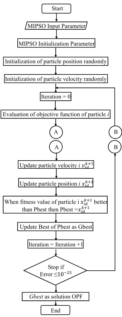
The optimal solution is obtained by comparing the value of the objective function for all combinations of power generation [16]. Operating
costs are dominated by the cost of fuel on the evocation is used as an objective function. As shown on the Flowchart of MIPSO Algorithm which is proposed in this study is indicated in the following:
Start
MIPSO Input Parameter
MIPSO Initialization Parameter
Initialization of particle position randomly
Initialization of particle velocity randomly
Iteration = 0
Evaluation of objective function of particle i
A B
A B
Update particle velocity i
Update particle position i %
When fitness value of particle i % better than Pbest then Pbest =%
Update Best of Pbest as Gbest
Iteration = Iteration +1
Stop if Error ≤103 W
Gbest as solution OPF
[image:4.612.313.517.155.685.2]End
ISSN: 1992-8645 www.jatit.org E-ISSN: 1817-3195
3. SIMULATION AND RESULT
In the simulation of the application of the MIPSO Algorithm method is performed in 2 system cases:
1. Case IEEE 30 Bus system, and
2. Case 150 kV Interconnection System SULSELBAR.
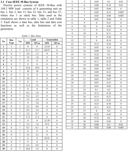
3.1 Case IEEE 30 Bus System
[image:5.612.88.525.191.709.2]Electric power systems of IEEE 30-Bus with 189.2 MW load consists of 6 generating unit on bus 1, bus 2, bus 13, bus 22, bus 23, and bus 27, where bus 1 as slack bus. Data used in the simulation are shown in table 1, table 2 and Table 3. Each shows a data bus, data line and data cost functions as well as the limitations of the generation.
Table 1. Bus Data
No Bus
Type Vm
Load Generation
MW MVar MW MVar
1 1 1 0 0 23.54 0
2 2 1 21,7 12,7 60.97 0
3 0 1 2,4 1,2 0 0
4 0 1 7,6 1,6 0 0
5 0 1 0 0 0 0
6 0 1 0 0 0 0
7 0 1 22,8 10,9 0 0
8 0 1 30 30 0 0
9 0 1 0 0 0 0
10 0 1 5,8 2 0 0
11 0 1 0 0 0 0
12 0 1 11,2 7,5 0 0
13 2 1 0 0 37 0
14 0 1 6,2 1,6 0 0
15 0 1 8,2 2,5 0 0
16 0 1 3,5 1,8 0 0
17 0 1 9 5,8 0 0
18 0 1 3,2 0,9 0 0
19 0 1 9,5 3,4 0 0
20 0 1 2,2 0,7 0 0
21 0 1 17,5 11,2 0 0
22 2 1 0 0 21.59 0
23 2 1 3,2 1,6 19.2 0
24 0 1 8,7 6,7 0 0
25 0 1 0 0 0 0
26 0 1 3,5 2,3 0 0
27 2 1 0 0 26.91 0
28 0 1 0 0 0 0
29 0 1 2,4 0,9 0 0
30 0 1 10,6 1,9 0 0
Table 2. Line Data
from bus
to bus
R X 1/2B
pu pu pu
1 2 0.02 0.06 0.015
1 3 0.05 0.19 0.01
2 4 0.06 0.17 0.01
3 4 0.01 0.04 0
2 5 0.05 0.2 0.01
2 6 0.06 0.18 0.01
4 6 0.01 0.04 0
5 7 0.05 0.12 0.005
6 7 0.03 0.08 0.005
6 8 0.01 0.04 0
6 9 0 0.21 0
6 10 0 0.56 0
9 11 0 0.21 0
9 10 0 0.11 0
4 12 0 0.26 0
12 13 0 0.14 0
12 14 0.12 0.26 0
12 15 0.07 0.13 0
12 16 0.09 0.2 0
14 15 0.22 0.2 0
16 17 0.08 0.19 0
15 18 0.11 0.22 0
18 19 0.06 0.13 0
19 20 0.03 0.07 0
10 20 0.09 0.21 0
10 17 0.03 0.08 0
10 21 0.03 0.07 0
10 22 0.07 0.15 0
21 22 0.01 0.02 0
15 23 0.1 0.2 0
22 24 0.12 0.18 0
23 24 0.13 0.27 0
24 25 0.19 0.33 0
25 26 0.25 0.38 0
25 27 0.11 0.21 0
28 27 0 0.4 0
27 29 0.22 0.42 0
27 30 0.32 0.6 0
29 30 0.24 0.45 0
8 28 0.06 0.2 0.01
ISSN: 1992-8645 www.jatit.org E-ISSN: 1817-3195 Tabel 3. The Generation cost function and Limits
Unit
Data Power Generation
Cost Function ($/Jam)
MW Limits
Min (MW)
Max (MW)
1 0 + 2 + 0.02 20 80
2 0 + 1.75 + 0.0175 20 80
3 0 + 1 + 0.0625 15 50
4 0 + 3.25 + 0.0083 10 55
5 0 + 3 + 0.025 10 30
6 0 + 3 + 0.025 12 40
The case of the IEEE 30-bus system used a parameter that is used to implement the MIPSO algorithm methods to complete generation optimization system of the IEEE 30-bus that is the value of the inertia weight (0.9-0.2) [11] total swarm = 50, maximum iterations = 1000, acceleration Coefficient = = 2.05, with total load of 189.2 MW.
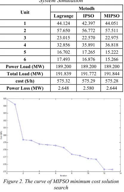
Table 4. Comparison of results of IEEE 30 Bus System Simulation
Unit Metodh
Lagrange IPSO MIPSO
1 44.124 42.397 44.051
2 57.650 56.772 57.511
3 23.015 22.570 22.975
4 32.856 35.891 36.818
5 16.702 17.265 15.222
6 17.493 16.876 15.266
Power Load (MW) 189.200 189.200 189.200
Total Load (MW) 191.839 191.772 191.844
cost ($/h) 575.32 575.29 575.28
[image:6.612.311.524.262.457.2]Power Loss (MW) 2.648 2.580 2.644
Figure 2. The curve of MIPSO minimum cost solution search
Simulated results on Table 4 showed that the most optimal solution obtained by MIPSO method with minimum fuel costs at 575.28 $/hour. The
search curve solution cost is reached at 13 number of iterations which is shown in Figure 2.
3. Case 150 kV Interconnection System SULSELBAR
In the case 150 kV Interconnection System SULSELBAR which consists of 7 thermal power generation and 3 water power generation, 28 bus and 34 channels. Table 5 shown a list of bus names and Type in the system.
Table 5. List of the name and bus type
No Bus
Type Bus Name No
Bus
Type Bus Name
1 2 Bakaru 15 0 Tallo Lama
2 0 Polmas 16 0 Sungguminasa
3 0 Majene 17 0 Tanjung Bunga
4 0 Mamuju 18 2 Tallasa
5 0 Pinrang 19 0 Maros
6 2 Parepare 20 1 Pagaya
7 0 Sidrap 21 0 Jeneponto
8 2 Balusu 22 0 Bulukumba
9 0 Barru 23 2 Sinjai
10 0 Pangkep 24 0 Bone
11 0 Bosowa 25 0 Soppeng
12 0 Kima 26 2 Sengkang
13 2 Tello 27 2 Makale
14 0 Panakukang 28 2 Palopo
Data of bus, line and cost function as well as the limitation of generation in the case of SULSELBAR 150 Kv Interconnection system is obtained from the data in field through PT. PLN (Persero) UPB region SULSELRABAR on March 11, 2015 At 19.30.
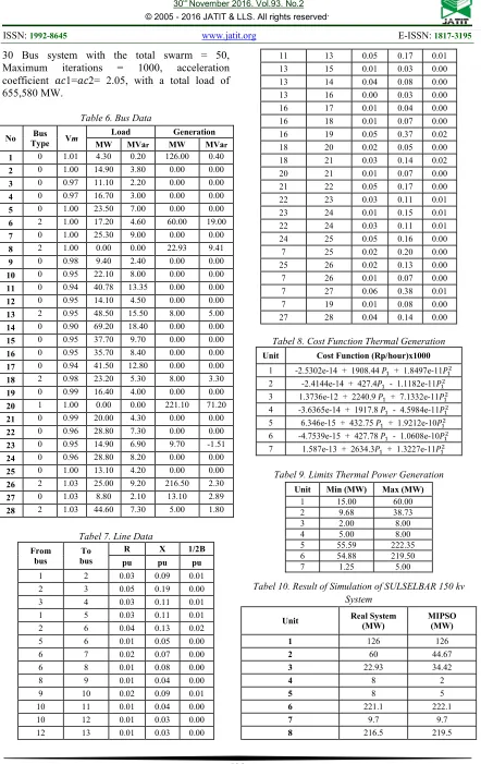
In table 6, The data bus in which the total load is at 655,580 MW, the data channel and the function of the cost of fuel thermal power generations is indicated in table 7 and table 8. For the data of the power generations (Bus 1 Bakaru - bus 23 Sinjai - bus 27 makale) in economic optimization simulation using MIPSO follow PT.PLN generation (Persero) is 126 MW for Bakaru, 9.7 MW for Sinjai and 13.1 MW for Makale. This is due to the operator of hydropower did not look at in terms of fuel costs, but the look of the pattern of water reserves in dams and reservoirs.
[image:6.612.92.300.372.692.2]ISSN: 1992-8645 www.jatit.org E-ISSN: 1817-3195 30 Bus system with the total swarm = 50,
[image:7.612.88.530.49.750.2]Maximum iterations = 1000, acceleration coefficient 1= 2= 2.05, with a total load of 655,580 MW.
Table 6. Bus Data
No Type Bus Vm Load Generation
MW MVar MW MVar
1 0 1.01 4.30 0.20 126.00 0.40
2 0 1.00 14.90 3.80 0.00 0.00
3 0 0.97 11.10 2.20 0.00 0.00
4 0 0.97 16.70 3.00 0.00 0.00
5 0 1.00 23.50 7.00 0.00 0.00
6 2 1.00 17.20 4.60 60.00 19.00
7 0 1.00 25.30 9.00 0.00 0.00
8 2 1.00 0.00 0.00 22.93 9.41
9 0 0.98 9.40 2.40 0.00 0.00
10 0 0.95 22.10 8.00 0.00 0.00
11 0 0.94 40.78 13.35 0.00 0.00
12 0 0.95 14.10 4.50 0.00 0.00
13 2 0.95 48.50 15.50 8.00 5.00
14 0 0.90 69.20 18.40 0.00 0.00
15 0 0.95 37.70 9.70 0.00 0.00
16 0 0.95 35.70 8.40 0.00 0.00
17 0 0.94 41.50 12.80 0.00 0.00
18 2 0.98 23.20 5.30 8.00 3.30
19 0 0.99 16.40 4.00 0.00 0.00
20 1 1.00 0.00 0.00 221.10 71.20
21 0 0.99 20.00 4.30 0.00 0.00
22 0 0.96 28.80 7.30 0.00 0.00
23 0 0.95 14.90 6.90 9.70 -1.51
24 0 0.96 28.80 8.20 0.00 0.00
25 0 1.00 13.10 4.20 0.00 0.00
26 2 1.03 25.00 9.20 216.50 2.30
27 0 1.03 8.80 2.10 13.10 2.89
28 2 1.03 44.60 7.30 5.00 1.80
Tabel 7. Line Data
From bus
To bus
R X 1/2B
pu pu pu
1 2 0.03 0.09 0.01
2 3 0.05 0.19 0.00
3 4 0.03 0.11 0.01
1 5 0.03 0.11 0.01
2 6 0.04 0.13 0.02
5 6 0.01 0.05 0.00
6 7 0.02 0.07 0.00
6 8 0.01 0.08 0.00
8 9 0.01 0.04 0.00
9 10 0.02 0.09 0.01
10 11 0.01 0.04 0.00
10 12 0.01 0.03 0.00
12 13 0.01 0.03 0.00
11 13 0.05 0.17 0.01
13 15 0.01 0.03 0.00
13 14 0.04 0.08 0.00
13 16 0.00 0.03 0.00
16 17 0.01 0.04 0.00
16 18 0.01 0.07 0.00
16 19 0.05 0.37 0.02
18 20 0.02 0.05 0.00
18 21 0.03 0.14 0.02
20 21 0.01 0.07 0.00
21 22 0.05 0.17 0.00
22 23 0.03 0.11 0.01
23 24 0.01 0.15 0.01
22 24 0.03 0.11 0.01
24 25 0.05 0.16 0.00
7 25 0.02 0.20 0.00
25 26 0.02 0.13 0.00
7 26 0.01 0.07 0.00
7 27 0.06 0.38 0.01
7 19 0.01 0.08 0.00
27 28 0.04 0.14 0.00
Tabel 8. Cost Function Thermal Generation
Unit Cost Function (Rp/hour)x1000
1 -2.5302e-14 + 1908.44 + 1.8497e-11
2 -2.4144e-14 + 427.4 - 1.1182e-11
3 1.3736e-12 + 2240.9 + 7.1332e-11
4 -3.6365e-14 + 1917.8 - 4.5984e-11
5 6.346e-15 + 432.75 + 1.9212e-10
6 -4.7539e-15 + 427.78 - 1.0608e-10
7 1.587e-13 + 2634.3 + 1.3227e-11
Tabel 9. Limits Thermal Power Generation
Unit Min (MW) Max (MW)
1 15.00 60.00
2 9.68 38.73
3 2.00 8.00
4 5.00 8.00
5 55.59 222.35
6 54.88 219.50
7 1.25 5.00
Tabel 10. Result of Simulation of SULSELBAR 150 kv System
Unit Real System (MW) MIPSO (MW)
1 126 126
2 60 44.67
3 22.93 34.42
4 8 2
5 8 5
6 221.1 222.1
7 9.7 9.7
ISSN: 1992-8645 www.jatit.org E-ISSN: 1817-3195
9 13.1 13.1
10 5 1.25
Power Load (MW) 655.580 655.580
Total Load (MW) 690.33 677.74
Cost (Rp/hour) x1000 376549 324842
Power Loss (MW) 27.408 28.308
Diference in cost
(Rp/hour) x1000 - 51.707
Figure 3. the curve of MIPSO search of minimum cost solution
The results of MIPSO simulations that are compared with real system data of PT. PLN (Persero) indicated in table 10. Economical optimization solutions that are visible by the method of MIPSO with the total cost per hour of Rp.324,842,000.- compared with real data sytem with total cost at Rp. 376,549,000.-per hour, so the costs that can be reduced by MIPSO method is at Rp.51,707,000.-. A search of the optimal solution of the economy reached at the 14th iteration as shown in Figure 3.
4. CONCLUSION
Based on the results of simulations using MIPSO method, the result simulated in IEEE 30 bus system as a form of validation showed minimum of 575.28 ($/hour) as compared to the Lagrange method at 575.32 ($/hour) and the IPSO at 575.29 ($/hour), and then MIPSO method is simulated in the SULSELBAR 150 Kv Interconnection system which compared to the real system operating costs amounting to Rp. 376,549,000,- per hour decreased to Rp. 324,843,000,- per hour, so there is a cost savings at about Rp. 51,706,000.- or around 13.73%.
REFRENCES:
[1] James Kennedy and Russel Eberhart, “Particle Swarm Optimization”, IEEE, 1995, pp1942-1948.
[2] Y.Shi, R.Eberhart. A Modified Particle Swarm Optmizer. Proc. IEEE Int. Conf. Evol. Comput. May 1998; pp 69-73.
[3] Kwang Y. Lee, and Jong-Bae Park, “Application of Particle Swarm Optimization to Economic Dispatch Problem: Advantages and Disadvantages”, IEEE Transactions on Power Sistems, 2006, 188-192.
[4] C. H. Chen, and S. N. Yeh, “Particle Swarm Optimization for Economic Power Dispatch with Valve-Point Effect”, IEEE PES Transmission and Distribution Conference and Exposition Latin America, Venezuela, 2006, pp 1-5.
[5] Habiabollahzadeh, H., Luo, G., Semlyen, A.: ‘Hydrothermal optimal power flow based on combined linear and nonlinear programming methodology’, IEEE Trans. Power Syst., 1989, 4, (2), pp. 530–537
[6] R.C. Eberhart, Y. Shi. ‘Comparing Inertia Weight and Constriction Factors in Particle Swarm Optimization’. Proceding of the 2000 Congress on Evolutionary Computation. 2000; Vol. 1, ,pp. 84-88.
[7] Niknam, T., Narimani, M.R., Aghaie, J., Azizipanah-Abarghooee.R. “Improved particle swarm optimisation for multi-objective optimal power flow considering the cost, loss, emission and voltage stability index” IET Gener. Transm. Distrib., 2012, Vol. 6, Iss. 6, pp. 515-527
[8] Nebro AJ, Durillo JJ, Nieto G, Coello CC, Luna F, Alba E. SMPSO: “a new PSO-based metaheuristic for multi-objective optimization”. In: IEEE Symposium on Computational Intelligence in Multicriteria Decision-Making 2009;1: 66-73.
[9] Maickel Tueguh, Adi Soeprijanto, Mauridhi Hery Purnomo, “Modified Improved Particle Swarm Optimization For Optimal Generator Scheduling”, Seminar Nasional Aplikasi Teknologi Informasi (SNATI), Yogkarta, 2009, pp 85-90.
ISSN: 1992-8645 www.jatit.org E-ISSN: 1817-3195 [12] M. Clerc. “The Swarm and The Queen:
Towards a Deterministic and Adaptive Particle Swarm Optimization”. Proc. 1999 Congress on Evolutionary Computation, Washington, DC Piscataway, NJ: IEEE Service Centre, 1999; pp. 1951-1957.
[13] Zhiyu You, Weirong Chen, Xiaoqiang Nan. Adaptive Weight Particle Swarm Optimization Algorithm With Constriction Factors. International Conference of Information Science and Management Engineering, 2010. [14] SailajaKumari, M., Maheswarapu, S.:
‘Enhanced genetic algorithm based computation technique for multi-objective optimal power flow solution’, Int. J. Electr. Power Energy Syst., 2010, 32, (6), pp. 736– 742.
[15] Shi Yao Lim, Mohammad Montakhab, and Hassan Nouri, “Economic Dispatch of Power System Using Particle Swarm Optimization with Constriction Factor”, International Journal of Innovations in Energy System and Power, Vol 4 No 2, October, 2009, pp 29-34. [16] Yusran, Ashari, M., and Soeprijanto,A.,