BIROn - Birkbeck Institutional Research Online
Wright, Stephen (2006) Tobin’s q and intangible assets. Working Paper.
Birkbeck, University of London, London, UK.
Downloaded from:
Usage Guidelines:
Please refer to usage guidelines at or alternatively
Tobin’s
q
and Intangible Assets
Stephen Wright,
Birkbeck College,
University of London
[email protected]
April 4, 2006
Abstract
1. Introduction
In a recent paper Laitner & Stolyarov (2003) assert that measured Tobin’s q has usually been well above 1, and use this as supporting evidence for their conclusion that there are significant quantities of unrecorded intangible assets. This key feature is referred to repeatedly in the paper to motivate their analysis.1
On closer examination this key piece of evidence turns out to be simply incor-rect. Laitner and Stolyarov’s q estimate is typically above unity solely because of number of clear errors in the way that the authors construct their data. They both overestimate the numerator and underestimate the denominator of q. The latter error is most significant: the primary factor being the omission of significant elements of tangible, rather than intangible assets - most notably land. When the calculation is carried out correcting for these errors the resulting q series turns out to be usually well below unity.
Even this corrected measure arguably has some major conceptual problems. Laitner & Stolyarov refer to the numerator of q as “stock market value”. Yet typically around a half to two thirds of the notional market value series in the numerator is an estimate of the value of unincorporated business for which there is virtually no true market value data. When calculated using market value data for the corporate sector alone, q is typically even further below unity.
In this short note I briefly describe the problems with Laitner & Stolyarov’sq
data, and illustrate the comparison between the original and corrected series with two charts. I also briefly discuss the puzzle of why q estimates might be so low. An Appendix provides a summary description of data construction and a table with corrected data.2
1To quote from their abstract; from their opening paragraph; and from Section IV (page
1258, referring to their Figure 1, which shows theirqestimate):
Tobin’s average q has usually been well above 1....The stock market value in the numerator of q reflects ownership of physical capital and knowledge, but the denominator measures just physical capital. Therefore q is usually above 1....Figure 1 suggests .. that the stock of applied knowledge (A) is 30-50 percent as large as the physical capital stock (K)...
2A full description of data construction is provided, for the benefit of referees, in Appendix
2. Comparing
q
Estimates
2.1. Replicating Laitner & Stolyarov
The data used for charts in this paper update Laitner & Stolyarov’s original q
estimates to include more recent data. In Appendix A, Table A1, I show that the correspondence between the original and recalculated series over their common data sample is extremely close.3 A key feature of the recalculated q series, as for
Laitner & Stolyarov’s original series, is that most observations are greater than unity. This feature is unsurprisingly particularly marked in recent years.
2.2. Correcting the numerator
The numerator of Laitner & Stolyarov’s measure ofqis intended to be an estimate of the market value of the entire business sector, made up of both corporate and unincorporated businesses. The authors calculate this value by residual from the net wealth of the personal sector, and the net liabilities of the government, overseas and the monetary authority, taken from the Flow of Funds tables. This apparently simple formula has the following drawbacks:
1. It includes the market value of holdings of equities of overseas corporations by US residents as well as the (empirically trivial) value of gold and SDRs;
2. It includes the value of net overseas direct investment by US corporations, and is therefore not directly comparable with the capital stock data;
3. It imputes all unidentifiedfinancial liabilities to the business sector.
The first two of these are clear errors; the third is at best a contentious as-sumption. An alternative estimate of the numerator that does not have these drawbacks can be constructed relatively straightforwardly (albeit more labori-ously) by adding up individual sectoral components using data from the Flow of Funds tables (for details see Appendix).
3Although there is an additional caveat that the formula for market value in terms of source
2.3. Correcting the denominator
The denominator ofqshould equal the replacement value of all the physical assets owned by the domestic business sector. The series used by Laitner & Stolyarov is given by the sum of the private nonresidentialfixed capital stock and nonfarm inventories. This measure too has very clear-cut drawbacks:
1. It contains some nonresidential fixed assets that should not be included, namely those belonging to households and non-profit making institutions.
2. It omits business residential capital (dominated by tenant-occupied housing owned by the noncorporate business sector)
3. It omits the value of land.
The first two defects can be easily rectified using published data.4 Land
presents somewhat more of a problem. The Fed do not publish data on land directly, but instead, for the non-farm, non-financial business sector, replace BEA series for structures with alternative estimates of real estate values: ie, the value of structures plus the land they sit on. Implicitfigures for the value of land can be derived as the difference between these two series.5 For these sectors I use
Fed data and thus deal with all three shortcomings simultaneously. For the other business sectors - farms and financial corporations - for which the Fed do not produce real estate data, I have attempted to mimic Fed methodology as closely as possible. However, since the available Fed data cover nearly 90% of total es-timated business tangible assets, the results are not sensitive to the inclusion of those missing elements for which they do not provide data.
4I again use data from the Federal Reserve Flow of Funds tables where available, but these
are derived from, and correspond closely to, the equivalent BEA series.
5The Fed used to publish these implied landfigures in their balance sheets but not longer do
2.4. The impact of the corrections
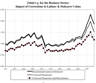
Tobin's q for the Business Sector:
Impact of Corrections to Laitner & Stolyarov's data
0.000 0.500 1.000 1.500 2.000 2.500
1952 1957 1962 1967 1972 1977 1982 1987 1992 1997
Recalculated Laitner & Stolyarov Corrected Numerator
[image:6.595.143.468.157.440.2]Corrected Numerator and Denominator
Figure 1
Figure 1 shows the impact of the two sets of corrections alongside the recal-culated estimate using Laitner & Stolyarov’s approach. The second line shows the impact of amending the formula for the numerator, which has a fairly modest impact except in recent years. The third line shows the much more significant impact of correctly defining the denominator (the inclusion of residential capital and land have a more or less equal impact). The net result of all the corrections is that in 2000, close to the peak of the market, Laitner & Stolyarov’sqestimate was around 60% higher than the corrected measure using identified market value.The chart also clearly shows that the corrected q series, far from being predominantly above unity, is predominantly below.6
6In Appendix B I discuss an alternative treatment of land and residential capital which
2.5. Sectoral q data
Sectoral q Estimates
0.0 0.2 0.4 0.6 0.8 1.0 1.2 1.4 1.6 1.8
1952 1957 1962 1967 1972 1977 1982 1987 1992 1997 2002
Nonfarm Nonfinancial Corporations Noncorporate + Farms All Corporations
Figure 2
The corrected q series shown in Figure 1 builds up both numerator and de-nominator from their sectoral components. An advantage of this approach is that it is possible to examine the implied sectoralq estimates that underlie the aggre-gate figures for the business sector. These, shown in Figure 2, strongly reinforce the picture ofq as being predominantly well below unity for those sectors where market valuations are available.
Typically around a half to two thirds of the notional market value of the busi-ness sector as a whole is made up of the value of unincorporated busibusi-ness. This series is calculated from net liabilities (of which only a very small fraction are marketed securities) plus the imputed value of equity in unincorporated business. This latter figure (itself the dominant element in total value) is constructed by simply cumulating net investment flows. Unsurprisingly, therefore, the resulting
In contrast the market value of the corporate sector is dominated by stock market valuations,7 and as such corresponds much more closely to the measure
of q that Laitner & Stolyarov analyse in their model. Figure 2 shows that this series is distinctly more volatile than the aggregate series in Figure 1.8 It is also
of course distinctly lower: indeed it only rose above unity for the first time at the height of the boom in the 1990s. Thus there is strong evidence that, where market valuations exist, the resulting measure of q is systematically well below, rather than above unity.
3. Conclusions
This note has focussed on the empirical basis for the recent claim made by Laitner & Stolyarov (2003) that Tobin’s q is typically above unity, which they use as supporting evidence for their conclusion that intangible assets are quantitatively significant.9 It turns out that, once correctly calculated using available data,
Tobin’s q has instead typically been wellbelow unity. This conclusion is strongly reinforced ifq is measured only for sectors where market valuations actually exist. The fact that, once correctly calculated, measured q is systematically less than unity is a puzzle that deserves attention. It does not, of course, mean that intangible assets do not exist; it just means that their existence or their magnitude cannot be inferred straightforwardly from the properties ofq. It also means that if they do exist in significant quantities either statisticians or markets must be getting something systematically wrong. Indeed this conclusion is inescapable, whatever the value of intangible assets, since even on the basis of tangible assets alone measuredq is systematically below unity.
Two possible problems with the statisticians’ approach might be that the
7These include Fed estimates of imputed values of unquoted securities.
8The chart also shows that movements inqfor the corporate sector as a whole are dominated
by those ofqfor the non-farm non-financial corporate sector, which can be derived entirely from Fed data. The implied q estimate for financial corporations, which relies in part on my own estimates (albeit following Fed methodology wherever possible, see Appendix B) is distinctly more volatile but is also typically below unity.
BEA’s capital stock data may be based on overstated assumed capital lives, or that investment deflators may be incorrectly calculated (as proposed, for example by Gordon, 1990). The alternative explanation, that markets may have systemat-ically under-valued corporate assets over a long period, is probably more worrying for those who believe that market valuations are at least on average rational; but should not be entirely ruled out purely on these grounds. The puzzle of whyq is usually less than unity certainly merits further investigation.
Afinal, and important, if rather uncomfortable conclusion for applied macro-economists is that Laitner & Stolyarov’s errors provide something of a cautionary tale. Data construction, while undeniably tedious, is not something that can be hurried or glossed over. The simple and quick calculations they carried out pro-vided interesting results that appeared to provide significant support for their modelling approach. But these results were incorrect, and, with due care, avoid-ably so. Since their results were published in a major journal, the key feature they mistakenly ascribed toq is likely to acquire the status of a “stylised fact”, if not corrected. That is the purpose of this short note. 10
10My critique of Laitner & Stolaryov’s errors and omissions in data construction does not of
APPENDIX
A. Summary of Data Construction
Table A1 provides a summary of the corrections to data in Laitner & Stolyarov (hereafter LS). For full (and very tedious) details the interested reader is referred to Appendix B. A spreadsheet containing all series and their underlying components, the sheets of which correspond to the panels of Appendix B Table A2 is also available on request. All source references below are to Flow of Funds (Z1) tables (Federal Reserve, 2004), except those to TA, which refer to the BEA tangible assets tables, and NIPA, which refer to National Income and Product Accounts tables.
Column 1, "Business Fixed Capital and Inventories": This series is taken directly from LS Table A1, and is as defined therein as TA 4.1 R1 + NIPA 5.75 R1. LS refer to this series as “business fixed capital and inventories” but it is more precisely defined as non-residentialfixed capital and inventories.
Column 2, "Market Value of Businesses": This series is also taken di-rectly from LS Table A1, but the definition given therein contains a significant number of errors and if applied to more recent data results in a series which is radically different. However, the authors have confirmed in email correspondence that the actual data were in fact defined by residual from the net worth of the household sector and non-profit making institutions, less the net liabilities of the government, monetary authorities and overseas. The corrected formula is: L100 R1 -L100 R24 +L105 R1+L105 R17 + L106 R1- L106 R13+ L107 R1 - L107 R23+L108 R1 + L1O8 R15
Column 3 gives Laitner & Stolyarov’s reported q series (ie, Column 1/Col-umn2) from their Table A1, while Column 4 gives the recalculated series on Laitner & Stolyarov’s definition, but using the corrected formula for market value.
Column 5, Business Tangible Assets: This series is built up from two
same ratio as for noncorporate business.11
Column 6, Reproducible Capital: This series is derived by replacing fi g-ures for real estate (ie structg-ures plus land) with those for structg-ures alone. As such it uses only published data. Nonfarm, nonfinancial business structures data are taken from the flow of funds tables but are consistent with BEA data. The precise definition is Column 4 -(B102 R3 + B103 R3 + financial corporations’ real estate + farm real estate) +(B102 R 32+ B102 R33+ B103 L32+B103 R33 +TA 4.1 R27 + TA4.1 R6 + TA 5.1 L18). Financial corporations’ and farm real estate are defined as in Appendix B Table A2 Panels M and N. In Panel G of the same table I also show that a virtually identical series can be built up directly from BEA tangible assets data.
Column 7, Market Value of US Business: In contrast to LS, who
con-struct business market value by residual, I build up this series from its individual components, all of which can be derived from the flow of funds tables. For each sector market value is defined as the sum of net identified liabilities plus the market value of equities. LettingM = market value, Column 6 can be defined as:
MDomestic Business =MNonfinancial+MFinancial−Net ODI
whereMNonfinancial =Nonfinancial net liabilities (L101 R16-L101 R1)+ equities (L5
R23 + L102 R41); MFinancial =Financial corporations’ net liabilities12 (L5 R33-L5
R20+ L100 R1 -L100 R24 +L105 R1+L105 R17 + L106 R1- L106 R13+ L107 R1 - L107 R23+L108 R1 + L1O8 R15-L101 R16+L101 R1) + equities ( L213 R4); and Net ODI = net overseas direct investment (L230 R1-L230 R16). In Appendix B, Table A2 Panel D, I show that Column 2 (corrected definition)= Column 6 plus unidentified net liabilities (L5 R33-L5 R20-L5 R21-L5 R22-L5 R23) plus overseas corporate equities (L213 R3) + all sectors’ gold and SDRs (L5 R21), as described in Section 2.2.
Column 8 gives the corrected series for Tobin’s q (as shown in Figure 1), defined by Column 6 / Column 4
11I also discuss an alternative method of imputation of real estate values derived from mortgage
data, but I show that this has minimal impact on the aggregatefigure.
12This series is measured, for convenience, by residual from total identified stocks and the
References
[1] Federal Reserve (2000) Guide to the Flow of Funds Accounts, Board of Gov-ernors of the Federal Reserve System, Washington DC
[2] Federal Reserve (2004) Flow of Funds for the United States January 2004, Board of Governors of the Federal Reserve System, Washington DC
[3] Gordon, R J (1990) “The measurement of durable goods prices” National Bu-reau of Economic Research Monograph series Chicago and London: University of Chicago Press.
[4] Laitner, J and Stolyarov, D (2003), “Technological Change and the Stock Market”,American Economic Review, vol. 93, no. 4 1240-67
NOTE TO REFEREES
Appendices B and C are provided solely for the benefit of referees;
they could also in principle be made generally available in electronic form for any readers interested in such a level of detail, together with the associated dataset.
B. Full Details of Data Construction
Table A2 sets out the sources and data construction methods, which allows a direct comparison of the q estimates used in this paper with those in Laitner & Stolyarov (2003) (hereafter LS). The panels of Table A2 correspond to equivalent sections of a spreadsheet that is available on request. All source references therein are to Z1 (flow of funds) tables (Federal Reserve, 2004), except those to TA, which refer to the BEA tangible assets tables, and NIPA, which refer to National Income and Product Accounts tables.
B.1. Market Value
B.1.1. Replicating Laitner & Stolyarov
Panel A of Table A2 reproduces verbatim the formula for market value using the Flow of Funds table references as given in LS (P1261, footnote to Table A2). However, this formula results in a series which is radically different from their own reported series for market value (in Appendix A, col. 2), with the series con-structed using their reported formula exceeding their reported series by anything up to 50%.
B.1.2. Market Value from Identified Components
Panel C provides definitions underlying my alternative market value series that corrects the problems with the LS approach as set out in Section 2.2. It builds up the series by adding up identified components of market value usingflow of funds data on equities, assets and liabilities.13 These sum to a series which measures the identified value of US-owned business. To ensure complete comparability with tangible assets data, the data are then adjusted to provide the market value of domestic US business (ie, including the value of foreign companies’ operations in the US, but excluding the value of US companies’ operations abroad). Although this last adjustment is required in logic, it turns out to make (surprisingly) little difference to market value estimates.
Panel D shows how this approach can be reconciled with that of Laitner & Stolyarov. Their series does not correct for net ODI, and includes both US hold-ings of overseas equities and the very small category of other assets (gold and SDRs) not included in liabilities data. Their estimate also includes unidentified liabilities: the gap between total recorded assets and the sum of recorded liabilities and all assets not included in liabilities. This unidentified element in debt may indeed reflect unrecorded liabilities of US business, and thus it is of interest to see its impact; but anyone using this approach should be aware of its inclusion. The table shows that on average inclusion of unidentified debt slightly lowers measured
q(since for most of the sample unidentified debt was negative); however, this ele-ment switched sign quite dramatically in the 1990s, and by end-2002, unidentified debt was equivalent to 14% of identified business market value.
B.2. Reproducible Capital at Replacement Cost
Panel F of Table A2 reproduces the formula for businessfixed capital plus inven-tories used in LS: the resulting series is virtually identical.
Panel G provides an alternative formula based on BEA data. There are two key modifications. First, that part of nonresidential fixed capital belonging to the personal sector and non-profit making institutions is excluded, for consistency with the derivation of market value data. Second, a series is constructed for the residential capital stock of the business sector. Following the same methodology
13Thefinancial sector’s recorded assets and liabilities are measured, for convenience, by
as outlined by the Federal Reserve in constructing their tangible assets series (Federal Reserve, 2000, p299) for the nonfarm, noncorporate business sector, this subtracts the residential capital stock of non-profit making institutions, and of owner-occupied housing, from the private sector total (unlike the Fed approach tenant-occupied farm housing is retained since the definition here includes all farms). Total private inventories are then added to thefigure for fixed capital.
The resulting series for total business reproducible capital is systematically larger than the series used by LS, differing by a factor of around 20% in the early part of the sample, with the difference falling steadily to around 10% by the end of the sample. It is extremely close to the equivalentfigure derived on a Z1-equivalent basis, as described in the next section, never differing by more than around 1%.
B.3. Tangible Assets Including Land
Panel H of Table A2 summarises the construction of a series for business tangible assets including land. The series is built up from two elements (for the non-farm, non-financial corporate and non-corporate sectors) that can be taken direct from theflow of funds tables, plus equivalent series forfinancial corporations and farms, the construction of which (involving some guesswork) is summarised in Panels M and N.
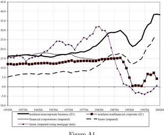
Figure A1 shows that the implied land series for the two sectors for which the Fed produces tangible assets data both show a distinct discontinuity after 1989, following a change in Fed methodology.14 The implied share of land for
nonfinancial corporates falls virtually to zero in the mid-1990s, but then recovers somewhat. The implied share of land for non-corporates shows a similar fall, but then recovers distinctly more strongly, to a much higher level (reflecting the much more significant proportion of residential capital for the non-corporate sector).
14See Wright (2004) for a discussion and a proposed alternative treatment that deals with
Implied and Imputed Shares of Land in Tangible Assets
-10.0 -5.0 0.0 5.0 10.0 15.0 20.0 25.0 30.0 35.0 40.0 45.0
195204 195704 196204 196704 197204 197704 198204 198704 199204 199704 200204 nonfarm noncorporate business (Z1) nonfarm nonfinancial corporate (Z1)
[image:16.595.145.467.157.422.2]financial corporations (imputed) farms (imputed) farms (imputed using mortgage data)
Figure A1
Panel M details the (fairly straightforward) construction of estimates of tan-gible assets for financial corporations. Data for structures and equipment and software come straight from the BEA nonresidential tangible assets series (Table 4.1). Both inventories and residential capital are set to zero, since these are already fully allocated to nonfinancial corporations in the flow of funds tables. Real estate figures are estimated by scaling BEA structures data using the ratio of real estate to structures for nonfinancial corporations. As Figure??shows, the resulting imputed share of land in tangible asesets is very similar to that for
non-financial corporations (the somewhat higher figure in earlier years reflecting the lesser importance of equipment and software of financial corporations compared to non-financials).
the basis of BEA structures figures on the same basis. Figure ?? shows that the resultingfigure for land appears distinctly conservative, since it is well below the share of land for non-farm non-corporates, despite the clearly land-intensive nature of farming.
As an alternative method of calculation, to provide at least a basis for com-parison, farm real estate values can inferred on the basis of farm and household sector mortgages (lines 5 and 2 of Z1 Table L217, respectively), by working on the assumption that collateral ratios applied by lending institutions are the same, using the ratio of home mortgages to household real estate (Table L100, line 4). Land values are then inferred as the difference between the resulting real estate values and BEA data on farm structures. Figure ?? shows that this results in distinctly higher implied land values in the early part of the sample, but that the implied share of land then falls steadily, such that, by the end of the sample, it is slightly negative - which would imply that the BEA’s estimate of the replacement value of farm structures is greater than their market value including the land they sit upon.15 However, Figure ??shows that even this very extreme, and distinctly
pessimistic implication for farms has very limited implications for the resultingq
estimate for the non-corporate plus farm sector in aggregate.
B.4. An alternative measure of q
As noted in Section 2, it is possible to derive an alternative measure of q with a different treatment of land and both residential and nonresidential structures, if real estate valuations used by the Fed can be assumed to be directly comparable to stock market valuations. If the additional assumption is made that q is the same for all elements of capital, this implies the alternative definition:
q∗ = total market value - value of real estate
total reproducible capital - structures (B.1)
with an associated estimate of land:
land=value of real estate −q. structures (B.2)
The rationale underlying this alternative estimate is that both elements of the numerator in (B.1) are mutually consistent market valuations. Figure A2 shows the resulting time series forq∗.
15This somewhat surprising result does not appear to be due to a fall in the importance of
Impact of Corrections to Laitner & Stolyarov's data: An Alternative Estimate of q
-0.500 0.000 0.500 1.000 1.500 2.000 2.500 3.000
1952 1957 1962 1967 1972 1977 1982 1987 1992 1997
[image:18.595.145.463.136.422.2]Recalculated Laitner & Stolyarov Alternative estimate (q*) on corrected data
Figure A2
Figure A2 shows that the resulting series is radically more volatile, and in-cludes some extremely low observations (one is negative). The explanation is quite straightforward: the adjusted definition subtracts from both numerator and denominator the largest single component of corporate capital. As the ratio of two generally small numbers, each of which is the difference between two large numbers, the resulting series is extremely volatile.
C. Method of Moments Estimates of the Share of
Intangi-bles
While the authors’ method of moments estimation procedure estimates six pa-rameters simultaneously, applying cross-equation restrictions across the six equa-tions of their model, there is one key empirical relaequa-tionship that determinesθ,the steady-state share of the intangible capital stock in total capital. In their Cobb-Douglas framework, and working in terms of steady state ratios for simplicity, this is given by
θ = α
α+β ≡ A
A+K∗ (C.1)
where A is intangible capital, K∗ is the measured capital stock, and α and β
are their respective exponents in the production function. Substituting from the authors’ equation (19) into (22) implies that in steady state
IK
M = (1−θ)
£
gMi+δ¤ (C.2)
where (using their definitions),IKis gross recorded investment,M is market value,
gMi= Mt−Mit−1 i
Mt−1 is a “revolution-adjusted” measure of growth of market value, that
strips out the one-off effect of the single technological innovation;16 and δ is the
true depreciation factor. The authors’ estimate of θ is greater than zero because recorded investment is “too low” in relation to market value to be consistent with growth rates and depreciation.
The authors do not include the measured capital stock K∗ in their
empiri-cal model directly, but do include it indirectly, since they have an equation for recorded depreciation, given in their model by D = δK∗ where δ > δ is the
av-erage depreciation rate. (In their framework this is higher than true depreciation due to the impact of periodic technological innovations). Using this definition, the evolution of measured tangible capital (excluding land) in steady state implies
IK
K∗ =gK∗+δ. (C.3)
Combining (C.2) and (C.3) implies
1−θ = 1 qLS
µ
gK∗+δ gMi+δ
(C.4)
The second ratio on the right-hand side of (C.4) is very close to unity;17 indeed
it should be precisely unity ifM andK∗ are not to drift apart indefinitely. Thus,
on a single equation basis, the fact that their estimate of θ greater than zero relates directly to qLS being above unity on average (in practice cross-equation
restrictions complicate matters somewhat).
Give the shortcomings of the authors’ q data as described in Section 2, one obvious explanation of their estimate ofθbeing greater than zero is that it reflects, wholly or in part, omitted elements of tangible, rather than intangible assets, most obviously the exclusion of land. Using Laitner & Stolyarov’s own results, it is possible to derive a simple test of the hypothesis that land is the sole explanation.
With three forms of capital, the steady state value of θ will be given by
θ = A+L
A+L+K∗ (C.5)
where A is intangible capital and L is land. Deriving implicit land values as described in Section 2.3, we can derive an estimate of L/(L+K∗), the steady-state share of land in total tangible assets, which has a sample average of 14%. The hypothesis thatA = 0thus implies θ =.14, hence, using (C.1) we haveH0 :α = ¡0.14
0.86 ¢
β ⇒ α−.167β = 0, a simple linear restriction. Laitner & Stolyarove have kindly provided an amended set of empirical results (and the Fortran program that generates these) in which investment and depreciation figures are adjusted from the original series to include investment in residential capital as described above, but landfigures are excluded. Using their estimated parameter covariance matrix, the standard error of the linear combination αb −.167β,b results in a t-statistic of just 1.84 for the test of the implicit null thatA= 0.This seems a very slender statistical thread on which to hang an assertion that there is a significant quantity of unmeasured intangible capital, especially given the other problems with both market value and land data for the business sector discussed above.18
17My best guess at a point estimate, using the authors’ empirical estimates and appropriately
adjusted growth rates, is 1.004. In Laitner & Stolyarov’s framework M typically grows more rapidly thanK∗,and depreciates more slowly; but is lowered periodically by structural shocks when “revolutions” happen; the higher depreciation rate for K∗ reflects the average effect of these shocks, since the level ofK∗ is never hit by these negative shocks.
18Especially the weaknesses of the land data, and the dominant role of the noncorporate sector
Table A2 Detailed Data Definitions for Comparison with Laitner & Stolyarov (2003)
A.Market Value as defined in Laitner & Stolyarov
less Less less plus plus Plus minus Minus plus minus Equals
Source: L100, R1 L100, R25 L106, R15 L105, R18 L105,R7 L105,R1 0 L108, R10 L106, R14 L108, R15
L107, R1 L107, R23 Househol ds and non -profit Househol ds and non -profit Fed governm ent State & local governm ent State & local governm ent State & local governm ent Monetary Authority (excl FRB) Fed governm ent Monetary Authority (excl FRB) Rest of World Rest of World Total Business, L&S definition Financial Assets total liabilities Treasury currency (liabilitie s) Credit market liabilities US gov't securities (assets) municipa l securities (assets) US gov't securities (assets) SDRs (liabs) Total liabilities total financial assets total liabilities Implied market value
B. Alternative calculation of Market Value as in Laitner & Stolyarov
Less plus less plus Less plus Minus Plus plus Equals
L100, R1 L100, R25
L105, R1 L105, R17
L106, R1 L106, R13
L107, R1 L107, R23
L108, R1 L108, R15
Household s and non -profit Househ olds and non -profit State & local governm ent State & local governm ent Fed governm ent Fed governm ent Rest of World Rest of World Monetary Authority (excl FRB) Monetary Authority (excl FRB) Total business, L&S definition
C. Market Value from Identified Components
minus plus plus plus equals Plus minus plus Equals minus Plus equals
L101,R1 L101,R16 L5,R23 L102, R41 L213,R4
Panels B, C and D
Panels B, C
and D L230, R1 L230, R16
non-financial business non-financial business non-corporate business non-financial corporations non-financial business financial corporations financial corporations financial corporations Total business total business total business total business total financial assets total liabilities household equity in noncorp business value of equities (including farm equities) market value of US nonfinancial business value of equities total financial assets total liabilities Identified market value of US business
Stock of US direct investment abroad Stock of foreign direct investment in US Identified Market Value of Domestic Business Capital
D: Reconciliation of Identified Market Value with Laitner & Stolyarov Market Value
Minus minus Equals plus plus Plus equals
L5 row 33 L5, R20 L5, R21 to R23 Panel C L213, R3 L5, R21 Panel B
all sectors all sectors rest of world all sectors
total business
Assets not
F. Capital from BEA nonresidential data (as in Laitner & Stolyarov)
Plus equals Cf
TA 4.1, R1 NIPA 5.75A, R1 Laitner & Stolyarov
Private Private private
non-residential fixed assets Inventories non-residential fixed capital and
inventories
"business fixed capital and inventories"
G. Alternative BEA capital measure data excluding non-business non-residential capital but including residential capital
Less less equals Plus Less Less equals Plus equals
TA 4.1, r1
TA 4.1, R46
TA 4.1, R49 TA 5.1,
R2
TA 5.1, R6
TA 5.1, R 14 NIPA
5.75A&B L1 private non-profit
institution s
persons business Private non-profit
institution s
owner-occupied
business Private business
non-residentia l fixed assets non-residential fixed assets non-residential fixed assets non-residentia l fixed assets residentia l fixed assets residential fixed assets residential fixed assets
total fixed assets Inventories (end-year)
H. Tangible Assets from flow of funds, BEA data and proxies for land
Plus Equals Plus plus equals
b102, r2 b103, r2 Panel M Panel N
nonfarm non-financial corporate
nonfarm non-corporate
nonfarm non-financial business
financial corporations farms business
tangible assets (inc land) tangible assets (inc land)
tangible assets (inc land)
tangible assets (inc land) tangible assets (inc land) Tangible assets (inc land)
M: Actual and imputed tangible assets of financial corporations
equals Of which: Plus Plus Plus
TA 4.1 L 27 TA 4.1 L 26
Tangible assets
real estate (using ratio to structures from nonfinancials), o/w
Structures, of which
Non-residential structures, direct from BEA
Residential structures (set to zero, since Z1 imputes all to
nonfinancials)
Land (residual)
nonresidential equipment and software, direct from BEA
N: Actual and imputed tangible assets of farms (corporate and noncorporate) using BEA tangible assets
Equals of which: plus plus plus plus
Imputed TA 4.1
L6
TA 5.1, L18
TA 4.1 L5 imputed NIPA
5.75A L2
Tangible assets
real estate (using ratio to structures from nonfarm noncorporates)
Structure s, of which
Non-residentia l structures , direct from BEA
residentia l
structures (only tenant-occupied)
Land (residual)
nonresidential equipment and software, direct from BEA
residential equipment and software (using ratio for nonfarm noncorporates)