7293
NEGATED ITEMSETS OBTAINING METHODS FROM
TREE-STRUCTURED STREAM DATA
JURYON PAIK
Pyeongtaek University, Department of Digital Information and Statistics, Gyeonggi-do 17869, South Korea E-mail: [email protected]
ABSTRACT
With the rapid development of Internet of Things technologies, millions of physical objects communicate each other and produce huge volumes of data. The IoT revolution comes great opportunities and changes the world completely, but also increases the difficulty of data usage. Along with fusing the cutting-edge technologies, the challenge is the development of software and analytical systems that turn the deluge of massive data produced by different applications over sensor networks and internets into valuable and useful information. One of the popular method is to discover interesting relations between data. However, finding hidden information from xml-based data is not easy task to do. To make matter worse, it is much more difficult if the discovering relation is for between non-exiting parts of data. In this paper, we are trying to figure out how efficiently find out the important non-existing data parts from xml-based data and provide some definitions with adjusted formulas tailored to our target data along with an framed algorithm.
Keywords: Negated Tree Items, Negative Association Rules, XML Neraged Items, Tree Data, Association
Rules
1. INTRODUCTION
Enabled by communications and sensor technologies, the Sensor Web in the big data era shares, finds, and accesses sensors and their data across different applications over a sensor networks and the web [1,2]. Sensor Web technologies provide real-time or almost real-time data and reliable monitoring it to support agile decision making and alter fundamentally the way we live. With increasingly integrating sensors and wireless communications, the sensor web is possible to detect, identify, and cover a diverse range of stream data types, from simple raw data set to complex structure data set. It is required to handle efficiently and exchange desirably the large heterogeneous stream datasets. That is using XML-based data format, which is the de facto standard for exchanging and modeling data from a wide variety of sources over the web. Also, it is used as a serialization format in a semantic web context.
Fused with disruptive technologies such as integrating sensors and wireless communication, managing big data and data analytics, and building the sensor web, the cutting-edge environment inevitably produces tremendous volumes of stream data. Researchers and venders are gaining the capability to gather sufficient data. But, to achieve
actual improvements or innovations in development outcomes, it has to be preceded to turn the deluge of data into useful and valuable information.
One of the well-known methods is to discover interesting relations between data, called association rules mining. In recent years, there has been a significant research focused on finding interesting non-existing or infrequent parts of data leading to the discovery of negative association rules [3]. However, the discovery of non-existing data parts is far more difficult than their counterparts, that is, frequent data parts. Besides, it is the most difficult task if the data type is complex structure like xml. Analyzing continuously arriving xml data is intricate and complicated process, and many of the problems it presents have yet to be adequately solved. It is still in an immature stage and not fully developed to address the problem of finding negative association rules from xml-based stream data.
The main contribution of this paper is to describe what is the negative association rule, what is required to discover non-existing data parts, and what is the efficient way to generate negative association rules for xml-based dataset.
2. RELATED WORK
7294 rapidly increasing sensor network deployments and the ability to generate large volumes of data in current Internet of Things (IoT) infrastructure, the researchers have burst into finding association rules from the stream data. Among the early studies on stream data from sensors, Loo et al. [4] proposed a framework for discovering association rules from sensor networks. In their approach, sensors’ values are considered mainly to generate the association rules and the time is divided into intervals. With interval list based lossy counting, transaction in Loo
et al.’s data model, the size of data structure is significantly reduced.
With growing data volumes and increased data complexity, the importance of negative association rules is even bigger than that of positive association rules. However, there are very few research works conducted on mining negative association rules over streaming data. Most of the published articles are confined to static database environment [5-8]. The reason the researches for negative association rules are much less than that of positive ones is that there are fundamental differences between them, as described by Wu et al. [9]. While positive association rules are generated with frequently occurred itemsets, negative association rules are generated with infrequently occurred or absent itemsets. That means we must search a gigantic number of negative association rules even though the database is small. If the database becomes larger, it would be more difficult. Particularly, it is a challenge to identify which rules are beneficial or useful to applications from the enormous and rigorous size of streaming data.
The algorithm MPNAR-SW proposed by Ouyang [10] mines both positive and negative association rules from data stream. It applies so called transaction-sensitive sliding windows. In the algorithm, a bit-sequence Bit(X) is constructed for each item X in a current sliding window. If an item X is in the ith transaction of the current window, the
ith bit of Bit(X) is set to be 1; otherwise, it is 0. In this way, each item on the incoming transactions is transferred into its bit-sequence representation. The suggested MPNAR-SW consists of four phases, and the bit-sequenced stream data through the phases 1 and 2 is used to generate frequent, infrequent itemsets at the 3rd phase. And at the 4th phase, positive and negative association rules are produced from the outputs of the previous phase. The author states it is the first research work conducted on finding negative association rules over data streams. However, the algorithm is not cost-effective because
it has the same approach with the time-consuming Apriori algorithm for generating positive rules.
Corpinar and Gündem [11] suggest a rule mining system that provides solution to positive and negative association rules computation. However, their type of data stream is different to that of other approaches. The data is XML data stream. To achieve the goal, they first adapt the original FP-Growth method to support stream data mining and negative rules. To decrease the search space for negative association rules, they devised new pruning thresholds along with adding correlation coefficient parameter into their methodology to separate the frequent sets for positive and negative rules.
The recently published paper [12] presents several new definitions and scheme related to association rule mining over xml data streams in wireless sensor networks. The authors’ proposed scheme is the first approach to mining association rules from xml stream data in the sense that it generates frequent tree items without any redundancy. The overall methodology can be applied to any individual block, as well as the whole stream.
In this paper, we focus on the problem of extracting informative tree-structured itemsets for negative association rules from stream xml data. We consider pruning techniques because negative association rules are built from a huge number of infrequent and negated tree items. We mainly discuss two major methods, interestingness vs. correlation coefficient, for the pruning phase. Then, we show different results obtained by the two measuring factors with simple examples based on a frame algorithm and compare them.
3. BACKGROUND CONCEPTS
3.1 Negative Association Rules
7295 buy bread usually purchase milk. 3) ¬bread ¬milk, the customers who do not buy bread usually do not purchase milk, either. The symbol ¬ means absent, non-existing, or formally negated. This paper considers the form X⇒ ¬Y for convenience.
To select interesting rules from the set of all possible rules, constraints on various measures are used. The best-known constraints are minimum thresholds on support and confidence [14]. When I
= {I1, I2 … In} is a set of items from a transaction database D, and XY (XI∧YI∧XY = ) is a positive association rule, a support of X with respect to D is defined as a proportion of transactions that contains all items in X, which is the function
sup(X) = |X|/|D|. Support is an indication of how frequently the itemset appears in the dataset. Hence,
sup(X ⇒Y) means the support of an union of the items in X and Y, sup(X ⇒Y) = |X Y |/|D|. The confidence is an indication of how often a rule, X
Y, has been found to be true, that is the proportion of the transactions that contains X which also contains
Y, written as the function conf(X⇒Y) = sup(X⇒Y)/
[image:3.612.115.277.385.455.2]sup(X) = |XY |/|X|.
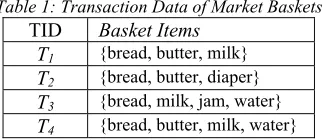
Table 1: Transaction Data of Market Baskets
TID Basket Items
T1 {bread, butter, milk} T2 {bread, butter, diaper} T3 {bread, milk, jam, water} T4 {bread, butter, milk, water}
Table 1 shows an extremely small example of a market basket domain. The set of items I = {bread, butter, diaper, jam, milk, water} and the table is a transaction database D. Each transaction Ti
(1 ≤ i ≤ 4) contains several items in I. Suppose there is an example rule bread milk meaning that if bread is bought, customers also buy milk. The support value of this rule, sup(X⇒Y), is the support of itemset {bread, milk}, which has a support of 3/4 = 0.75 since it occurs in 75% of all transactions (3 out of 4 transactions). The confidence value of the rule is determined by 3/4 = 0.75 in the database. It clearly means that for 75% of the transactions containing bread the rule is correct (75% of the times a customer buys bread, milk is purchased as well).
The second example rule is {bread, butter} ⇒milk. It has a support of 2/4 = 0.5 and a confidence of 2=3 ≈ 0:66, which states that customers who buy bread and butter also buy milk in more than 66% of the cases and this rule holds for 50% of the entire transactions. Adding the item ‘butter’ reduces the support value from 0.75 to 0.5 because it makes the
rule more restrictive. With the useful relationships among the underlying data, market managers will put bread, milk, and butter together, and this may increase their profits because the relationships identify new opportunities for cross-selling their products.
Presented by the simple examples, both measures count how many times itemsets appear in a dataset. Because negative association rules encapsulate the relationship between the occurrences of one set of items with the absence of the other set of items, the support and confidence of the rule X⇒ ¬Y must count non-existing items in transactions. However, it is hard to count the negated itemsets. Instead, we derive the values using the measures for a positive association rule. The support and confidence for X⇒ ¬Y are
𝑠𝑢𝑝 𝑋 1 𝑠𝑢𝑝 𝑋 (1) 𝑠𝑢𝑝 𝑋 ⇒ 𝑌 𝑠𝑢𝑝 𝑋 sup 𝑋 ⇒ 𝑌 (2)
𝑐𝑜𝑛𝑓 𝑋 ⇒ 𝑌 ⇒
1 ⇒
1 𝑐𝑜𝑛𝑓 𝑋 ⇒ 𝑌 (3)
We assume that there are slight changes in customers market baskets on Table 1; some customers take items out of their baskets or some replace a few items with others. The changes made by customers are presented on Table 2. It can be known that the item butter was taken out of the transactions T1 and T2. Also, it was replaced with the
item ‘cheese’ in T4. Consequently, the item ‘butter’
[image:3.612.321.513.567.637.2]is no more frequent item because its support value is 0.25 and it does not satisfy the minimum support 0.3 no more. Now it is a member of 7 infrequent items, which means the searching space is 27 items to find the infrequent but interesting item.
Table 2: Changed Transaction Data of Market Baskets
TID Basket Items
T1 {bread, milk} T2 {bread, butter, diaper} T3 {milk, jam, water}
T4 {bread, cheese, apple, water}
7296 highly interesting because its support value is 0.75 and the confidence value is approximately 0.67. This negative association rule has the high strength indicating that the rule is very reliable and helpful to market basket analysis. Analyzing negative association rules is as important as or more than that of positive association rules.
3.2 Mining XML-based Stream Data
The problem is the derived equations (1) to (3) cannot be used directly to our target dataset, although they are for negative association rules. XML-based data called xml document is stored in tree structure, but, the measures are for record data stored in tables. Streaming xml data is a series of trees. Several researchers published their papers related to xml association rules [15-17] and they defined the counterparts of a record and an item. Based on those papers, we described a record and an item of xml stream data for the first time in our previous work [12]. In this subsection we briefly state the definitions. Full details can be found in the cited paper.
Generally, data stream is transferred in a series of blocks. We assume all blocks are of equal sizes for the sake of simplicity and it is a continuous sequence of trees. Let SX = (XB1, XB2 … XBL) be a
given xml-based streaming data arrived by the latest block XBL. Each block XBi consists of a timestamp ti
and a set of trees; XBi = (ti, {T1, T2 … Tn}), where n
> 0. The size of SX depends on a total number of trees arrived until the latest timestamp tL.
|𝐒𝐗| ∑ |𝑋𝐵 | |𝑋𝐵 | ⋯ |𝑋𝐵 |
∑ 𝑇 ∑ 𝑇 ⋯ ∑ 𝑇
∑ ∑ 𝑇 , (4)
Based on Paik et al.[12], the counterparts of a record and an item are defined as a fraction and tree-item (titem) respectively. When F is a set of fractions collected from all blocks, the entire fractions for the given xml-based streaming data can be expressed as 𝐅 𝐹, 𝐹, ≼ 𝑇, , where 1 ≤ i ≤ L, 1 ≤ j ≤ |Ti| and 1 ≤ k. Once fractions are collected,
each one of fractions is eligible to be a titem. Now, the indication of an itemset occurrence frequency,
sup(X) means that
𝑠𝑢𝑝 𝑋 𝑇 𝑋 𝑇 𝑇 ∈ 𝑋𝐵 | 𝑇 𝑋 𝑇 𝑇 ∈ 𝑋𝐵 ⋯ 𝑇 𝑋 𝑇 𝑇 ∈ 𝑋 (5)
In the discovery of positive association rules, a titemset X is said to be frequent and chosen to progress further steps if sup(X) is greater than or equal to the user specified ms (minimum support). Otherwise, X is pruned. As stated in previous pages, negative association rules, however, are mainly generated by such pruned titemsets, ¬X. Pruning must be done with care because sup(¬X) can be a high value if sup(X) is low according to the equation (2). Therefore, in addition to the support-confidence approach, other measures have been suggested to efficiently prune titems. Although those two statistical methods prune many unnecessary itemsets quietly well, they have the nature of the problem that is they basically rely on frequency counts of patterns. Furthermore, there is a fundamental critique in that the same support threshold is being used for rules containing a different number of patterns.
Many studies have been conducted but, there is no widespread agreement. Instead, they can be grouped into two types: interestingness vs. correlation. Interestingness plays an important role in data mining. So far there is no universally accepted formal definition, but generally it is intended for selecting and ranking patterns according to their potential interest [18]. Correlation coefficient is a coefficient value that illustrates a quantitative measure of some type of correlation and dependence, meaning statistical relationships between two or more random variables or observed data values. It is a statistical measure of the degree to which changes to the value of one variable predict change to the value of another. For reliable and trustworthy pruning, the interestingness used by Wu
et al.[9] and the correlation coefficient measure by Antonie and Zaïane [6] are adjusted for applying to the target titemsets.
4. DISCOVERY OF VALUABLE NEGATED TITEMSETS
4.1 Interestingness Measure
7297 information. Using the idea, the tailored function
interest covers titemsets: 𝑖𝑛𝑡𝑒𝑟𝑒𝑠𝑡 𝑋 ⇒ 𝑌
|𝑠𝑢𝑝 𝑋 ⇒ 𝑌 𝑠𝑢𝑝 𝑋 ∙ 𝑠𝑢𝑝 𝑌 | (6) The equation (6) cannot be used directly for a possible negative association rule X⇒¬Y because of the counting difficulty for ¬Y. Instead, it is derived using Y. The modified expression is in the equation (7).
𝑖𝑛𝑡𝑒𝑟𝑒𝑠𝑡 𝑋 ⇒ 𝑌
[image:5.612.314.522.101.166.2] [image:5.612.344.511.306.423.2]|𝑠𝑢𝑝 𝑋 ⇒ 𝑌 𝑠𝑢𝑝 𝑋 ∙ 𝑠𝑢𝑝 𝑌 | |𝑠𝑢𝑝 𝑋 𝑠𝑢𝑝 𝑋 ⇒ 𝑌 𝑠𝑢𝑝 𝑋 ∙ 𝑠𝑢𝑝 𝑌 | |𝑠𝑢𝑝 𝑋 𝑠𝑢𝑝 𝑋
⇒ 𝑌 𝑠𝑢𝑝 𝑋 ∙ 1 𝑠𝑢𝑝 𝑌 | |𝑠𝑢𝑝 𝑋 ∙ 𝑠𝑢𝑝 𝑌 𝑠𝑢𝑝 𝑋 ⇒ 𝑌 | (7)
The rule has rarely interesting information if interest(X⇒¬Y) ≈ 0. However, it is worth to discover if the value is greater than or equal to mi
even though its support and confidence are low.
4.2 Correlation-Coefficient Measure
Correlation Coefficient is another measurement to prune uninteresting items. It measures a strength of association between two variables [20]. The correlation coefficient value between random variables a and b is the degree of linear dependency, which is known as the covariance of the two variables, divided by their standard deviations (σ):
𝜌 ,
where, the values E(a), E(ab) are the expected values. The range of ρab is from -1 to +1. If ρab > 0,
those two variables are positively correlated. On the contrary, they are negatively correlated each other, if ρab < 0. There is a strong correlation between a and b if ρab is close to either -1 or +1. But, if ρab = 0, a
and b are independent each other. In positively correlated variables, the value increases or decreases in tandem. In negatively correlated variables, the value of one increases as the value of the other decreases.
By Karl Pearson coefficient was introduced. It measures the association for two binary values, 1 or 0. It can be easily applied to consider the existence of an itemset in transactions; if an itemset exists it is regarded as 1, otherwise 0. Simply assumed a and b are two binary variables, the associations between them are summarized in four cases; a=b=1, a=b=0, a=1∧b=0, and a=0∧b=1. The associations of them is presented in a 2ⅹ 2 contingency table given in Table 3.
Table 3: 2ⅹ2 Contingency Table of two binary
variables
b = 1 b = 0 sum
a = 1 n11 n10 n1+
a = 0 n01 n00 n0+
sum n+1 n+0 n
In the table, n11, n10, n01, n00 are positive
counts of numbers satisfying both a and b, and n is a total number of a data set. With the counts, the association is evaluated from the correlation coefficient;
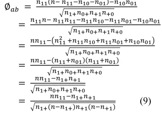
∅ . (8)
The above equation (8) is re-written to be composed of only those terms which binary values are 1s because 1 means ‘exist’;
∅
(9)
The simplified equation is used and altered for pruning non-existence titemsets. Table 4 is derived from coefficient association for two titemsets instead of two binary values. Each cell represents the possible combination of X and Y with frequency counts, sups. Non-existence called negated titem is notated with the sign ¬. Using Table 4, the equation (9) can be altered to the equation (10).
Table 4: 2ⅹ2 Contingency Table for Titemsets
Y ¬Y sum
X sup(X⇒Y) sup(X⇒¬Y) sup(X)
¬X sup(¬X⇒Y) sup(¬X⇒¬Y) sup(¬X)
sum sup(Y) sup(¬Y) 1
∅ ∙ ∪ ∙ ∙ ∙ (10)
7298 than 0.1 is not worth to be considered. The given value, 0.5, 0.3, or 0.1, called correlation threshold, is set by an input value or default value 0.5. By adopting the correlation coefficient measure, the titemsets X and Y negatively correlated and leveled more than certain reliable strength are uncovered and used to generate informative negative association rules, even in the situation where their confidence values are reasonably high, but support values are less than a given ms.
[image:6.612.93.297.236.527.2]4.3 Numerical Comparison
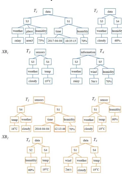
Figure 1: Tree-Structured Stream Data with 8 Trees from 2 Blocks
With respect to the simple dataset SX on Figure 1, four measures – support, confidence, interestingness, and correlation coefficient – are taken to ensure how they affect differently obtained titemsets. The example data is expressed in SX = (XB1, XB2) = ((t1, {T1, T2, T3, T4}), (t2, {T1, T2, T3T4})) and according to the equation (4), a size of SX is |SX| = 8. From the set SX, the fraction set F is configured with many fractions F.
First, when a threshold for the support, ms, is assumed ms = 0.2 and applied to each fraction F
F, it is designated by sup(F) ms which indicates only the fraction F, which occurring count is more than 1.6 (80.2) is eligible to be a titem for
generating rules. Based on the given ms, four titems from F satisfying the condition are presented on Figure 2 and three possible positive association rules are suggested on Figure 3.
Figure 2: Four Titems Satisfying a given ms
Figure 3: Three Possible Association Rules
The support-confidence measure is taken to each rule and the computational results are
(a) 𝑠𝑢 𝑝 𝑋 ⇒ 𝑌 0.375 𝑐𝑜𝑛𝑓 𝑋 𝑌 0.6, (b) 𝑠𝑢 𝑝 𝑋 ⇒ 𝑌 0.25
𝑐𝑜𝑛𝑓 𝑋 𝑌 0.4,
(c) 𝑠𝑢 𝑝 𝑋 ⇒ 𝑌 0.125 𝑐𝑜𝑛𝑓 𝑋 𝑌 0.2.
Assumed anther threshold, the minimum confidence mc = 0.5, only timesets X and Y on (a) are survived. The others are pruned. When we calculate the support-confidence again with the negated Y, ¬Y, however, the results are different;
(a) sup 𝑋 ⇒ 𝑌 0.25 𝑐𝑜𝑛𝑓 𝑋 𝑌 0.4, (b) sup 𝑋 ⇒ 𝑌 0.375
𝑐𝑜𝑛𝑓 𝑋 𝑌 0.6, (c) sup 𝑋 ⇒ 𝑌 0.5
𝑐𝑜𝑛𝑓 𝑋 𝑌 0.8.
7299 potentially valuable titemsets no matter frequency is high or not, that is the aim of this work. We take the interestingness and correlation coefficient for the purpose.
Given minimum interest mi = 0.3 and the equation (7), we compute each value of interestingness for original possible positive association forms and their negative forms in the following;
a 𝑖𝑛𝑡𝑒𝑟𝑒𝑠𝑡 𝑋 ⇒ 𝑌 ∙ 0.062 (b) 𝑖𝑛𝑡𝑒𝑟𝑒𝑠𝑡 𝑋 ⇒ 𝑌 ∙ 0.0156 (c) 𝑖𝑛𝑡𝑒𝑟𝑒𝑠𝑡 𝑋 ⇒ 𝑌 ∙ 0.109
(a’) 𝑖𝑛𝑡𝑒𝑟𝑒𝑠𝑡 𝑋 ⇒ 𝑌 ∙ 0.6875
(b’) 𝑖𝑛𝑡𝑒𝑟𝑒𝑠𝑡 𝑋 ⇒ 𝑌 ∙ 0.484
(c’) 𝑖𝑛𝑡𝑒𝑟𝑒𝑠𝑡 𝑋 ⇒ 𝑌 ∙ 0.359
It can be known that the interestingness values for the positive rules are comparatively small and all of them do not satisfy the given mi. On the other hand, the values of all the negative rules are sufficiently high which means the rules must be mined because they have important information. Such result cannot be derived by the support-confidence approach. Some rules can have high interest values even though they have not sufficient support nor confidence. But, it depends on how properly set up mi to find suitable titemsets for useful and usable association rules. Therefore, we lastly determine the negative rules throughout interestingness how strongly two titemsets are related each other according to the equation (9).
(a) ∅ ⇒
∙ ∙
∙ ∙ ∙ √ 0.258 ,
(b) ∅ ⇒
∙ ∙
∙ ∙ ∙ 0.07,
(c) ∅ ⇒
∙ ∙
∙ ∙ ∙ 0.47 .
With respect to the strength of correlation coefficient explained in the previous, it can be informed that the case (b) is not worth to be considered because its value is less than +0.1, which means two titemsets are nearly independent each other and the association between them is seldom made. In other measures, it has been determined as a frequently occurred but less reliable rule by the support/confidence and it has been determined as a not interesting rule by the interestingness. And, it is
determined as a rarely related rule between titemsets by the coefficient. Concerning the coefficient determination, the rule (c) on the figure 3 has the strong negative association between titesmsets and its interesting value is reasonable to be mined even though its support value is less than the given ms.
Applying two measures, interestingness and correlation coefficient values, indicate that 1) the rules have negative relationship between titemsets, 2) the strengths of their coefficients are quite strong enough to give valuable information, and 3) the generated negative association rule will provide many opportunities for further mining, even though their support values are less than ms and the rules are not attracted in the positive versions. With the frame of correlation coefficient, the hidden association of (c) provides benefits when it is mined for a negative association rule, which is not caught by support/confidence or even interest.
4.4 Frame Algorithm DNTS
The following algorithm DNTS determines the way how to apply 4 measuring factors and discover valuable negated titemsets. Table 5 summarizes all thresholds and their abbreviations or statistical levels used in the algorithm.
Algorithm DNTS
INP: XDS OUTP: NTS
1. FOR EACH block XBi∈XDS (1
i
k)2. FOR j ← 1 to n
3. IF freq(Xij, XDS)
|XDS|
4. THEN FT = FT + { Xij };
5. FOR titemset X
FT, Y
FT, X
Y = 0 6. IF sup (X⇒Y) < ms 7. or conf (X⇒Y) < mc8. THEN
9. IF interest(X, ¬Y) < mi
10. THEN
11. IF
(X, ¬Y)
−0.3 or
(X, ¬Y)
+0.3 12. THEN NTS ← NTS + {X⇒ ¬Y}; 13. ELSE14. THEN NTS ← NTS + {X⇒ ¬Y}; 15. ELSE
16. THEN NTS ← NTS + {X⇒ ¬Y}; 17. RERURN NTS
7300
Table 5: Thresholds Used by DNTS Algorithm
Threshold Abbr. / Level Strength minimum
support ms NA
minimum
confidence mc NA
minimum
interest mi NA
correlation coefficient value
0.1 no association
03 moderate association
0.5 strong association
With the given dataset on Figure 1 and running the algorithm, a line 3 and equations (4), (5) manage total 8 xml trees in 2 blocks with an assumed minimum frequency threshold, = 0.2. The first condition indicates that only titems which occurrence counts are more than 1.6 (80.2) are included in the set FT. We select two rules on Figure 4 to present the importance of finding negated titems and show how the algorithm works for it. Each titem
X and Y on satisfies the frequency condition. As stated in lines 5 to 7, an ordinary form X ⇒ Y is concerned. Its sup(X ⇒ Y) and conf (X ⇒ Y) are computed according to the previously defined formulas [12], 1/8 0.125 and 1/5 0.2 , respectively. Because the rule (a) does not satisfy two conditions, it must be pruned. However, the suggested algorithm is not. By the line 9, the body Y
is negated and interest(X, ¬Y) is computed according to the equation (6); ∙ 0.359. Since the rule X ⇒ ¬Y is interest or not depends on mi, we apply (X, ¬Y) for a clear output. By the equation (7),
(X, ¬Y) =
∙ ∙
∙ ∙ ∙ 0.47.
Figure 4: Association Rules with or without Negated Y
According to Table 5 the produced value is close to − 0.5 which indicates the strong association. The temporal rule (a) is not a valuable positive association rule, but the rule (b) is an interesting and valuable negative association rule generated from (a). A correlation coefficient value indicates that 1) a rule
has negative or positive relationship between titemsets by the sign, 2) how strongly two titemsets are associated each other, and 3) it makes up for the weak point of the other three factors.
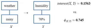
Another simple example is provided on Figure 5 for better understanding the differentiation between interest determination and correlation coefficient determination. With respect to the dataset on Figure 1, the obtained support and confidence values of the given rule are 0.25 and 1, respectively. When we assume ms = 0.3, the association between
X and Y does not satisfy the condition and is pruned from association rule generation, even though two titemsets have the strong tandem. Under the support/confidence framework, there is no chance to consider them. Thus, we add the factor interest to determine its interestingness. When the given mi is 0.3, the candidate rule is still pruned because it is determined as ‘uninteresting’. The rule could be interest to be mined if mi would be set less than 0.15. The determination of interestingness is highly dependable on setting up mi. But, the value of correlation coefficient gives a more objective result. Its obtained value is approximately 0.75, which means there is a strong positive correlation between
[image:8.612.320.507.477.535.2]X and Y and cannot be ignored. As proved by the confidence value, the titemset Y always occurs if the titemset X occurs. Concerning the coefficient determination, the example rule is decided to have helpful information even though its support value is less than ms.
Figure 5: Different Results of interestingness vs. correlation coefficient value
5. CONCLUSION
7301 added some measures were suggested as the alternatives; interestingness and correlation coefficient. We adjusted both measures for our data to determine non-existing but important titemsets. The example results of interestingness and correlation coefficient were presented and compared with a few illustrations based on the algorithm DNTS. We drew out it would be more efficient and reliable to prune fractions with the correlation determination than that of interestingness, too. We presented for the first time the analyses of both interestingness and correlation coefficient methods over tree structured stream data. Future work includes presenting a full mining algorithm and experimental results of negative association rules for tree structured stream data that is proven to work with the four measurements.
REFRENCES:
[1] M. Botts, G. Percivall, C. Reed, and J. Davidson, “OCG® Sensor Web Enablement: Overview and High Level Architecture”, Proceedings of the 2nd International Conference on GeoSensor Networks, October 1-3, 2006, USA, LNCS 4540, pp. 175-190.
[2] A. Bröring, J. Echterhoff, S. Jirka, I. Simonis, T. Everding, C. StSCH, s. Kiang, and R. Lemmens, “New Generation Sensor Web Enablement”, Sensors 2011, 11, pp. 2652-2699.
[3] S. Mahmood, M.Shahbaz, and A. Guergachi, “Negative and Positive Association Rule Mining from Text Using Frequent and Infrequent Itemsets”, The Scientific World Journal, Vol. 2014, ID 973750, 2014, 11 pages.
[4] K.K. Loo, I. Tong, B. Kao, and D. Chenung, “Online Algorithms for Mining Inter-Stream Associations from Large Sensor Networks”, Advances in Knowledge Discovery and Data Mining, Proceedings of the 9th Pacific-Asia Conference on Knowledge Discovery and Data Mining, May 18-20, 2005, Vietnam, LNCS 3518, pp. 143-149.
[5] A. Savasere, E. Omiecinski, and S. Navathe, “Mining for Strong Negative Associations in a Large Database of Customer Transactions”, Proceedings of the 14th International Conference on Data Engineering, February 23-27, 1998, USA, pp. 494-502.
[6] M. L. Antonie and O. R. Zaïane, “Mining Positive and Negative Association Rules: An Approach for Confined Rules”, Proceedings of the 8th European Conference on Principles and Practice of Knowledge Discovery in Databases,
September 20-24, 2004, Italy, LNCS 3202, pp. 27-38.
[7] Z. Honglei and X. Zhigang, “An Effective Algorithm for Mining Positive and Negative Association Rules”, Proceedings of International Conference on Computer Science and Software Engineering, December 12-14, 2008, China, pp. 455-458.
[8] R. Sumalatha and B. Ramasubbareddy, “Mining Positive and Negative Association Rules”, International Journal on Computer Science and Engineering, Vol. 2, No. 09, 2010, pp. 2916-2910.
[9] X. Wu, C. Zhang, and S. Zhang, “Efficient Mining of Both Positive and Negative Association Rules”, ACM Transaction on Information Systems, Vol. 22, No. 03, 2004, pp. 381-405. [10] W. Ouyang, “Mining Positive and Negative
Association Rules in Data Streams with a Sliding Window”, Proceedings of the Fourth Global Congress on Intelligent Systems, December 3-4, 2013, Hong Kong, pp. 205-209.
[11] S. Corpinar and T. Í. Gündem, “Positive and Negative Association Rule Mining on XML Data Streams in Database as a Service Concept”, Expert Systems with Applications, Vol. 39, No. 8, 2012, pp. 7503-7511.
[12] J. Paik, J. Nam, U. Kim, and D. Won, “Association Rule Extraction from XML Stream Data for Wireless Sensor Networks”, Sensors, Vol. 14, 2014, pp. 12937-12957.
[13] X. Yuan, B. P. Buckles, Z. Yuan, and J. Zhang, “Mining Negative Association Rules”, Proceedings of the 7th International Symposium on Computers and Communications, July 1-4, 2002, Italy, pp. 623-628.
[14] R. Agrawal, T. Imieliński, and A. Swami, “Mining Association Rules Between Sets of Items in Large Databases”, Proceedings of the ACM SIGMOD international conference on Management of Data, May 25-28, 1993, USA, pp. 207-216.
[15] D. Braga, A. Campi, S. Ceri, M. Klemettinen, and P. L. Lanzi, “A Tool for Extracting XML Association Rules”, Proceedings of the 14th IEEE International Conference on Tools with artificial Intelligence, November 4-6, 2002, USA, pp. 57-64.
7302 [17] L. Feng and T. Dillon, “Mining Interesting
XML-Enabled Association Rules with Templates”, Proceedings of the 3rd International Workshop on Knowledge Discovery and Inductive Databases, September 20, 2004, Italy, LNCS 3377, pp. 66-88.
[18] L. Geng and H. J. Hamilton, “Interestingness Measures for Data Mining: A Survey”, ACM Computing Survey, Vol. 38, No. 1, 2006, article no. 9.
[19] G. Piatetsky-Shapiro, “Discovery, Analysis, and Presentation of Strong Rules”, Knowledge Discovery in Databases, Edited G. Piatetsky-Shapiro and W. J. Frawley, AAAI Press, 1991, pp.229-248.
[20] J. Cohrn, “Statistical Power Analysis for the Behavioral Sciences”, Lawrence Erlbaum), New Jersey, 1988, pp.109-143.
[21] W. Hopkins, “A New View of Statistics”,
Electronic edition, Available: