GENETIC NETWORK PROGRAMMING REINFORCEMENT LEARNING BASED SAFE AND SMOOTH MOBILE ROBOT NAVIGATION IN UNKNOWN DYNAMIC ENVIRONMENTS

IMPROVING TRANSIENT PERFORMANCES OF VEHICLE

YAW RATE RESPONSE USING COMPOSITE NONLINEAR

FEEDBACK

1_{M.K ARIPIN,} 2_{Y.M SAM,} 3_{KUMERESAN A.D,} 4_{M.H CHE HASAN,} 5_{M.FAHEZAL ISMAIL}

1

Senior Lecturer. Universiti Teknikal Malaysia Melaka, Centre for Robotics & Industrial Automation,

Faculty of Electrical Engineering, Malaysia 2

Professor. Universiti Teknologi Malaysia, Department of Control & Mechatronics, Faculty of Electrical

Engineering, Makaysia 3

Senior Lecturer. Universiti Teknologi Malaysia, Department of Control & Mechatronics, Faculty of

Electrical Engineering, Makaysia 4

Senior Lecturer. Universiti Teknikal Malaysia Melaka, Centre for Robotics & Industrial Automation,

Faculty of Engineering Technology, Malaysia 5

Senior Lecturer. Universiti Kuala Lumpur Malaysia France Institute, Industrial Automation Section,

Malaysia

E-mail: [email protected], [email protected], [email protected], 4

[email protected], [email protected]

ABSTRACT

This paper studies and applied the composite nonlinear feedback (CNF) control technique for improving the transient performances of vehicle yaw rate response. In the active front steering control design and analysis, the linear bicycle model is used for controller design while the 7DOF nonlinear vehicle model is used as vehicle plant for simulation and controller evaluations. The vehicle handling test of the J-turn and single lane change maneuvers are implemented in computer simulations in order to evaluate the designed yaw rate tracking controller. The simulation results show that the CNF technique could improve the transient performances of yaw rate response and enhance the vehicle maneuverability.

Keywords: Composite Nonlinear Feedback, Yaw Rate Response, Active Front Steering Control, Vehicle Yaw Stability, Lateral Dynamic Control

1. INTRODUCTION

In lateral dynamic control of front wheel steer vehicle such as car passenger, the yaw stability control system is one of the prominent approaches to improve the vehicle handling and stability especially during low to mid-range of lateral acceleration. To ensure the lateral stability, it is important to control the vehicle yaw rate where this variable is closely related to the front wheel steer angle. The actual yaw rate response must be tracked and close to yaw rate desired response which generated by a yaw rate reference model. In order to realize this tracking control task, an active front steering (AFS) control can be implemented. The proposed controller will generates the corrective

steer angle and adding to driver’s steer angle as a front wheel steer angle to the vehicle.

algorithm used to improve the handling and stability of AFS control is model predictive control (MPC) as presented in [6], optimal control theory in [7] and linear quadratic regulator (LQR) in [8]. To cater the uncertainties of vehicle parameters and disturbances, a few of robust control algorithms are implemented for AFS control. As reported in [9], the Mu-control theory is adapted as robust yaw rate controller in variations of vehicle loading, road surface conditions and external disturbances. Another robust control algorithm applied for yaw rate controller is quantitative feedback control theory (QFT) as discussed in [10]. In this study, variations of the vehicle mass, velocity and road surface conditions are considered as uncertainty parameters. Recently, and adaptive sliding mode control based on integral sliding surface is designed to cater the uncertainties and disturbances in [11]. In this AFS control design, the yaw controller improves the handling and path tracking performances.

From the control system point of view, the performances of transient response are very important in tracking control. For most practical situation, it is desired to obtain a fast response with small overshoot, but in fact, most of control scheme makes a trade-off between these two transient performance parameters. In the research works above, it is observed that the improvement of transient performance parameters such as transient time, settling time and percent overshoot is not well emphasized. The proposed control strategies are not accommodated for transient response improvement of the yaw rate response. Therefore, this inadequacy in AFS control has initiated a motivation to propose an appropriate control technique for this purpose.

The composite nonlinear feedback (CNF) is one of the control technique that developed based on the state feedback law. This control technique is proven in order to improve the transient performances as designed and implemented in [12] for tracking control of linear system and multivariable constrained input linear system in [13]. It was extended and designed for linear system with input saturation in [14], general multivariable system with input saturation [15], hard disk drive system servo system [16, 17], servo positioning system [18, 19], nonlinear system with input saturation [20], and continually developed and applied in the last decade. In the vehicle dynamics studies, a research work in [21] has successfully applied the CNF technique for quarter car active suspension system. In this study, the performances of ride comfort and road handling is improved.

The CNF control technique is working based on variable damping ratio concept. During the transient period, the damping ratio is kept at low level and when the output response closer to the reference set point, the CNF varies the damping ratio to high level. In general, the CNF control technique is designed in three important steps. The first one is design the linear feedback control law with small damping ratio to achieve fast response with faster rise time in a closed loop system. In the second step, the nonlinear feedback law is designed by increasing the damping ratio to achieve desired response at very minimum overshoot. Then, the linear and nonlinear feedback control laws are combined in the final step without any switching element as a complete CNF control law.

From the above discussion, an advantages of the CNF in improving the transient performances is considered for AFS control in order to track the desired yaw rate response. In our previous work [22], the CNF is applied as yaw rate tracking controller for AFS control and the proposed controller is evaluated using the J-turn handling test only. In this paper, we extended the controller evaluation for another handling test, i.e. single lane change maneuver. The controller evaluation is performed in the computer simulations using the Matlab/Simulink software. The linear bicycle model and nonlinear vehicle model are utilized for the controller design and vehicle plant respectively.

This section had discussed an overview of AFS control, existing yaw control strategies and the principle of the CNF control technique. Section 2 of this paper will discuss the dynamics of the nonlinear vehicle model and a linear bicycle model. The design procedures of CNF control technique are detailed in Section 3 while Section 4 presented the simulation results and discussion. Finally, Section 5 provides a conclusion and future works.

2. VEHICLE DYNAMICS MODEL

2.1 Nonlinear Vehicle Model for Simulation

The nonlinear 7DOF vehicle model in planar motion as depicted in Figure 1 is used to represent as vehicle plant. The dynamics for forward vehicle speed (longitudinal motion), sideslip (lateral motion) and yaw rate (yaw motion) which form 3DOF are described in (1), (2) and (3) respectively; ] sin ) ( ) sin( ) ( cos ) ( ) cos( ) [( 1 4 3 2 1 4 3 2 1 β δ β β δ β y y f y y x x f x x F F F F F F F F m v + + − + + + + − + = & (1) r F F F F F F F F mv y y f y y x x f x x − + + − + + + − − + − = ] cos ) ( ) cos( ) ( sin ) ( ) sin( ) ( [ 1 4 3 2 1 4 3 2 1 β β δ β δ β β& (2) ) ( ) cos sin 2 ( ) cos sin 2 ( ) ( 2 ) cos 2 sin ( ) cos 2 sin ( [ 1 4 3 2 1 4 3 2 1 y y r f f f y f f f y x x f f f x f f f x z F F l l d F l d F F F d d l F d l F I r + − + − + + + − + + + − = δ δ δ δ δ δ δ δ & (3) d 2 x F 2 y F 1 y F 1 x F 4 x F 3 x F 4 y F 3 y F x v v r d

β lf

r l

y

v Mz

f

δ δf

Figure 1: Nonlinear Vehicle Model

The vehicle parameters involved in (1) - (3) above are described in Table 1 and the values are taken from [23]. The input variable to the model is front wheel steer angle δf while the yaw rate r

is the output or control variable. The nonlinear longitudinal tire forces F_xi and lateral tire forces

yi

F are described using the nonlinear tire model which will discuss later. The subscript i is wheel number, i.e. 1 for front-left, 2 for front-right, 3 for rear-left and 4 for rear-right while the vehicle speed

vis always assumed at a constant value.

Table 1: Vehicle Parameters

Symbol Description Value/Unit

m vehicle mass 1704.7 kg

lf distance from front axle to centre of gravity

1.035m

lr distance from rear axle to centre of gravity

1.655m

d width track 1.54m

Iz moment of inertia 3048.1kgm2

Cf front tire cornering stiffness 105,800N

Cr rear tire cornering stiffness 79,000N

2.2 Tire Dynamics Model

In vehicle dynamics studies, each wheel represents 1DOF. Thus, there are 4DOF for road vehicle with 4 wheels. The dynamic motion for each wheel is described as follows

bi ei xi wi i

wi R F T T

I ω& =− + − (4) where I_wi is wheel inertia,ω_i is wheel angular acceleration,R_wiis wheel radius, T_ei is driving torque and T_bi is braking torque. The nonlinear longitudinal tire forces F_xi and lateral tire forces

yi

F in (1) - (3) are depending on the tire slip angles α_i, tire longitudinal slip λ_i, road surface adhesion coefficientµand tire normal forces Fzi.

These nonlinear tire forces can be described using the Pacejka tire model [24] as shown in the following equations

[

tan ( . ( . tan ( . )))

]

sin xi 1 xi i xi xi i 1 xi i xi

xi D C B E B B

F = − λ − λ − − λ (5)

[

tan ( . ( . tan ( . )))

]

sin _yi 1 _{yi f yi yi f} 1 _{yi f} yi

yi D C B E B B

The D, C, B and E parameters in the above equations are known as tire model parameters. Table 2 shows the tire model parameters that used in this paper.

Table 2: Pacejka Model Parameters

Front/ Rear Tire Lateral/ longitudinal forces Parameters Value Front tire

lateral By=9.094 Cy=1.193 Dy=-4.876 Ey=-1.252

longitudinal Bx=11.39 Cx=1.685 Dx=6164 Ex=0.3694

Rear tire

lateral By=10.11 Cy=1.193 Dy=-3273 Ey=-0.972

longitudinal Bx=10.01 Cx=1.685 Dx=3912 Ex=0.3246

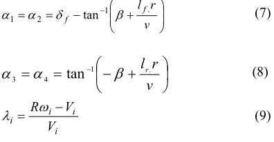
The tire sides slip angle and longitudinal wheels slip in (5) and (6) above are computed as follows         + − = = − v r l_f f . 1 2

1 α δ tan β

α (7)













₋

₊

=

=

−

v

r

l

r. 1

4

3

α

tan

β

α

(8)

i i i i V V R − = ω

λ (9)

where V_i in (9) above is the ground contact speed of each wheel as given in the following equations;

      − −

= lfβ

d r v V

2

1

(10)

      + +

= lfβ

d r v V

2

2 (11)

      − −

= lrβ

d r v V

2

3 (12)

      − +

= lrβ

d r v V

2

4

(13)

Tire normal forces Fzi or so called wheel vertical

load during constant speed that essential for tire force calculation can be obtained using the following equations         − + − + = d ha l l ha l l gl m F y r f x r f r z 2

1 (14)

        − + − + = d ha l l ha l l gl m F y r f x r f r z 2

2 (15)

        − + + + = d ha l l ha l l gl m F y r f x r f f z 2

3 (16)

        + + + + = d ha l l ha l l gl m F y r f x r f f z 2

4 (17

)

where h is the height of the centre of gravity (CG),

y

a is lateral acceleration, a_x is longitudinal acceleration, g is gravitational constant, lf,lr and

d are vehicle parameters as discussed above.

2.3 Linear Vehicle Model for Controller Design

The classical linear bicycle model in Figure 2 is used to design the yaw rate tracking controller of AFS control. Based on a few assumptions as discussed in [25], this bicycle model consists of 2 DOF i.e. lateral and yaw motions with the tire forces are operated in the linear region. f l r l r yf F v

β δf

[image:4.612.90.288.346.449.2]

y f α r α yr F

Figure 2: Linear Bicycle Model

The dynamics of vehicle sideslip β (lateral motion) and yaw rate r (yaw motion) are described as follows

yr yf

F

F

r

mv

(

β

&

+

)

=

+

(18)

yr r yf f

zr l F l F

I &= − (19)

where m,lf,lr and Iz are vehicle parameters as described in Table 1 while the vehicle speed v is constant. The front lateral tire force Fyf and rear

lateral tire force Fyr are in a linear relationship

with tire slip angle as described in the following equations

f f

yf C

F =

α

(20)

r r

yr C

[image:4.612.314.492.411.456.2]

where Cf and Cr are cornering stiffness for front

and rear tire respectively. Front and rear tire slip angle, αf and

α

rfor linear tire force are given as follows

v r l_f

f

f =δ −β−

α

(22)

v r

l_r

r =−

β

+

α

(23)

By substituting and simplify (18) – (23), a linear state space equation of bicycle model is obtained as follows

f

z f f

f

z r r f f

z f f r r

f f r r r

f

I l C

mv C r v I

l C l C I

l C l C

mv l C l C mv

C C

r Bu Ax x

δ β

β

   

 

   

 

+      

   

 

   

 

− − −

− + − − −

=      

+ =

2 2

2 1

& & &

(24)

2.4 Reference Model

The control objective of active front steering control is to track and bring the actual vehicle yaw rate response close to the desired response. The desired yaw rate response is highly related to the front wheel steering angle δf and

vehicle speed v. In steady state condition, the desired yaw rate rd is described as follows

f u d

v k l

v

r ₂.δ

+

=

(25)

where k_u is cornering stability factor and given by the following equation

r f r f

f f r r u

C C l l

C l C l m k

) (

) (

+ −

=

(26)

However, the steady state yaw rate r_ssis limited due to lateral acceleration of the vehicle in g unit could not exceed the maximum road friction coefficientµ. The limited value of r_ss is given in the following equation

v g

r_ss ≤

µ

(27)

3. COMPOSITE NONLINEAR FEEDBACK

CONTROL TECHNIQUE

The CNF control technique could be designed and applied to the system with or without external disturbances. In this paper, we considered that the vehicle dynamic plant is without an external disturbance and all the states can be measured. This section will discuss the design procedures, parameters tuning, and stability analysis of yaw rate tracking controller using the CNF technique.

3.1 The CNF Design Procedures

In general, the CNF is designed based on linear time-invariant continuous system with input saturation as follows

Cx y

x x u Bsat Ax

x _o

=

= +

= ( ) (0)

&

(28)

where A, B and C are system, input and output matrices respectively, with an appropriate dimension. The matrices (A,B) are assumed controllable, matrices (A,C) are assumed observable and matrices (A,B,C) is assumed invertible and has no zero at s=0. The input saturation is defined as

{

u u

}

u u

sat( )=sgn( )min _max,

(29)

where u_max is the saturation level of the input. As established in [14], the CNF control laws are designed in three important steps as follows

1) design a linear feedback control law, Gr

Fx

uL= + (30)

2) design a nonlinear feedback control law

,

) ( ) ,

( _e

N r y BP x x

u =ρ ′ −

(31)

3) completed the CNF control law,

L

N u

u

u= + (32)

In step 1, F is feedback gain matrix so that A+BF is an asymptotically stable and closed loop system

B BF A sI

C( − − )−1 has a small damping ratio while scalar G is defined as follows

[

₁

]

1

)

( + − −

−

= C A BF B

In step 2, the ρ(r,y) is nonpositive function locally Lipschitz in y which is used to vary the closed loop damping ratio as output approaches the step command input. The P>0is the solution of following Lyapunov equation

W BF A P P BF

A+ )′ +( ( + )=−

(

(34)

for some given W >0and xeis given as

r BG BF A

x_e =[−( + )−1 ]

(35)

The nonlinear function ρ(r,y) is not unique where

the variety of choices can be used as stated in [26]. To adapt the tracking control task, the nonlinear function used in [27, 28] is utilized in this paper which is described in the following equation

r y

o e y

r =−γ ϕϕ −

ρ( , )

(36)

where

   

= ≠ −

=

r y

r y r y

o o o

o

, 1

, 1

ϕ

(37)

3.2 Tuning Parameters of CNF

The tuning of design parameters in nonlinear function of CNF control design is essential so that the controlled output approaches the reference set point. The tuning is based on desired steady state damping ratio, IAE and ITAE criteria as implemented in [28] which is summarized as follows

i) choose the desired steady state damping ratio

ss

ξ

ii) determine

γ

by letting the steady state system has a damping ratio of ξ_ss

iii) determine an optimal

ϕ

by solving minimization some appreciable criteria of IAE and ITAE which given by the following equation

dt e

∫

∞

0

min_ϕ or

∫

tedt

∞

0

min_ϕ

(38)

where e= y−r is yaw rate tracking error.

3.3 Yaw Rate Tracking Controller based CNF

The yaw rate tracking controller of AFS control using the CNF technique is illustrated in Figure 3. The actual yaw rate from the nonlinear vehicle model is fed back into the controller. By using the yaw rate tracking error information, the

CNF is generated the corrective steer angle,δ_c and

added with driver steer angle δfd as a front wheel

steer angle δf to the vehicle i.e. δf =δfd+δc.

Based on vehicle parameters and the CNF design procedures as above, the linear state space model for controller design, desired yaw rate and the CNF control parameters are obtained as follows

Linear state space model:

f

r

r δ

β β

      +          

 

− − −

=      

925 . 35

2343 . 2 8942

. 3 9689 . 6

9839 . 0 9026 . 3

& &

Desired yaw rate: rd =7.0654δf

CNF parameters:

[

]

03 . 0 , 2 . 0

1 1711 . 0 ,

1535 . 0 0562 . 0

0562 . 0 8224 . 0

2321 . 0 , 05 . 0 5 . 0

= =

   

 − =    

  =

= −

=

ϕ

γ

e

G P

G F

3.4 Stability Analysis

The stability analysis of AFS control closed loop system as shown in Figure 3 above is determined by using a Lyapunov stability theory. The closed loop system of the plant described in (28) and linear control law in (30) is given as follows

BHr Ax x BF Ax

x =[ + ]~+ _e+

~_&

₍₃₉₎

By proof that termAx_e+BHr=0, hence

linear closed loop system is simplified as follows

x BF Ax

x [ ]~

With linear and nonlinear control laws of the CNF in (32), the closed loop system for plant in (28) is expressed as

ϑ

B x BF Ax

x =[ + ]~+

~_&

₍₄₁₎

By using Lyapunov functionV =x~TP~x,

the time derivative of Lyapunov function along the close system trajectories of the equation (41) is obtained as follows

e

x x

x = −

~

₍₄₂₎

and

Hr x F u Hr x F

sat + + _N − −

= ₍ ~ ₎ ~

ϑ

(43)

By using Lyapunov function V =x~TP~x, the time

derivative of Lyapunov function along the close system trajectories of the equation (41) is obtained as follows

[

]

[

]

ϑ

ϑ

PB x x W x V

PB x x BF A P x x P BF A x V

x P x x P x V

T T

T T

T T

T T

~ 2 ~ ~

~ 2 ~ ~

~ ~

~ ~ ~ ~

+ − =

+ + + +

= + =

& &

& &

&

(44)

For case when F~x+Hr+u_N ≤u_max, then

x BTP

u_N ρ ~

ϑ= = . Hence, V&is calculated as

x W x x P PBB x x W x

V&=−~T ~+2ρ~T T ~≤−~T ~

(45)

For case when F~x+Hr+uN >umax, then

x P B u Hr x F

u ~ _N T ~

0<ω= _max − − < =ρ which

implies that ~xTPB<0. Hence, V&is calculated as

x TW x TPB x x TW x

V& =−~ ~+2~ ω≤−~ ~

(46)

For case when F~x+Hr+u_N <−u_max, then

0 ~

~

max− − <

− = <

=u u Fx Hr x

P

BT _N ω

ρ which

implies that ~xTPB>0. Hence, V&is calculated as

x W x

V& ≤−~T ~ (47)

In general, all trajectories of closed loop system in equation (40) will converge to origin for

all condition stated in equation (47) with W >0.

4. SIMULATION RESULTS

The simulation is performed using Matlab/Simulink software. In our previous work [22], only J-turn manouevre test is conducted. In this paper, the J-turn and single lane change manoeuvres are implemented to evaluate the propose controller.

4.1 J-turn Maneuver

The simulation is performed using Matlab/Simulink software. The road surface adhesion coefficient is considered for an ideal road

surface i.e. µ=1and vehicle speed, v is constant at

100 km/h.

The J-turn cornering manoeuvre which is similar to the step input test is one of vehicle handling tests to examine the transient and steady state performances of yaw stability control. As implemented in [22], the driver’s steer input is only at 1 of steer angle. In this paper, the controller is ο

evaluated with 2.5οsteer angle as shown in Figure

4 which is considered will generate an appropriate level of lateral acceleration. The yaw rate response with the CNF is compared to uncontrolled and the classical PID controller, which tuned by the Matlab PID control toolbox. Figure 5 and 6 shows the yaw rate response and yaw rate tracking error respectively.

0 1 2 3 4 5 6 7 8

0 0.5 1 1.5 2 2.5

time (sec)

s

te

e

ri

n

g

a

n

g

le

(

d

e

g

)

J-turn steer input

0 1 2 3 4 5 6 7 8 0

2 4 6 8 10 12 14 16 18 20

X: 6.587 Y: 17.65

Time (s)

Y

a

w

r

a

te

(

d

e

g

/s

)

yaw rate response

Reference uncontrolled vehicle AFS control based PID AFS control based CNF

1.2 1.4 1.6 1.8 2 2.2 2.42.6 10

[image:8.612.94.297.77.248.2]

12 14 16 18

Figure 5: Yaw Rate Response of J-Turn Maneuver

0 1 2 3 4 5 6 7 8

-1 0 1 2 3 4 5 6

Time (s)

T

ra

c

k

in

g

E

rr

o

r

(d

e

g

)

yaw rate tracking error

uncontrolled vehicle AFS control based PID AFS control based CNF

0.5 1 1.5 2 0

1 2 3

Figure 6: Yaw Rate Tracking Error of J-Turn Maneuver

[image:8.612.331.517.232.354.2]

From Figure 5, it is observed that the CNF could track the yaw rate desired response with better transient performances compared to PID an uncontrolled vehicle. As tabulated in Table 3, there is no overshoot, faster rise time and settling time for yaw rate response with the CNF. In terms of yaw rate tracking error, the yaw rate response with the CNF has smallest error compared to PID controller and uncontrolled vehicle as shown in Figure 6. This means that CNF control could track the reference response as close as desired.

Table 3: Transient Parameters of J-turn Maneuver

Controller _Mp %OS _{tr (s) ts (s)}

uncontrolled 17.6 11.08% 0.458s 3.42s

PID 18.12 12.72% 0.403s 3.37s

CNF nil 0% 0.388s 3.21s

4.2 Single Lane Change Maneuver

The single lane change (SLC) maneuver is one of the sinusoidal input tests to analyse the yaw rate tracking performances. Variable amplitude of sinusoidal signal will produce lateral acceleration from low level to peak level. Figure 7 shows the sinusoidal waveform with 0.5Hz frequency and

ο

5 .

2 maximum amplitude to represent a SLC steer

input.

0 1 2 3 4 5 6 7 8

-2.5 -2 -1.5 -1 -0.5 0 0.5 1 1.5 2 2.5

time(sec)

s

te

e

ri

n

g

a

n

g

le

(

d

e

g

)

Single lane change steer input

Figure 7: SLC Steer Input at 2.5ο Maximum Amplitude.

0 1 2 3 4 5 6 7 8

-20 -15 -10 -5 0 5 10 15 20

Time (s)

Y

a

w

r

a

te

(

d

e

g

/s

)

yaw rate response

Reference uncontrolled vehicle AFS control based PID AFS control based CNF

1.21.4 1.6 1.8 2 2.2 2.4 2.6 5

[image:8.612.113.295.282.448.2]

10 15 20

Figure 8: Yaw Rate Response of SLC Maneuver

0 1 2 3 4 5 6 7 8

-5 -4 -3 -2 -1 0 1 2 3 4 5

Time (s)

T

ra

c

k

in

g

E

rr

o

r

(d

e

g

)

yaw rate tracking error

uncontrolled vehicle AFS control based PID AFS control based CNF

0.60.8 1 1.21.41.61.8 2 0

1 2 3 4

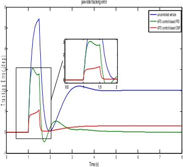
[image:8.612.334.518.391.520.2] [image:8.612.329.522.555.681.2] [image:8.612.85.305.623.696.2]

From Figure 8, the AFS control with the CNF show the better yaw rate tracking performance compared to the PID controller and uncontrolled vehicle. The yaw rate response with the CNF is close to the desired yaw rate where it is obviously observed that the yaw rate tracking error with the CNF is small compared to the PID controller and uncontrolled vehicle as shown in Figure 9.

The simulation of yaw rate tracking controller based on the CNF control technique has been presented. The yaw rate response of the AFS control with the CNF is compared and evaluated with PID controller and uncontrolled vehicle. From the responses obtained, it is demonstrated that the CNF performed the yaw rate tracking control task with better transient performances which could enhance the vehicle handling and maneuverability.

5. CONCLUSION

The composite nonlinear feedback (CNF) control is applied as a new control strategy for yaw rate tracking controller in AFS control strategy. Based on the results obtained, the CNF control technique improved the transient performances of yaw rate response with minimum overshoot, faster rise time and settling time for a J-turn cornering maneuver and excellent tracking performances in the single lane change maneuver. As a conclusion, the CNF control technique is able to enhance the vehicle lateral dynamic control and vehicle maneuverability. For future works, the CNF control technique will be integrate with robust control technique such as sliding mode control to cater an external disturbances and uncertainties of vehicle parameters

ACKNOWLEDGEMENT

The authors would like to thankful to Centre for Researh & Innovation Management (CRIM) and CeRIA, UTeM, UTM and MoHE for the present works.

REFERENCES:

[1] G. Tekin and Y. S. Ünlüsoy, "Design and simulation of an integrated active yaw control

system for road vehicles," International

Journal of Vehicle Design, vol. 52, , 2010, pp.

5-19.

[2] J. Ma, G. Liu, and J. Wang, "An AFS control based on fuzzy logic for vehicle yaw

stability," Proceedings of the 2010

International Conference on Computer

Application and System Modeling, 2010, pp.

V5503-V5506.

[3] Q. Li, G. Shi, and J. Wei, "Yaw stability control using the fuzzy PID controller for

active front steering," High Technology

Letters, vol. 16, 2010, pp. 94-98.

[4] Q. Li, G. Shi, J. Wei, and Y. Lin, "Yaw stability control of active front steering with

fractional-order PID controller," Proceedings

of the 2009 International Conference on

Information Engineering and Computer

Science, 2009, pp. 1-4.

[5] B. Zheng and S. Anwar, "Yaw stability control of a steer-by-wire equipped vehicle via

active front wheel steering," Mechatronics,

vol. 19, 2009, pp. 799-804.

[6] P. Falcone, F. Borrelli, J. Asgari, H. E. Tseng, and D. Hrovat, "Predictive active steering control for autonomous vehicle systems," IEEE Transactions on Control Systems

Technology, vol. 15, 2007, pp. 566-580.

[7] A. Goodarzi, E. Esmailzadeh, and B. Nadarkhani, "Design of an optimal control strategy for an active front steering system,"

Proceedings of the 8th Biennial ASME

Conference on Engineering Systems Design

and Analysis, 2006, pp. 313-320.

[8] W. A. H. Oraby, S. M. El-Demerdash, A. M. Selim, A. Faizz, and D. A. Crolla, "Improvement of Vehicle Lateral Dynamics

by Active Front Steering Control,"

Proceedings of the SAE Automotive

Dynamics, Stability & Controls Conference

and Exhibition (Michigan), 2004, SAE

2004-01-2081.

[9] C. C. Yuan, L. Chen, S. H. Wang, and H. B. Jiang, "Robust active front steering control

based on the Mu control theory," Proceedings

of the 2010 International Conference on

Electrical and Control Engineering, 2010, pp.

1827-1829.

[10] J. Y. Zhang, J. W. Kim, K. B. Lee, and Y. B. Kim, "Development of an active front steering

(AFS) system with QFT control,"

International Journal of Automotive

Technology, vol. 9, 2008, pp. 695-702.

[11] D. V. Thang Truong and W. Tomaske, "Active front steering system using adaptive

sliding mode control," Proceedings of the 25th

Chinese Control and Decision Conference,

2013, pp. 253-258.

International Journal of Control, vol. 70, 1998, pp. 1-11.

[13] M. C. Turner, I. Postlethwaite, and D. J. Walker, "Non-linear tracking control for

multivariable constrained input linear

systems," International Journal of Control,

vol. 73, 2000, pp. 1160-1172.

[14] B. M. Chen, T. H. Lee, K. Peng, and V.

Venkataramanan, "Composite nonlinear

feedback control for linear systems with input

saturation: Theory and an application," IEEE

Transactions on Automatic Control, vol. 48,

2003, pp. 427-439.

[15] Y. He, B. M. Chen, and C. Wu, "Composite nonlinear control with state and measurement feedback for general multivariable systems

with input saturation," Systems and Control

Letters, vol. 54, 2005, pp. 455-469.

[16] K. Peng, B. M. Chen, G. Cheng, and T. H.

Lee, "Modeling and compensation of

nonlinearities and friction in a micro hard disk drive servo system with nonlinear feedback

control," IEEE Transactions on Control

Systems Technology, vol. 13, 2005, pp.

708-721.

[17] W. Lan, C. K. Thum, and B. M. Chen, "A hard-disk-drive servo system design using composite nonlinear-feedback control with

optimal nonlinear gain tuning methods," IEEE

Transactions on Industrial Electronics, vol.

57, 2010, pp. 1735-1745.

[18] G. Cheng and W. Jin, "Parameterized design of nonlinear feedback controllers for servo

positioning systems," Journal of Systems

Engineering and Electronics, vol. 17, 2006,

pp. 593-599.

[19] G. Cheng and K. Peng, "Robust composite nonlinear feedback control with application to

a servo positioning system," IEEE

Transactions on Industrial Electronics, vol.

54, 2007, pp. 1132-1140.

[20] W. Y. Lan, B. M. Chen, and Y. J. He, "On improvement of transient performance in tracking control for a class of nonlinear systems with input saturation," Systems &

Control Letters, vol. 55, 2006, pp. 132-138.

[21] M. F. Ismail, Y. M. Sam, K. Peng, M. K.

Aripin, and N. Hamzah, "A control

performance of linear model and the MacPherson model for active suspension system using composite nonlinear feedback," Proceedings of the 2012 IEEE International Conference on Control System, Computing

and Engineering, 2012, pp. 227-233.

[22] M.K Aripin, Y. M. Sam., Kumeresan A.D, Kemao Peng, M.H.C Hasan, M.F Ismail, "A Yaw Rate Tracking Control of Active Front Steering System Using Composite Nonlinear

Feedback," Proceedings of the 13th

International Conference on System

Simulation, 2013, pp. 231-241.

[23] J. He, D. A. Crolla, M. C. Levesley, and W. J. Manning, "Coordination of active steering, driveline, and braking for integrated vehicle

dynamics control," Proceedings of the

Institution of Mechanical Engineers, Part D:

Journal of Automobile Engineering, vol. 220,

2006, pp. 1401-1421.

[24] Hans B. Pacejka, Tyre and Vehicle Dynamics

2nd Ed, Butterworth-Heinemann, London,

2006.

[25] Reza N Jazar, Vehicle Dynamics Theory and

Application,Springer, New York,2008.

[26] S. Mondal and C. Mahanta, "Composite nonlinear feedback based discrete integral

sliding mode controller for uncertain

systems," Communications in Nonlinear

Science and Numerical Simulation, vol. 17,

2012, pp. 1320-1331.

[27] W. Lan, C. K. Thum, and B. M. Chen, "Optimal nonlinear gain tuning of composite

nonlinear feedback controller and its

application to a hard disk drive servo system," Proceedings of the 48th IEEE Conference on Decision and Control held jointly with 2009

28th Chinese Control Conference, 2009, pp.

3169-3174.

[28] W. Lan and B. M. Chen, "On selection of nonlinear gain in composite nonlinear feedback control for a class of linear systems," Proceedings of the 46th IEEE Conference on