Evaluation of quality of teaching based on BP neural network

Journal of Chemical and Pharmaceutical Research, 2014, 6(2):83-88

Research Article

_{CODEN(USA) : JCPRC5}

ISSN : 0975-7384

Evaluation of quality of teaching based on BP neural network

Liu Lianxin, Liu Yu and Shi Guangxia

Xuzhou College of Industrial Technology, Xuzhou, Jiangsu, China

_____________________________________________________________________________________________

ABSTRACT

Evaluation of the quality of teaching, many methods of subjective factors are more computationally intensive, the application up to more trouble for self-learning of neural networks, adaptability, strong associative memory, self-discovery rules and other correspondence between the data advantages, proposed a BP neural network method of evaluation of teaching quality, using the MATLAB neural network evaluation design process. Evaluation of three-layer BP neural network, the hidden layer transfer function tansig, the output layer transfer function purelin. To ensure the network's generalization ability, the paper chooses training samples and more representative selection of data to disrupt the order of pre-normalized data and training function, using Levenberg-Marquardt algorithm, parameters learning rate of 0.01, the network training error of 1e-5 with 1000 training times to choose to step 10. By successfully training the neural network, the paper aims to give four sets of data for a forecast, predicting fitting and error analysis to draw graphics. From the comparison of the data and graphical analysis, the paper has the following conclusion: the successful design of the BP neural network model, based on a reasonable sample of data, the neural network will be through the training samples to learn how to sample the environment intrinsic regularity of the future given the correct input response, successful evaluation of the quality of teachers.

Key words: quality of teaching Evaluation BP neural network, MATLAB

_____________________________________________________________________________________________

INTRODUCTION

Artificial neural network (based Artificial Neural Network ANN), also known as neural network (Neural Network NN), 1943American neurobiologist Mc Culloch(W. Mcculloch) mathematical logician Pitts(W. Pitts,), the invention of computer technology. Simulate the human brain's neuronal activity, the use of mathematical models and algorithms, to sample the input information, information on the relationship between the adjustment of the right of neurons and thresholds, the relationship between the prediction and analysis of other information, and has good generalization ability. It has the following salient advantages: full approximation of an arbitrary complex non-linear relationship; robustness and fault tolerance; quickly a large number of computing; of associative memory and learning function; be able to handle both quantitative and qualitative knowledge. These advantages of artificial neural networks can better adapt to the teaching quality evaluation of such multi-factor, uncertainties and nonlinear problems, it is able to overcome the deficiencies of the other types of methods, fast and objective evaluation of teaching quality.

This paper ready to use the MATLAB7.1 Neural Network Toolbox (Neural Network Toolbox, referred to as the NNT), collect some samples of student evaluation, to study the feasibility and effectiveness of the BP neural network evaluation of the teaching quality of teachers.

The model of BP Neural Network

network to reflect the most essential part of the artificial neural network [1]is based on BP algorithm and its variant forms. BP neural network has good ability to approximate nonlinear mapping, and almost no rules for solving multiple constraints or incomplete data, such as the complexity of the classification and pattern recognition is very suitable [2].

BP neural network is a one-way transmission of multi-layer forward network, including the input layer, middle layer (hidden layer) and output layer. It is characterized by: BP network except the input and output layer, one or more layers of hidden layer between the adjacent two layers of neurons, fully connected, no connection between the same layer neurons. Each neuron is also called a node, the input data from the input layer in turn after each hidden layer, and then to the output node, resulting in the output vector.

Kolmogorov theorem, one containing only the input layer, a single hidden layer and output layer, three-layer BP neural network can realize any continuous mapping [3].

In 1989, Robert Hecht, Nielson proved that any closed interval within a continuous function can be used with a hidden layer of BP network to approximate the three-tier BP network can be completed any n-dimensional mapping of the m-dimensional [4] .

For the determination of the saphenous nerve nodes, the following three reference formula applies to select the number of the best hidden neuron number: [5-8]

1) In general, hidden layer neurons number in line with the following rule:

∑

=

<

i i n

c

k

0

1 Among them, the number of

samples, the hidden neurons as in put the number of units. If,

i

>

n

1

=

0

i n

c

2) the initial value of the hidden layer nodes can start with the following formula to determine, and then trial and

error, select the number of nodes when the error is smaller:

l

=

m

+

n

+

a

output nodes, a respectively the number of 1 to 10 between the constant).

3) The initial value of the hidden layer nodes can also refer to the formula:

2

N

mn

l

=

+

input nodes and output node number, N the number of learning samples), and then trial and error.

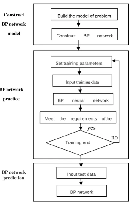
A neural network tool box in MATLAB, first by function, newly achieves the creation of the BP network, this command to create a network object and initialize the network weights and thresholds, the network training function train, network simulation by function seem to achieve the above process can be used to model to solve practical problems, Figure 1 shows the MATLAB using the BP neural network modeling of the flow chart

Network training, pay attention to the choice of the training function (algorithm), the Levenberg-Marquardt algorithm is the fastest algorithm is the first choice to do the simulation. By gradient descent and Newton's method combined with an improved BP method, it has the advantage than the traditional BP and other improvements in the algorithms (such as the four kinds of conjugate gradient method, additional momentum method, adaptive method and quasi-Newton law) convergence speed, network training error is smaller, the function of the MATLAB neural

network simulation tool, LM algorithm is used as default by the BP neural network training function[5], the paper

Fig.1 BP network model to realize flow chart

Instance of verification

Assuming that the evaluation system has 16 evaluations, take the average of each index as input indicators, the actual evaluation of teachers score for the output indicators. Collected a total of 20 teachers in the evaluation of data (Table 1), select the 16-group evaluation of the data used to train the network, the evaluation data used to test the prediction effect. Evaluation Before removing the singular data, neural network has the ability to interpolation, the outer plug a lack of data with more typical and network better generalization ability, 16 groups of teachers in the data must be comprehensive and representative nature, so that the level of achievement with input.

Table 1.Evaluation data of twenty teachers

T1 T2 T3 T4 T5 T6 T7 T8 T9 T10 T11 T12 T13 T14 T15 T16 T17 T18 T19 T20 X1 69.2 86.3 59.0 85.3 91.0 61.0 93.9 80.0 75.3 69.2 93.2 65.2 92.0 88.0 92.0 61.0 72.5 84.0 76.1 89.8 X2 68.0 81.0 58.0 82.0 88.0 61.0 94.4 88.6 75.0 67.5 93.6 66.0 94.0 79.0 85.0 57.4 69.2 79.5 76.0 87.6 X3 69.1 82.8 57.4 84.8 87.8 58.4 93.2 71.9 74.1 72.1 90.8 67.6 94.6 62.6 88.6 57.3 71.6 79.8 74.3 88.7 X4 69.4 85.8 58.7 84.8 90.8 60.7 94.1 75.6 77.4 71.0 92.8 70.4 94.7 84.1 80.6 55.7 73.1 86.8 78.4 86.8 X5 68.1 83.1 56.9 82.1 90.1 58.9 94.3 81.0 74.1 71.1 92.8 63.7 94.5 81.0 81.0 57.9 68.0 82.1 75.1 89.1 X6 68.3 86.3 57.9 81.3 90.9 59.9 93.3 84.3 74.3 63.7 92.7 64.3 94.3 80.0 94.3 55.9 78.4 85.3 75.3 89.4 X7 67.9 85.9 57.3 85.9 89.9 58.3 93.9 76.5 76.9 65.9 91.5 60.4 93.0 85.0 89.0 61.3 69.4 81.9 79.9 87.9 X8 65.3 83.3 58.0 82.8 89.3 60.4 94.1 81.1 77.3 62.8 92.3 68.3 92.0 63.0 93.0 65.0 74.4 81.3 75.3 85.3 X9 69.0 80.7 58.5 81.7 90.9 60.6 93.3 88.0 70.0 71.0 92.2 65.8 92.0 76.0 89.0 58.0 74.5 76.7 74.7 85.7 X10 68.1 83.7 57.4 83.2 91.5 57.4 94.1 80.6 72.1 70.1 92.5 63.7 89.0 72.2 86.0 58.4 67.0 78.7 75.7 86.7 X11 68.4 82.1 57.0 80.1 89.1 58.6 93.9 93.0 71.4 67.4 92.4 63.0 90.0 87.0 93.0 56.5 77.0 80.1 73.1 87.1 X12 67.7 84.7 59.0 79.7 88.7 59.0 93.6 75.6 69.7 62.7 91.9 59.5 91.0 75.0 81.0 59.0 72.0 79.7 72.7 87.7 X13 67.1 81.1 57.4 82.1 89.5 61.4 93.7 87.1 71.1 64.3 92.2 63.0 92.7 81.1 97.1 61.4 73.1 79.6 73.1 86.1 X14 66.0 83.0 58.3 85.0 92.0 59.3 92.7 75.7 71.0 60.5 91.7 60.5 88.7 71.7 79.1 57.3 70.4 80.4 73.0 87.8 X15 67.2 86.2 56.4 83.2 89.3 59.0 93.2 73.4 72.2 65.9 92.6 63.5 92.4 75.4 77.4 60.4 73.8 84.2 78.2 88.2 X16 66.4 84.4 57.0 82.6 88.3 59.9 92.9 79.5 70.4 61.2 91.5 59.5 85.5 77.5 85.5 56.0 68.5 81.4 77.4 86.7 results 67.5 83.9 57.6 82.9 90.0 59.7 93.5 81.5 73.1 66.1 92.3 63.2 91.6 78.5 86.0 58.1 72.2 81.7 75.5 87.8

To the network training data normalized using the maximum minimum value method, normalized corresponding to

the formula as follows:

x

′

=

(

x

−

x

)

/(

x

−

x

)

x

′

x

behalf of the normalized data in a post, xmax =100,xmin=50 on behalf of the categories of indicators in the

maximum and minimum values of the data, pay attention to the scoreless than 50 minutes is not suitable for a

teacher, does not participate in the evaluation of anti-normalization formula is:

Build the model of problem

Construct BP network

BP network Input test data Set training parameters

Input training data

BP neural network

no yes

Meet the requirements ofthe

Training end BP network

practice Construct

BP network

model

min min

max

)

(

x

x

x

x

x

=

′

−

+

Table 2. Evaluation data of twenty teachers by Normalized

T1 T2 T3 T4 T5 T6 T7 T8 T9 T10 T11 T12 T13 T14 T15 T16 T17 T18 T19 T20

X1 0.384 0.726 0.180 0.706 0.820 0.220 0.878 0.600 0.506 0.384 0.864 0.304 0.840 0.760 0.840 0.220 0.450 0.680 0.522 0.796 X2 0.360 0.620 0.160 0.640 0.760 0.220 0.888 0.772 0.500 0.350 0.872 0.320 0.880 0.580 0.700 0.148 0.384 0.590 0.520 0.752 X3 0.382 0.656 0.148 0.696 0.756 0.168 0.864 0.438 0.482 0.442 0.816 0.352 0.892 0.252 0.772 0.146 0.432 0.596 0.486 0.774 X4 0.388 0.716 0.174 0.696 0.816 0.214 0.882 0.512 0.548 0.420 0.856 0.408 0.894 0.682 0.612 0.114 0.462 0.736 0.568 0.736 X5 0.362 0.662 0.138 0.642 0.802 0.178 0.886 0.620 0.482 0.422 0.856 0.274 0.890 0.620 0.620 0.158 0.360 0.642 0.502 0.782 X6 0.366 0.726 0.158 0.626 0.818 0198 0.866 0.686 0.486 0.274 0.854 0.286 0.886 0.600 0.886 0.118 0.568 0.706 0.506 0.788 X7 0.358 0.718 0.146 0.718 0.798 0.166 0.878 0.530 0.538 0.318 0.830 0.208 0.860 0.700 0.780 0.226 0.388 0.638 0.598 0.758 X8 0.306 0.666 0.160 0.656 0.786 0.208 0.882 0.622 0.546 0.256 0.846 0.366 0.840 0.260 0.860 0.300 0.488 0.626 0.506 0.706 X9 0.380 0.614 0.170 0.634 0.818 0.212 0.866 0.760 0.400 0.420 0.844 0.316 0.840 0.520 0.780 0.160 0.490 0.534 0.494 0.714 X10 0.362 0.674 0.148 0.664 0.830 0.148 0.882 0.612 0.442 0.402 0.850 0.274 0.780 0.444 0.720 0.168 0.340 0.574 0.514 0.734 X11 0.368 0.642 0.140 0.602 0.782 0.172 0.878 0.860 0.428 0.348 0.848 0.260 0.800 0.740 0.860 0.130 0.540 0.602 0.462 0.742 X12 0.354 0.694 0.180 0.594 0.774 0.180 0.872 0.512 0.394 0.254 0.838 0.190 0.820 0.500 0.620 0.180 0.440 0.594 0.454 0.754 X13 0.342 0.622 0.148 0.642 0.790 0.228 0.874 0.742 0.422 0.286 0.844 0.260 0.854 0.622 0.942 0.228 0.462 0.592 0.462 0.722 X14 0.320 0.660 0.166 0.700 0.840 0.186 0.854 0.514 0.420 0.210 0.834 0.210 0.774 0.434 0.582 0.146 0.408 0.608 0.460 0.756 X15 0.344 0.724 0.128 0.664 0.786 0.180 0.864 0.468 0.444 0.318 0.852 0.270 0.848 0.508 0.548 0.208 0.476 0.684 0.564 0.764 X16 0.328 0.688 0.140 0.652 0.766 0.198 0.858 0.590 0.408 0.224 0.830 0.190 0.710 0.550 0.710 0.120 0.370 0.628 0.548 0.734 results 0.350 0.678 0.152 0.658 0.800 0.194 0.870 0.630 0.462 0.322 0.846 0.264 0.832 0.570 0.720 0.162 0.444 0.634 0.510 0.756

In this paper, has a hidden layer of BP neural network to evaluate the hidden layer transfer function pure lintansig output layer transfer function. The selected teacher evaluation for the16, the number of neurons of the network input16, the evaluation of the output result is a value, so the number of output neurons of a theoretical research and trial and error, this article selected saphenous nerve and the number7.

The other network parameters need to determine, first of all is the choice of learning rate, learning rate determines the amount of weight change every cycle. Large learning rate may lead to system instability, small learning rate will lead to a longer learning time may be very slow convergence rate, but can guarantee the error value of the network out of the error surface of the trough tends to the minimum error value. Under normal circumstances, tend to select a smaller learning rate in order to ensure the stability of the system. The scope of the learning rate is generally selected between 0.01-0.7, select the learning rate of 0.01, the target error is as small as possible, taking into account the blind pursuit of the training error minimum appears over fitting, to determine the error of1e-5, with 1000 training times and the choice of step10.

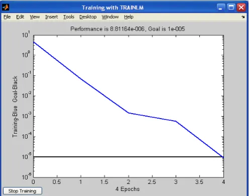
This verification trainlm" algorithm for network training error change graph shown in Figure 2.

Fig 2.The network training error variation pattern (trainlm)

Operation of the network is shown in Figure 3.

Fig 3.The operating results of the network (trainlm)

Table 3. The actual results of the evaluation and the BP network comparative table of the results of the evaluation (“trainlm”)

Results of the evaluation and rating T17 T18 T19 T20 Results of the evaluation of students 72.2 81.7 75.5 87.8 Rating of the evaluation of students middle good middle good Results of the evaluation of nets 72.4 82.3 74.9 88.1 Rating of the evaluation of nets middle good middle good

Network simulation forecast fitting graphics shown in Figure 4.

Fig 4. Network simulation forecast fitting graphics (trainlm)

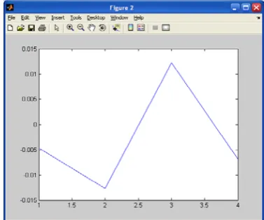
Network simulation prediction error change graphics see figure 5

Fig 5. Network simulation prediction error change graphics (trainlm)

CONCLUSION

we get the following conclusion: in the successful design of BP neural network model based on a reasonable sample of data, neural networks through the training sample, learning to intrinsic regularity of the sample relating to the environment, which can also be input for the future give the correct response, achieving a successful teaching quality assessment.

REFERENCES

[1] CAO Bu-Qing, LIUJian-Xun. Proceedings of the 2010 Second International Conference on Computer Modeling

and Simulation.2010:246-250.

[3]Kitahara M, Achenbach J D, Guo Q C. N. Review of Progress in Quantitative Nondestructive Evaluation, 1992, 11, 701-708.

[4] P. K. Kaiser, Daihua Zou, P. A. Lang. Rock Mechanics and Rock Engineering, 1990, 23(3), 55-59.

[5] Lippmann R P. IEEE Communications Magazine,1989, 27 (11), 47-64.

[6] A Fault Forecasting Model Based On Probabilistic Neural Networks and its Application [A]. Proceedings of the

5th International Symposium on Test and Measurement, 2003, 15-25.

[7] P. K. Kaiser, Daihua Zou, P. A. Lang. Rock Mechanics and Rock Engineering, 1990, 23 (3), 35-45.