On Groebner Bases and Their Use in Solving Some
Practical Problems
Matej Mencinger
1,21University of Maribor, Faculty of Civil Engineering, Smetanova 17, 2000, Maribor, Slovenia 2Institute of Mathematics, Physics and Mechanics, Ljubljana, Jadranska 19, 1000, Ljubljana, Slovenia
*Corresponding Author: [email protected]
Copyright © 2013 Horizon Research Publishing All rights reserved.
Abstract
Groebner basis are an important theoretical building block of modern (polynomial) ring theory. The origin of Groebner basis theory goes back to solving some theoretical problems concerning the ideals in polynomial rings, as well as solving polynomial systems of equations. In this article four practical applications of Groebner basis theory are considered; we use Groebner basis to solve the systems of nonlinear polynomial equations, to solve an integer programming problem, to solve the problem of chromatic number of a graph, and finally we consider an original example from the theory of systems of ordinary (polynomial) differential equations. For practical computations we use systems »MATHEMATICA« and»SINGULAR«.
Keywords
Polynomial system of (differential) equations, integer linear programming, chromatic number of a graph, polynomial rings, Groebner basis, CAS systems1. Introduction
In his 1965 thesis, Bruno Buchberger[3] developed the theory of what we today call Groebner basis. The theory allows computations in multivariate polynomial rings analogous to those we use in single variable polynomial rings. The theory of Groebner basis can also be seen as a generalization of Gaussian elimination of a linear (polynomial) system, which yields the well-known row echelon form. However, applications of Groebner basis can be found in different fields of (mathematical) science. Roughly speaking, they can be used anywhere where some polynomial(s) (ideals) appear.
The basic idea here was to generalize a step in the classical Gaussian elimination algorithm, when for example the pair of polynomials (obtained from equations) 𝑓𝑓 = 3𝑥𝑥 + 7𝑦𝑦 − 5𝑧𝑧 − 2 and 𝑔𝑔 = 2𝑥𝑥 + 3𝑦𝑦 − 8𝑧𝑧 − 6 is replaced by an (equivalent) pair of polynomials (equations)𝑓𝑓 = 3𝑥𝑥 + 7𝑦𝑦 − 5𝑧𝑧 − 2 and𝑆𝑆𝑓𝑓,𝑔𝑔 = 5𝑦𝑦 + 14𝑧𝑧 + 14. Recall that the
least common multiple of 3 and 2 is 6 and that
𝑆𝑆𝑓𝑓,𝑔𝑔 =63(3𝑥𝑥 + 7𝑦𝑦 − 5𝑧𝑧 − 2) −62(2𝑥𝑥 + 3𝑦𝑦 − 8𝑧𝑧 − 6)
= 5𝑦𝑦 + 14𝑧𝑧 + 14. In the sequel we provide some definitions from the ring theory which help to understand the origin of Groebner basis (see e.g. [5] or [13] for details). To this end just recall, that the set of polynomials 𝑓𝑓1, 𝑓𝑓2, … , 𝑓𝑓𝑠𝑠 implies a system of
equations
𝑓𝑓1(𝑥𝑥1, 𝑥𝑥2, … , 𝑥𝑥𝑛𝑛) = 0, 𝑓𝑓2(𝑥𝑥1, 𝑥𝑥2, … , 𝑥𝑥𝑛𝑛)
= 0, … , 𝑓𝑓𝑠𝑠(𝑥𝑥1, 𝑥𝑥2, … , 𝑥𝑥𝑛𝑛) = 0
(1.1)
on one hand, and is naturally associated with the ideal
〈𝑓𝑓1, 𝑓𝑓2, … , 𝑓𝑓𝑠𝑠〉 = �� ℎ𝑗𝑗𝑓𝑓𝑗𝑗: 𝑠𝑠 𝑗𝑗 =1
ℎ1, … , ℎ𝑠𝑠∈ 𝑘𝑘[𝑥𝑥1, 𝑥𝑥2, … , 𝑥𝑥𝑛𝑛]�
generated by polynomials 𝑓𝑓1, 𝑓𝑓2, … , 𝑓𝑓𝑠𝑠 (which is also the
basis of the ideal I = 〈𝑓𝑓1, 𝑓𝑓2, … , 𝑓𝑓𝑠𝑠〉).
The most common monomial term ordering is
lexicographic; though many other are well-known, too (e.g. (graded) reverse lexicographic order, elimination order, etc.).
Recall that as soon as the monomial order is chosen we can speak of leading monomial (LM), leading term(LT) and
leading coefficient (LC) of the polynomial.
Recall also, that any vector 𝑐𝑐⃗ ∈ ℝ𝑛𝑛 defines a weight
(monomial term) ordering <𝑐𝑐⃗ in ℝ[𝑥𝑥1, 𝑥𝑥2, … , 𝑥𝑥𝑛𝑛] in the
following way:
𝑥𝑥𝛼𝛼 <
𝑐𝑐⃗𝑥𝑥𝛽𝛽 ⇔ � 𝑐𝑐⃗ ∙ 𝛼𝛼 < 𝑐𝑐⃗ ∙ 𝛽𝛽𝑐𝑐⃗ ∙ 𝛼𝛼 = 𝑐𝑐⃗ ∙ 𝛽𝛽 𝑎𝑎𝑛𝑛𝑎𝑎 𝛼𝛼 < 𝑜𝑜𝑜𝑜 𝑙𝑙𝑙𝑙𝑥𝑥 𝛽𝛽,
where 𝑐𝑐⃗𝛼𝛼 stands for the standard dot product.
For example, if 𝑐𝑐⃗ = (1,5,10) , we have 𝑥𝑥15𝑥𝑥21𝑥𝑥32<𝑐𝑐⃗𝑥𝑥11𝑥𝑥20𝑥𝑥33 since 𝑐𝑐⃗ ∙ 𝛼𝛼 = (1,5,10) ∙ (5,1,2) = 30
and 𝑐𝑐 ∙����⃗ 𝛽𝛽 = (1,5,10) ∙ (1,0,3) = 31. Note, that for <𝑐𝑐⃗ the
leading term of 𝑔𝑔 = 2𝑥𝑥15𝑥𝑥21𝑥𝑥32− 5𝑥𝑥11𝑥𝑥20𝑥𝑥33 is 𝐿𝐿𝐿𝐿(𝑔𝑔) =
−5𝑥𝑥11𝑥𝑥33 while for <𝑙𝑙𝑙𝑙𝑥𝑥 the leading term of (the same) 𝑔𝑔 is
Once a ring and a monomial order are chosen, one can divide polynomial by another (set of ) polynomial(s). The generalization of the Gaussian elimination process for solving system (1.1) requires to »divide a polynomial by a set of polynomials«. The well-known elementary row operations (from Gaussian elimination) are defined by the fact that on every step 𝑠𝑠 (of the Gaussian elimination process for 𝑓𝑓⃗0(𝑥𝑥⃗) = 0�⃗) the solution of changed system
𝑓𝑓⃗𝑠𝑠(𝑥𝑥⃗) = 0�⃗ remains the same. Let us recall the first example
in context of notation𝑓𝑓⃗𝑠𝑠(𝑥𝑥⃗) = 0�⃗. The initial system:𝑓𝑓0=
3𝑥𝑥 + 7𝑦𝑦 − 5𝑧𝑧 − 2,𝑔𝑔0= 2𝑥𝑥 + 3𝑦𝑦 − 8𝑧𝑧 − 6 is replaced with
𝑓𝑓1= 𝑓𝑓0 , and 𝑔𝑔1= 𝑆𝑆𝑓𝑓,𝑔𝑔= 5𝑦𝑦 + 14𝑧𝑧 + 14 . Note that
𝑔𝑔1= 2𝑓𝑓0− 3𝑔𝑔0+ 0. Note also, that if 𝑓𝑓0(𝑥𝑥�) = 0, 𝑔𝑔0(𝑥𝑥�) =
0 for some 𝑥𝑥�, then 𝑔𝑔1(𝑥𝑥�) = 0, too. The main idea is that
one can replace the initial pair 𝑓𝑓0, 𝑔𝑔0 with 𝑓𝑓1, 𝑔𝑔1 if 𝑓𝑓1 and
𝑔𝑔1 can be »divided between« the initial polynomials, 𝑓𝑓0, 𝑔𝑔0:
𝑓𝑓1= 1𝑓𝑓0+ 0𝑔𝑔0 and 𝑔𝑔1= 2𝑓𝑓0− 3𝑔𝑔0
The division of a polynomial between a set of (other) polynomials is called the multivariable division and lead toward the definition of Groebner bases.
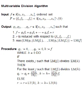
2. The Multivariable Division Algorithm
Considering𝑓𝑓1= 𝑋𝑋𝑋𝑋 − 𝑋𝑋3, 𝑓𝑓2= 𝑋𝑋 + 𝑋𝑋2 and 𝑓𝑓 = 𝑋𝑋2+
𝑋𝑋𝑋𝑋 + 2𝑋𝑋3 and choosing the lexicographic order 𝑋𝑋 > 𝑋𝑋,
then we can easily verify that
𝑓𝑓 = −2𝑓𝑓1+ (𝑋𝑋 + 3𝑋𝑋 − 𝑋𝑋2)𝑓𝑓2+ (−3𝑋𝑋3+ 𝑋𝑋4)
and on the other hand, when the »importance« of 𝑓𝑓1, 𝑓𝑓2 is
chaned to 1. 𝑓𝑓2, 2. 𝑓𝑓1, we have:
𝑓𝑓 = (𝑋𝑋 + 2𝑋𝑋2+ 𝑋𝑋 − 𝑋𝑋2− 2𝑋𝑋𝑋𝑋2+ 2𝑋𝑋4)𝑓𝑓
2+ 0𝑓𝑓1
+ (−3𝑋𝑋3+ 𝑋𝑋4− 2𝑋𝑋6).
Obviously, this multivariable division is very sensitive on the order of 𝑓𝑓1, 𝑓𝑓2 . The order affects the
multi-quotients𝑞𝑞1, 𝑞𝑞2, as well as the remainder𝑜𝑜. When
dividing the polynomial 𝑓𝑓 with the (ordered) set 𝐹𝐹 = (𝑓𝑓1, 𝑓𝑓2) , one can write: 𝑓𝑓 = �{𝑞𝑞1, 𝑞𝑞2}, 𝑜𝑜� instead of
𝑓𝑓 = 𝑞𝑞1𝑓𝑓1+ 𝑞𝑞2𝑓𝑓2+ 𝑜𝑜. Using this notation, in the first case
we have 𝑓𝑓 = �{−2, 𝑋𝑋 + 3𝑋𝑋 − 𝑋𝑋2}, −3𝑋𝑋3+ 𝑋𝑋4� and in the
second case we have 𝑓𝑓 = �{𝑋𝑋 + 2𝑋𝑋2+ 𝑋𝑋 − 𝑋𝑋2− 2𝑋𝑋𝑋𝑋2+
2𝑋𝑋4,0,−3𝑋𝑋3+𝑋𝑋4−2𝑋𝑋6.
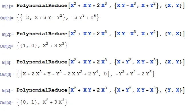
Readily, if one chooses the lexicographic term order 𝑋𝑋 > 𝑋𝑋 the results would be different again, as one can observe from Fig. 1, where system MATHEMATICA is used
[image:2.595.145.476.392.586.2]for the multivariable division. Obviously, 𝑋𝑋 > 𝑋𝑋 gives »simpler« results than 𝑋𝑋 > 𝑋𝑋 (concerning the quotients)
Figure 1. The MATHEMATICA results for multivariable division for different monomial orders. Concerning the problem of multivariable division we have the following result
Theorem 2.1. Fix a monomial order > and let𝐹𝐹 = (𝑓𝑓1, 𝑓𝑓2, … , 𝑓𝑓𝑠𝑠). Then every polynomial𝑓𝑓 ∈ 𝑘𝑘[𝑥𝑥1, 𝑥𝑥2, … , 𝑥𝑥𝑛𝑛] can be
written as
𝑓𝑓 = 𝑞𝑞1𝑓𝑓1+ 𝑞𝑞2𝑓𝑓2+ ⋯ + 𝑞𝑞𝑠𝑠𝑓𝑓𝑠𝑠+ 𝑜𝑜,
where 𝑞𝑞𝑖𝑖, 𝑜𝑜 ∈ 𝑘𝑘[𝑥𝑥1, 𝑥𝑥2, … , 𝑥𝑥𝑛𝑛] and either 𝑜𝑜 = 0 or 𝑜𝑜 is a 𝑘𝑘[𝑥𝑥1, 𝑥𝑥2, … , 𝑥𝑥𝑛𝑛] −linear combination of monomials none of which
are divisible by the leading terms of any of𝑓𝑓1, 𝑓𝑓2, … , 𝑓𝑓𝑠𝑠, which means that 𝑜𝑜 is reduced with respect to 𝐹𝐹 = {𝑓𝑓1, 𝑓𝑓2, … , 𝑓𝑓𝑠𝑠} (i.e.
𝑜𝑜 has lower degree than any ofthe divisors𝑓𝑓1, 𝑓𝑓2, … , 𝑓𝑓𝑠𝑠). We can alternativelly write: 𝑓𝑓⟶ 𝐹𝐹 𝑜𝑜.
Figure 2. Multivariable Division Algorithm.
Recall that the solutions of (1.1) is actually an affine variety
defined by the ideal 𝐼𝐼 = 〈𝑓𝑓1, 𝑓𝑓2, … , 𝑓𝑓𝑠𝑠〉. We would like to use
the division algorithm for the question of ideal membership. If dividing 𝑓𝑓 by 𝑓𝑓1, 𝑓𝑓2, … , 𝑓𝑓𝑠𝑠 gives a remainder of zero then
we know 𝑓𝑓 ∈ 𝐼𝐼. But the converse is not true. Even if 𝑓𝑓 has a nonzero remainder there may be some ways to divide it in a different order that gives a remainder of zero, as we will see in the following example. (Note that the example from Fig.1 shows that the remainders are not unique.)
Let us consider for example 𝑓𝑓1= 𝑥𝑥2− 1, 𝑓𝑓2= 𝑥𝑥𝑦𝑦 + 2
and 𝑓𝑓 = 𝑥𝑥2𝑦𝑦 + 𝑥𝑥𝑦𝑦 + 2𝑥𝑥 + 2 and choose the lexicographic
order 𝑥𝑥 > 𝑦𝑦, then we obtain
𝑓𝑓 = 𝑦𝑦𝑓𝑓1+ 𝑓𝑓2+ (2𝑥𝑥 + 𝑦𝑦).
The remainder 𝑜𝑜 = 2𝑥𝑥 + 𝑦𝑦 ≠ 0, thus one could conclude that 𝑓𝑓 ∉ 〈𝑓𝑓1, 𝑓𝑓2〉, but if the order of divisors is changed to
𝐹𝐹 = (𝑓𝑓2, 𝑓𝑓1), we have 𝑓𝑓⟶ 0 𝐹𝐹; namely
𝑓𝑓 = 0𝑓𝑓1+ (𝑥𝑥 + 1)𝑓𝑓2+ 0 = (𝑥𝑥 + 1)𝑓𝑓2+ 0
and 𝑓𝑓 ∈ 〈𝑓𝑓1, 𝑓𝑓2〉 after all.
Finally, let us consider𝑓𝑓1= 𝑥𝑥 + 𝑦𝑦, 𝑓𝑓2= 𝑥𝑥 − 𝑦𝑦 and
𝑓𝑓 = 2𝑦𝑦 in the ring ℝ[𝑥𝑥, 𝑦𝑦] and fix the lexicographic term order 𝑥𝑥 > 𝑦𝑦. Then obviously 𝑓𝑓 = 𝑓𝑓1− 𝑓𝑓2∈ 〈𝑓𝑓1, 𝑓𝑓2〉, but
since 𝐿𝐿𝐿𝐿(𝑥𝑥 + 𝑦𝑦) = 𝐿𝐿𝐿𝐿(𝑥𝑥 − 𝑦𝑦) = 𝑥𝑥, and because 𝑥𝑥 > 𝑦𝑦 the division algorithm from Fig. 2 returns the remainder 𝑜𝑜 = 2𝑦𝑦. As we shall see, Groebner bases are the solution to the above problems.
3. Groebner Bases
The Groebner basis is a special generating set for our ideals 〈𝑓𝑓1, 𝑓𝑓2, … , 𝑓𝑓𝑛𝑛〉 for which the multivariable division
algorithm for a given 𝑓𝑓 returns the remainder 𝑜𝑜 = 0 if and only if 𝑓𝑓 ∈ 〈𝑔𝑔1, 𝑔𝑔2, … , 𝑔𝑔𝑡𝑡〉.
More precisely, the Groebner basis of an ideal 𝐼𝐼 ⊂ 𝑘𝑘[𝑥𝑥1, 𝑥𝑥2, … , 𝑥𝑥𝑛𝑛] is a finite subset𝐺𝐺 = {𝑔𝑔1, 𝑔𝑔2, … , 𝑔𝑔𝑡𝑡}of 𝐼𝐼
such that
〈𝐿𝐿𝐿𝐿(𝐼𝐼)〉 = 〈𝐿𝐿𝐿𝐿(𝑔𝑔1), 𝐿𝐿𝐿𝐿(𝑔𝑔2), … , 𝐿𝐿𝐿𝐿(𝑔𝑔𝑡𝑡)〉.
Every nonzero ideal 𝐼𝐼 ∈ 𝑘𝑘[𝑥𝑥1, 𝑥𝑥2, … , 𝑥𝑥𝑛𝑛] has the Groebner
basis. Note that 〈𝐿𝐿𝐿𝐿(𝐼𝐼)〉 = 〈𝐿𝐿𝐿𝐿(𝑔𝑔): 𝑔𝑔 ∈ 𝐼𝐼 ∖ {0}〉 = 〈𝐿𝐿𝐿𝐿(𝑔𝑔): 𝑔𝑔 ∈ 𝐼𝐼 ∖ {0}〉 is a monomial ideal and by Dickson's lemma (see [5]) 〈𝐿𝐿𝐿𝐿(𝐼𝐼)〉 =〈𝐿𝐿𝐿𝐿(𝑔𝑔1),𝐿𝐿𝐿𝐿(𝑔𝑔2),…,𝐿𝐿𝐿𝐿(𝑔𝑔𝑡𝑡)〉
=〈LT(𝑔𝑔1),LT(𝑔𝑔2),…,LT(𝑔𝑔𝑡𝑡)〉 for some finite set 𝑔𝑔𝑖𝑖 ∈ 𝐼𝐼.
Furthermore, due to the multivariable division algorithm, if 𝑓𝑓 ∈ 𝐼𝐼 we have 𝑓𝑓 = 𝑞𝑞1𝑔𝑔1+ 𝑞𝑞2𝑔𝑔2+ ⋯ + 𝑞𝑞𝑠𝑠𝑔𝑔𝑠𝑠+ 𝑜𝑜 and no
term of 𝑜𝑜 is divisible by any of 𝐿𝐿𝐿𝐿(𝑔𝑔1), 𝐿𝐿𝐿𝐿(𝑔𝑔2), … , 𝐿𝐿𝐿𝐿(𝑔𝑔𝑡𝑡).
Thus,
𝑜𝑜 = 𝑓𝑓 − (𝑞𝑞1𝑔𝑔1+ 𝑞𝑞2𝑔𝑔2+ ⋯ + 𝑞𝑞𝑠𝑠.
so 𝐿𝐿𝐿𝐿(𝑜𝑜) ∈ 〈𝐿𝐿𝐿𝐿(𝐼𝐼)〉 = 〈𝐿𝐿𝐿𝐿(𝑔𝑔1), 𝐿𝐿𝐿𝐿(𝑔𝑔2), … , 𝐿𝐿𝐿𝐿(𝑔𝑔𝑡𝑡)〉. But no
term of 𝑜𝑜 is divisible by any of the 𝐿𝐿𝐿𝐿(𝑔𝑔𝑖𝑖) and so we must
have 𝑜𝑜 = 0, which implies:
𝑓𝑓 ∈ 〈𝐿𝐿𝐿𝐿(𝑔𝑔1), 𝐿𝐿𝐿𝐿(𝑔𝑔2), … , 𝐿𝐿𝐿𝐿(𝑔𝑔𝑡𝑡)〉.
Obviously, if 𝐺𝐺 = {𝑔𝑔1, 𝑔𝑔2, … , 𝑔𝑔𝑡𝑡} is the Groebner basis
of 𝐼𝐼, the remainder of any 𝑓𝑓 ∈ 𝐼𝐼(after applying the multidivision algorithm) is unique. If 𝑓𝑓 = 𝑞𝑞1𝑔𝑔1+ 𝑞𝑞2𝑔𝑔2+
⋯ + 𝑞𝑞𝑠𝑠𝑔𝑔𝑠𝑠+ 𝑜𝑜 and 𝑓𝑓 = 𝑞𝑞1′𝑔𝑔1+ 𝑞𝑞2′𝑔𝑔2+ ⋯ + 𝑞𝑞𝑠𝑠′𝑔𝑔𝑠𝑠+ 𝑜𝑜′
then 𝑜𝑜 − 𝑜𝑜′ = (𝑞𝑞
1− 𝑞𝑞1′)𝑔𝑔1+ ⋯ + (𝑞𝑞𝑠𝑠− 𝑞𝑞𝑠𝑠′)𝑔𝑔𝑠𝑠∈ 𝐼𝐼 . If
𝑜𝑜 − 𝑜𝑜′ ≠ 0 then 𝐿𝐿𝐿𝐿(𝑜𝑜 − 𝑜𝑜′) ∈ 〈𝐿𝐿𝐿𝐿(𝐼𝐼)〉which implies that
𝐿𝐿𝐿𝐿(𝑔𝑔𝑖𝑖) divides 𝐿𝐿𝐿𝐿(𝑜𝑜 − 𝑜𝑜′) for some 𝑖𝑖. But this leads to a
contradiction, since no term of 𝑜𝑜 or 𝑜𝑜′ is divisible by any 𝐿𝐿𝐿𝐿(𝑔𝑔𝑖𝑖). Thus, we must have 𝑜𝑜 = 𝑜𝑜′ and therefore 𝑔𝑔 = 𝑔𝑔′.
Testing whether a basis is a Groebner basis is intimately connected with the so called 𝑆𝑆 −polynomial for a given pair of polynomials 𝑓𝑓, 𝑔𝑔 ∈ 𝑘𝑘[𝑥𝑥1, 𝑥𝑥2, … , 𝑥𝑥𝑛𝑛]; a generalization of
𝑆𝑆𝑓𝑓,𝑔𝑔− polynomial defined in the introduction. The
𝑆𝑆 −polynomial of 𝑓𝑓 and 𝑔𝑔 is defined as follows. Let 𝑓𝑓, 𝑔𝑔 ∈ 𝑘𝑘[𝑥𝑥1, 𝑥𝑥2, … , 𝑥𝑥𝑛𝑛]be nonzero polynomials. Find the
least common multiple of their leading monomials:𝑥𝑥𝛾𝛾 =
𝐿𝐿𝐿𝐿𝐿𝐿(𝐿𝐿𝐿𝐿(𝑓𝑓), 𝐿𝐿𝐿𝐿(𝑔𝑔)). Then the 𝑆𝑆 −polynomial of 𝑓𝑓 and 𝑔𝑔 is defined by:
𝑆𝑆(𝑓𝑓, 𝑔𝑔) =𝐿𝐿𝐿𝐿(𝑓𝑓) ⋅ 𝑓𝑓 −𝑥𝑥𝛾𝛾 𝐿𝐿𝐿𝐿(𝑔𝑔) ⋅ 𝑔𝑔.𝑥𝑥𝛾𝛾
Note, that the 𝑆𝑆 −polynomials provide cancellacion of leading terms and in fact are the only way that cancelation happens among sums of terms of the same multi-degree.
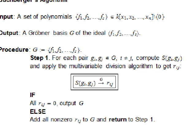
The Buchcberger's basic observation was the following
criterion. Let 𝐼𝐼 be an ideal. Then 𝐺𝐺 = {𝑔𝑔1, 𝑔𝑔2, … , 𝑔𝑔𝑡𝑡} is a
Groebner bases (for 𝐼𝐼) if and only if for all 𝑖𝑖 ≠ 𝑗𝑗 the remainder on division of 𝑆𝑆(𝑔𝑔𝑖𝑖, 𝑔𝑔𝑗𝑗) by 𝐺𝐺 is zero:
𝑆𝑆(𝑔𝑔𝑖𝑖 , 𝑔𝑔𝑗𝑗)⟶ 𝐺𝐺 0 ∀𝑖𝑖≠𝑗𝑗 .
This criterion is the basis of the famous Buchberger's algorithm, which produces the Groebner bases for the nonzero ideal 𝐼𝐼 = 〈𝑓𝑓1, 𝑓𝑓2, … , 𝑓𝑓𝑠𝑠〉. The Buchberger's algorithm
[image:4.595.157.469.310.516.2]is shown in Fig. 3 [13].
Figure 3. Buchberger's Algorithm: returns a Groebner basis of 𝐼𝐼 = 〈𝑓𝑓1, 𝑓𝑓2, … , 𝑓𝑓𝑛𝑛〉.
Note, that the most efficient computer algebra systems have routines to produce Groebner bases. An example in
MATHEMATICA is shown in Fig. 4. Since the Buchberger’s Algorithm is based on the Multivariable Division Algorithm,
which depends on the monomial term order, the computing of Groebner basis will depend on the monomial term order, as well. In Fig.4 in »In[1]:=« we want to compute the Groebner basis with respect to the lexicographic term order with 𝑥𝑥 > 𝑦𝑦, whilst in »In[2]:=« with respect to the lexicographic term order with 𝑦𝑦 > 𝑥𝑥.
Note, that Buchberger's algorithm produces a lot of »extra« basis elements than needed (i.e. it is not optimal). If we require an extra condition that no term of 𝑔𝑔𝑖𝑖 is divisible by any 𝐿𝐿𝐿𝐿(𝑔𝑔𝑗𝑗) and in order to ensure the uniqueness of 𝐺𝐺 (provided the
monomial term order is fixed) we also require that each 𝑔𝑔𝑖𝑖 is monic (i.e.𝐿𝐿𝐿𝐿(𝑔𝑔𝑖𝑖) = 1 for all 𝑖𝑖 = 1,2, … , 𝑡𝑡), then we get the so
called reduced Groebner basis. The reduced Groebner basis always exists and is unique (see e.g. [13] for the proof). The simple algorithm which produces the reduced Groebner basis beginning with any Groebner basis 𝐺𝐺 is the following: begin with 𝐺𝐺 and make all 𝑔𝑔𝑖𝑖 ∈ 𝐺𝐺 monic, for any 𝑔𝑔 ∈ 𝐺𝐺, replace 𝑔𝑔 by its remainder upon division of 𝑔𝑔 by elements if 𝐺𝐺 ∖ {𝑔𝑔}
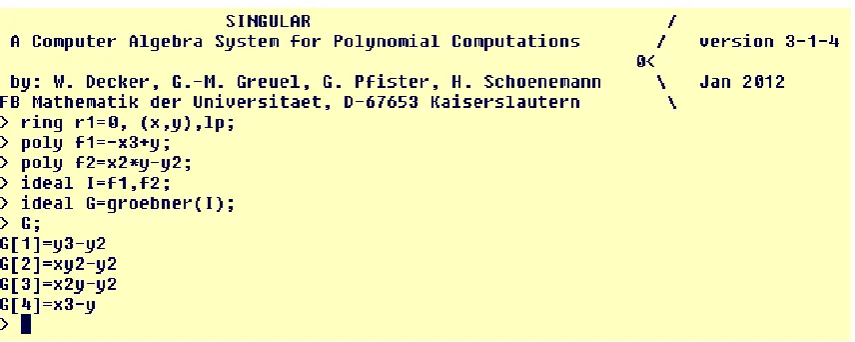
(in the fixed monomial term order). Of course, the routines in all computer algebra systems already return the reduced Groebner basis. In Fig. 5 and 6 Groebner basis of {−𝑥𝑥3+ 𝑦𝑦, 𝑥𝑥2𝑦𝑦 − 𝑦𝑦2} in the lexicographic term order are computed in
system MATHEMATICA and SINGULAR. We see that MATHEMATICA returns {−𝑦𝑦2+ 𝑦𝑦3, −𝑦𝑦2+ 𝑥𝑥𝑦𝑦2, 𝑥𝑥2𝑦𝑦 − 𝑦𝑦2, 𝑥𝑥3− 𝑦𝑦},
[image:5.595.93.521.272.443.2]while SINGULAR returns 𝐺𝐺[1] = 𝑦𝑦3 − 𝑦𝑦2, 𝐺𝐺[2] = 𝑥𝑥𝑦𝑦2 − 𝑦𝑦2, 𝐺𝐺[3] = 𝑥𝑥2𝑦𝑦 − 𝑦𝑦2, 𝐺𝐺[4] = 𝑥𝑥3 − 𝑦𝑦.
Figure 5. Output of Groebner bases in system MATHEMATICA
Figure 6. Output of Groebner bases in system SINGULAR
One reason to turn to more special systems than MATHEMATICA is to compute the Groebner basis in a special monomial
term order or simply to reduce a polynomial (in sense of the multivariable division algorithm) in a special monomial term order. In Fig. 7 we show the Groebner basis of {−𝑥𝑥3+ 𝑦𝑦, 𝑥𝑥2𝑦𝑦 − 𝑦𝑦2} computed in SINGULAR with respect to the weight order
[image:5.595.83.526.540.701.2]with weight vector (1,3). Note, that the result 𝐺𝐺<(1,3)= {𝑥𝑥3− 𝑦𝑦, 𝑦𝑦2− 𝑥𝑥2𝑦𝑦} is not the same as the Groebner basis computed in the lexicographic monomial order 𝐺𝐺<𝑙𝑙𝑙𝑙𝑥𝑥 (𝑦𝑦>𝑥𝑥)= {−𝑥𝑥5+ 𝑥𝑥6, −𝑥𝑥3+ 𝑦𝑦}.
Figure 7. Groebner basis𝐺𝐺<(1,3) of {𝑥𝑥3− 𝑦𝑦, −𝑥𝑥2𝑦𝑦 + 𝑦𝑦2} computed in SINGULAR
As mentioned before, we seek solutions (𝑎𝑎1, 𝑎𝑎2, … , 𝑎𝑎𝑛𝑛) ∈ 𝑘𝑘� of polynomial system
𝑓𝑓1(𝑥𝑥1, 𝑥𝑥2, … , 𝑥𝑥𝑛𝑛) = 0, 𝑓𝑓2(𝑥𝑥1, 𝑥𝑥2, … , 𝑥𝑥𝑛𝑛) = 0, … , 𝑓𝑓𝑠𝑠(𝑥𝑥1, 𝑥𝑥2, … , 𝑥𝑥𝑛𝑛) = 0, (4.1)
where 𝑘𝑘� is the algebraic closure of 𝑘𝑘[𝑥𝑥1, 𝑥𝑥2, … , 𝑥𝑥𝑛𝑛]. The following theorem gives a criterion on existence of solutions of
(4.1). For a proof, see [1]. Let 𝐺𝐺 = {𝑔𝑔1, 𝑔𝑔2, … , 𝑔𝑔𝑡𝑡} be the reduced Groebner basis of 〈𝑓𝑓1, 𝑓𝑓2, … , 𝑓𝑓𝑠𝑠〉. There are no solutions to
the system (4.1) if and only if 𝐺𝐺 = {1}. If (4.1) has finitely many solutions, we say that 〈𝑓𝑓1, 𝑓𝑓2, … , 𝑓𝑓𝑠𝑠〉 is zero-dimensional.
Concerning Groebner basis, 〈𝑓𝑓1, 𝑓𝑓2, … , 𝑓𝑓𝑠𝑠〉 (corresponding to (4.1)) is zero-dimensional if and only if for every 𝑖𝑖 = 1,2, … , 𝑛𝑛,
there exists 𝑗𝑗 ∈ {1,2, … , 𝑡𝑡} such that 𝐿𝐿𝐿𝐿(𝑔𝑔𝑖𝑖) = 𝑥𝑥𝑖𝑖𝛼𝛼 for some 𝛼𝛼 ∈ ℕ0𝑛𝑛 . Note, that if 𝐼𝐼 = 〈𝑓𝑓1, 𝑓𝑓2, … , 𝑓𝑓𝑠𝑠〉 is not
zero-dimensional, one has to compute the so called primary decomposition of 𝐼𝐼, which is much more complicated then the computations presented in the following example; see [13] for more details.
We want to solve the example from [6]:
𝑓𝑓1 = 𝑥𝑥2+ 𝑦𝑦𝑧𝑧 + 𝑥𝑥 = 0, 𝑓𝑓2 = 𝑧𝑧2+ 𝑥𝑥𝑦𝑦 + 𝑧𝑧 = 0, 𝑓𝑓3 = 𝑦𝑦2+ 𝑥𝑥𝑧𝑧 + 𝑦𝑦 = 0. (4.2)
To that end, fix the term order to be lexicographic 𝑥𝑥 > 𝑦𝑦 > 𝑧𝑧. We find Groebner basis of 〈𝑓𝑓1, 𝑓𝑓2, 𝑓𝑓3〉 using system
MATHEMATICA (see Fig. 8):
Figure 8. Groebner basis of 〈𝑓𝑓1, 𝑓𝑓2, 𝑓𝑓3〉 associated to (4.1). Since the first polynomial depends only on 𝑧𝑧, 𝑧𝑧 is either 0,
−12 or −1. The system has obviously finitely many solutions, since the third polynomial in 𝐺𝐺 contains only 𝑧𝑧 and 𝑦𝑦 and its leading power product is 𝑦𝑦2. And finally, the
last polynomial contains 𝑥𝑥and𝑦𝑦and 𝑧𝑧and its leading power product is 𝑥𝑥2. If 𝑧𝑧 = 0 the system becomes 𝑦𝑦 + 𝑦𝑦2=
0, 𝑥𝑥𝑦𝑦 = 0, 𝑥𝑥 + 𝑥𝑥2= 0. And the (reduced) set of polynomials
is already a reduced Groebner basis of the ideal it generates. The corresponding solutions are 𝑦𝑦 = 0 and 𝑥𝑥 = 0 or 𝑥𝑥 = −1 and 𝑦𝑦 = −1and 𝑥𝑥 = 0. Our solutions so far are (0,0,0), (−1,0,0) and (0, −1,0). Similar, for 𝑧𝑧 = −1 we get 𝑦𝑦2= 0, −𝑥𝑥 + 𝑦𝑦 = 0, 𝑥𝑥𝑦𝑦 = 0, 𝑥𝑥 + 𝑥𝑥2− 𝑦𝑦 = 0 . The
corresponding reduced Groebner basis is {𝑦𝑦, 𝑥𝑥}, which yields 𝑥𝑥 = 𝑦𝑦 = 0. So another solution is (0,0, −1). Similar we get for 𝑧𝑧 = −12 the corresponding reduced Groebner basis:{2𝑦𝑦 + 1,2𝑥𝑥 + 1}, which yields the final solution (−12, −12, −12).
5. Groebner Bases and Integer Linear
Programming
Let 𝑎𝑎𝑖𝑖,𝑗𝑗 ∈ ℤ, 𝑏𝑏𝑖𝑖 ∈ ℤ and 𝑐𝑐𝑗𝑗 ∈ ℝ with 𝑖𝑖 = 1,2, … , 𝑛𝑛 and
𝑗𝑗 = 1,2, … , 𝑚𝑚. We seek a solution 𝑥𝑥⃗ = (𝑥𝑥1, 𝑥𝑥2, … , 𝑥𝑥𝑛𝑛) of the
system
𝑎𝑎11𝑥𝑥1+ 𝑎𝑎12𝑥𝑥2+ ⋯ + 𝑎𝑎1𝑛𝑛𝑥𝑥𝑛𝑛 = 𝑏𝑏1
⋮
𝑎𝑎𝑚𝑚1𝑥𝑥1+ 𝑎𝑎𝑚𝑚2𝑥𝑥2+ ⋯ + 𝑎𝑎𝑚𝑚𝑛𝑛𝑥𝑥𝑛𝑛 = 𝑏𝑏𝑚𝑚 ,
(5.1)
which minimizes the cost function 𝑐𝑐(𝑥𝑥1, 𝑥𝑥2, … , 𝑥𝑥𝑚𝑚) =
∑𝑛𝑛𝑗𝑗 =1𝑐𝑐𝑗𝑗𝑥𝑥𝑗𝑗. We call (5.1) an integer (linear) program (IP) and
write it in a matrix form:
minimize 𝑐𝑐⃗ ∙ 𝑥𝑥⃗ subject to 𝐴𝐴𝑥𝑥⃗ = 𝑏𝑏�⃗, where 𝐴𝐴 ∈ ℤ𝑚𝑚×𝑛𝑛 and 𝑏𝑏�⃗ = (𝑏𝑏
1, … , 𝑏𝑏𝑚𝑚) ∈ ℤ𝑚𝑚.
We will consider just the main mathematical idea which makes use of Groebner bases when solving IP (5.1). We can associate to (5.1) new variables 𝑋𝑋𝑘𝑘; 𝑘𝑘 = 1,2, … , 𝑚𝑚 to
represent the 𝑘𝑘 −th equation in (5.1) as: 𝑋𝑋𝑘𝑘𝑎𝑎𝑘𝑘1𝑥𝑥1+𝑎𝑎𝑘𝑘2𝑥𝑥2+⋯+𝑎𝑎𝑘𝑘𝑛𝑛𝑥𝑥𝑛𝑛 = 𝑋𝑋
𝑘𝑘𝑏𝑏𝑘𝑘.
Of course, we can then write the whole system as 𝑋𝑋1𝑎𝑎11𝑥𝑥1+𝑎𝑎12𝑥𝑥2+⋯+𝑎𝑎1𝑛𝑛𝑥𝑥𝑛𝑛⋯ 𝑋𝑋
𝑚𝑚𝑎𝑎𝑚𝑚 1𝑥𝑥1+𝑎𝑎𝑚𝑚 2𝑥𝑥2+⋯+𝑎𝑎𝑚𝑚𝑛𝑛𝑥𝑥𝑛𝑛
= 𝑋𝑋1𝑏𝑏1⋯ 𝑋𝑋
𝑚𝑚𝑏𝑏𝑚𝑚,
which is equivalent to �𝑋𝑋1𝑎𝑎11⋯ 𝑋𝑋
𝑚𝑚𝑎𝑎𝑚𝑚 1�𝑥𝑥1∙ ⋯ ∙ �𝑋𝑋1𝑎𝑎1𝑛𝑛⋯ 𝑋𝑋𝑚𝑚𝑎𝑎𝑚𝑚𝑛𝑛�𝑥𝑥𝑛𝑛 = 𝑋𝑋⃗𝑏𝑏�⃗.
Next, to each column of (5.1) or equivalently to each term in the brackets (… ) in the above equation we associate a new variable 𝑋𝑋𝑘𝑘 = 𝑋𝑋1𝑎𝑎1𝑘𝑘⋯ 𝑋𝑋𝑚𝑚𝑎𝑎𝑚𝑚𝑘𝑘; for each 𝑘𝑘 = 1,2, … , 𝑛𝑛. The
first step in solving our problem is to figure out whether a solution exists at all. The theory of Groebner bases helps to characterize the existence and optimality of IP (5.1). The main idea is connected with the following ring homomorphism Φ: 𝑘𝑘[𝑋𝑋1, … , 𝑋𝑋𝑛𝑛] → 𝑘𝑘[𝑋𝑋1, … , 𝑋𝑋𝑚𝑚], defined by:
yielding Φ(𝑋𝑋1𝑥𝑥1⋅ ⋯ ∙ 𝑋𝑋𝑛𝑛𝑥𝑥𝑛𝑛) = 𝑋𝑋⃗𝑏𝑏�⃗. This implies (see [9] for
details) the following: there exist a solution to IP (5.1) (i.e. a vector 𝑥𝑥⃗ = 𝑥𝑥� such that 𝐴𝐴𝑥𝑥� = 𝑏𝑏�⃗) if and only if 𝑋𝑋⃗𝑏𝑏�⃗ is in the
image of Φ; yielding ∃𝑃𝑃 such that 𝑃𝑃 = 𝑋𝑋�⃗𝑥𝑥� for some
𝑥𝑥� ∈ ℕ0𝑛𝑛.
Next, the basic idea of Conti & Traverso's algorithm[4] is presented. But first we have to consider how to transform (5.1) which can contain some negative integres; recall that 𝑎𝑎𝑖𝑖,𝑗𝑗 ∈ ℤ and 𝑏𝑏𝑖𝑖 ∈ ℤ. This can be generally transformed to an
IP with strictly nonnegative (integer) coefficients 𝑎𝑎𝑖𝑖,𝑗𝑗, 𝑏𝑏𝑖𝑖 by
adding an extra indeterminate 𝑊𝑊defined by
𝑋𝑋1∙ 𝑋𝑋2∙ ⋯ ∙ 𝑋𝑋𝑚𝑚∙ 𝑊𝑊 = 1, (5.3)
which transforms 𝑋𝑋1𝑎𝑎1𝑗𝑗 ∙ ⋯ ∙ 𝑋𝑋
𝑖𝑖
−𝑎𝑎𝑖𝑖𝑗𝑗 ∙ ⋯ ∙ 𝑋𝑋
𝑚𝑚𝑎𝑎𝑚𝑚𝑗𝑗 to
𝑋𝑋1𝑎𝑎1𝑗𝑗+𝑎𝑎𝑖𝑖𝑗𝑗 ⋯ ∙ 𝑋𝑋
𝑖𝑖0∙ ⋯ ∙ 𝑋𝑋𝑚𝑚𝑎𝑎𝑚𝑚𝑗𝑗+𝑎𝑎𝑖𝑖𝑗𝑗 ∙ 𝑊𝑊𝑎𝑎𝑖𝑖𝑗𝑗 =: 𝑋𝑋⃗𝐴𝐴𝑗𝑗𝑊𝑊𝑗𝑗.
If there are some negative entries in 𝑏𝑏�⃗, we transform 𝑋𝑋⃗𝑏𝑏�⃗ to
𝑋𝑋⃗𝑏𝑏�⃗𝑊𝑊
𝑏𝑏�⃗ in a similar way.
The optimal solution of IP (5.1) with some negative integers is therefore obtained in the following way:
• Define 𝑊𝑊 by (5.3), if there are some negative entries in 𝐴𝐴, 𝑏𝑏�⃗
• Define an ideal 𝐼𝐼 = �𝑋𝑋1− 𝑋𝑋⃗𝐴𝐴1, … , 𝑋𝑋𝑛𝑛− 𝑋𝑋⃗𝐴𝐴𝑛𝑛� on the
polynomial ring 𝑘𝑘[𝑋𝑋1, … , 𝑋𝑋𝑚𝑚, 𝑋𝑋1, … , 𝑋𝑋𝑛𝑛], if there are no
negative entries in 𝐴𝐴, 𝑏𝑏�⃗
• Define an ideal 𝐼𝐼 = �𝑋𝑋1− 𝑋𝑋⃗𝐴𝐴1𝑊𝑊1, … , 𝑋𝑋𝑛𝑛− 𝑋𝑋⃗𝐴𝐴𝑛𝑛𝑊𝑊𝑛𝑛, 𝑋𝑋1∙
𝑋𝑋2∙⋯∙𝑋𝑋𝑚𝑚∙𝑊𝑊−1 on the polynomial ring 𝑘𝑘[𝑋𝑋1, … , 𝑋𝑋𝑚𝑚, 𝑊𝑊, 𝑋𝑋1, … , 𝑋𝑋𝑛𝑛], if there are some negative entries
in 𝐴𝐴, 𝑏𝑏�⃗
• Let 𝐺𝐺 be the reduced Groebner basis of 𝐼𝐼with respect to a monomial order <𝑐𝑐⃗, where 𝑐𝑐⃗ is defined by the cost
function 𝑐𝑐⃗ ∙ 𝑥𝑥⃗
• Dividing 𝑋𝑋⃗𝑏𝑏�⃗𝑊𝑊
𝑏𝑏�⃗(i.e. the generalization of 𝑋𝑋⃗𝑏𝑏�⃗) by
𝐺𝐺always yields a remainder 𝑅𝑅 ∈ 𝑘𝑘[𝑋𝑋1, … , 𝑋𝑋𝑛𝑛], which ensures
the optimality of the solution due to its minimality (ensured by the multivariable division algorithm); thus the solution 𝑥𝑥⃗ = (𝛽𝛽1, … , 𝛽𝛽𝑛𝑛) to IP (5.1) is obtained by reducing 𝑋𝑋⃗𝑏𝑏�⃗𝑊𝑊𝑏𝑏�⃗
by 𝐺𝐺 which yields a remainder 𝑅𝑅 = 𝑋𝑋1𝛽𝛽1⋯ 𝑋𝑋𝑛𝑛𝛽𝛽𝑛𝑛 and
thereby the solution 𝑥𝑥⃗ = (𝛽𝛽1, … , 𝛽𝛽𝑛𝑛).
Next, we consider the example from [9]. Following (5.1), we have to minimize the cost function
𝑐𝑐⃗ ∙ 𝑥𝑥⃗ = 1000𝑥𝑥1+ 𝑥𝑥2+ 𝑥𝑥3+ 100𝑥𝑥4
subject to
3𝑥𝑥1− 2𝑥𝑥2+ 𝑥𝑥3− 𝑥𝑥4= −1
4𝑥𝑥1+ 𝑥𝑥2− 𝑥𝑥3 = 5. (5.4)
The solution to the above example obtained with system
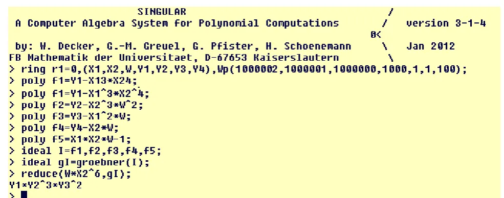
SINGULAR is shown in Fig.9. The weighted term order is used
with 𝐿𝐿⃗ = ( 1000002,1000001,1000000,1000,1,1,100) to ensure that 𝑋𝑋1 > 𝑋𝑋2 > 𝑊𝑊 > 𝑋𝑋1 > 𝑋𝑋2 > 𝑋𝑋3 > 𝑋𝑋4 and to ensure the weight order (1000,1,1,100), corresponding to 𝑐𝑐⃗ = (1000,1,1,100) . Note, that for example the monomials 𝑋𝑋⃗𝑏𝑏�⃗𝑊𝑊
𝑏𝑏�⃗ and 𝑋𝑋⃗𝐴𝐴2𝑊𝑊2 are:
𝑋𝑋⃗𝑏𝑏�⃗𝑊𝑊
𝑏𝑏�⃗= 𝑋𝑋1−1𝑋𝑋25= 𝑋𝑋1−1𝑋𝑋2−1∙ 𝑋𝑋21𝑋𝑋25= 𝑊𝑊1𝑋𝑋26,
𝑋𝑋⃗𝐴𝐴2𝑊𝑊
2= 𝑋𝑋1−2𝑋𝑋21= 𝑋𝑋1−2𝑋𝑋2−2∙ 𝑋𝑋22𝑋𝑋21= 𝑊𝑊2𝑋𝑋23.
The optimal solution 𝑥𝑥⃗ = (1,3,2,0) is obtained from the result of the multivariable division:
[image:7.595.57.550.474.668.2]𝑊𝑊1𝑋𝑋26⟶ 𝐺𝐺 𝑋𝑋11𝑋𝑋23𝑋𝑋32𝑋𝑋4.0
6. Groebner Bases and Computing the
Chromatic Number
One of the most important and applied things in graph theory is the chromatic number of a graph. It is defined as the smallest number of colours needed to colour the vertices of graph 𝐺𝐺 = (𝑉𝑉, 𝐸𝐸) so that no two adjacent vertices 𝑘𝑘, 𝑠𝑠 ∈ 𝑉𝑉 share the same colour. For many (families) of graphs the chromatic numbers are known (i.e. defined in terms of the number of its vertices and/or edges). Probably the most simple examples are cycle graphs 𝐿𝐿𝑛𝑛: a cycle
graph 𝐿𝐿2𝑘𝑘 has chromatic number 2, whilst 𝐿𝐿2𝑘𝑘+1 has
chromatic number 3, which is usually denoted by 𝒳𝒳(𝐿𝐿2𝑘𝑘+1) = 3, 𝒳𝒳(𝐿𝐿2𝑘𝑘) = 2. There are many well-known
conjectures and open problems concerning the chromatic number of (undirected) graphs (e.g. Hadwiger conjecture, Albertson conjecture, Erdös–Faber–Lovász conjecture). The subject inspired many researchers (e.g. [2,11,15]). The idea of finding a 𝑛𝑛 −colloring and consequently the chromatic number of a given graph using Groebner bases is to associate a variable 𝑥𝑥[𝑘𝑘] to each vertex 𝑘𝑘 of the graph and to reduce the problem to the solution of a system of polynomial equations. The 𝑛𝑛 −th roots of unity is used as 𝑛𝑛 colours. Since variables 𝑥𝑥[𝑘𝑘] represent the vertices, the condition that a vertex 𝑘𝑘 should have a colour is then associated to roots of
𝑥𝑥[𝑘𝑘]𝑛𝑛− 1 = 0 (6.1)
and the polynomial (𝑥𝑥[𝑘𝑘]𝑛𝑛− 𝑥𝑥[𝑠𝑠]𝑛𝑛)/(𝑥𝑥[𝑘𝑘] − 𝑥𝑥[𝑠𝑠] ) is
associated to the condition that the vertices 𝑘𝑘 and 𝑠𝑠 (corresponding to 𝑥𝑥[𝑘𝑘] and 𝑥𝑥[𝑠𝑠]) must have different colours (see also [1]). Thus, if vertices 𝑘𝑘 and 𝑠𝑠 are adjacent and the graph has to be coloured by 𝑛𝑛 colours, the polynomial
𝐹𝐹𝑛𝑛[𝑘𝑘, 𝑠𝑠] = 𝑥𝑥[𝑘𝑘]𝑛𝑛−1+ 𝑥𝑥[𝑘𝑘]𝑛𝑛−2𝑥𝑥[𝑠𝑠]1+ ⋯
+ 𝑥𝑥[𝑘𝑘]1𝑥𝑥[𝑠𝑠]𝑛𝑛−2+ 𝑥𝑥[𝑠𝑠]𝑛𝑛−1 (6.2)
must vanish. Thus finding a chromatic number of a given graph 𝐺𝐺 = (𝑉𝑉, 𝐸𝐸) with |𝑉𝑉| = 𝑁𝑁 is then obtained by
applying the following algorithm:
• Input: Graph 𝐺𝐺 = (𝑉𝑉, 𝐸𝐸) (i.e. vertices 𝑥𝑥[1], … , 𝑥𝑥[𝑁𝑁] and the adjacency matrix 𝐴𝐴(𝐺𝐺))
• Output: chromatic number 𝒳𝒳(𝐺𝐺)
• Procedure:
• 𝑛𝑛 ≔ 1
• WHILE 𝐺𝐺𝐼𝐼𝑛𝑛 = {1} DO 𝐼𝐼 =∪𝑘𝑘=1𝑁𝑁 {𝑥𝑥[𝑘𝑘]𝑛𝑛− 1}
• For all adjacent vertices 𝑘𝑘 and 𝑠𝑠 compute polynomial 𝐹𝐹𝑛𝑛[𝑘𝑘, 𝑠𝑠] defined by (6.2) and add it to the ideal 𝐼𝐼:
𝐼𝐼: = 𝐼𝐼 ∪ 𝐹𝐹𝑛𝑛[𝑘𝑘, 𝑠𝑠]
• Compute Groebner basis 𝐺𝐺𝐼𝐼𝑛𝑛 of 𝐼𝐼
• IF 𝐺𝐺𝐼𝐼𝑛𝑛 = {1} THEN 𝑛𝑛 ≔ 𝑛𝑛 + 1
• Find a solution (i.e. colouring) of 𝐺𝐺𝐼𝐼𝑛𝑛 = {0, … ,0}; 𝒳𝒳(𝐺𝐺) = 𝑛𝑛
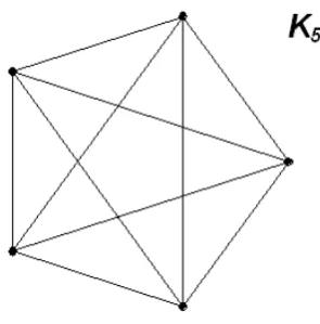
As an example, the computation of 𝒳𝒳(G) (where 𝐺𝐺 = 𝐾𝐾5 -
a complete graph on 5 vertices; see Fig. 10) using the basic system MATHEMATICA is presented in Figs. 11 and 12. In Fig.
11 we see that 𝐺𝐺𝐼𝐼3 = {1}. Similarly we obtain that 𝐺𝐺𝐼𝐼4 = {1}. Note that the command
Do[Print[Fn[𝑘𝑘, 𝑠𝑠]], {𝑘𝑘, 𝑁𝑁}, {𝑠𝑠, 𝑘𝑘 − 1}]
[image:8.595.357.505.385.535.2]is very useful since it gives a list of all possible edges.
Figure 10. Graph 𝐺𝐺 = 𝐾𝐾5.
Figure 12. Computing 𝐺𝐺𝐼𝐼5 for 𝐺𝐺 = 𝐾𝐾5; 𝑛𝑛 = 5 and solving system »GI5=0«.
In Fig. 12 GI5 is computed and the solution to GI5 = 0 is verified. Though it is well-known that 𝒳𝒳(𝐾𝐾𝑛𝑛) = 𝑛𝑛, yet
the example is very practical and instructive (since 𝐾𝐾𝑛𝑛
contains all (simple) edges on 𝑛𝑛 points). In package »Combinatorica« it is possible to compute the chromatic number of a given graph in MATHEMATICA. However, the
above procedure may be useful to handle some general (families of) graphs.
7. Groebner Bases and Systems of
ODE‘s
Concerning the qualitative analysis of systems of ODE's (e.g. solving the center-focus problem, cyclicity problems, critical period perturbations, finding linearizability and isochronicity conditions for a given polynomial family), computing of Groebner basis is the first step toward the solution of the problem. Practical problems of this kind are related to questions like: are two polynomial ideals the same, what is the radical of given ideal, etc.
The system 𝑥𝑥⃗′ = 𝐴𝐴𝑥𝑥⃗ + 𝑋𝑋⃗(𝑥𝑥⃗), where 𝐴𝐴 is a matrix and
𝑋𝑋⃗(𝑥𝑥⃗) represents nonlinear terms, is linearizable if there is an analytic normalizing transformation 𝑥𝑥⃗ = 𝑦𝑦⃗ + ℎ�⃗(𝑦𝑦⃗), where ℎ�⃗(𝑦𝑦⃗) represents the nonlinear terms, that places 𝑥𝑥⃗′ = 𝐴𝐴𝑥𝑥⃗ +
𝑋𝑋⃗(𝑥𝑥⃗) into the normal form 𝑦𝑦⃗′= 𝐴𝐴𝑦𝑦⃗.
By the Hilbert Basis Theorem every ideal in the polynomial ring 𝑘𝑘[𝑥𝑥1, 𝑥𝑥2, … , 𝑥𝑥𝑛𝑛] over a field 𝑘𝑘 is finitely
generated. See [5] for the proof. Moreover, every ascending chain of ideals 𝐼𝐼1⊂ 𝐼𝐼2⊂ 𝐼𝐼3⊂ ⋯ in 𝑘𝑘[𝑥𝑥1, 𝑥𝑥2, … , 𝑥𝑥𝑛𝑛]
stabilizes, which means that there exists 𝑚𝑚 ≥ 1 such that for every 𝑗𝑗 > 𝑚𝑚, 𝐼𝐼𝑗𝑗 = 𝐼𝐼𝑚𝑚 (see [13] for the proof). This is the
main idea behind the qualitative investigation of dynamics in polynomial systems of ODE’s.
Among many problems we show an original result from [12]. In particular, the problem is arriving from the following 3D system
𝑢𝑢̇ = −𝑣𝑣 + 𝑎𝑎𝑢𝑢2+ 𝑎𝑎𝑣𝑣2+ 𝑐𝑐𝑢𝑢𝑣𝑣 + 𝑎𝑎𝑣𝑣𝑑𝑑,
𝑣𝑣̇ = 𝑢𝑢 + 𝑏𝑏𝑢𝑢2+ 𝑏𝑏𝑣𝑣2+ 𝑙𝑙𝑢𝑢𝑣𝑣 + 𝑓𝑓𝑣𝑣𝑑𝑑,
𝑑𝑑̇ = −𝑑𝑑 + 𝑆𝑆𝑢𝑢2+ 𝑆𝑆𝑣𝑣2+ 𝐿𝐿𝑢𝑢𝑣𝑣 + 𝑈𝑈𝑣𝑣𝑑𝑑, (7.1)
where 𝑎𝑎, 𝑏𝑏, 𝑐𝑐, 𝑎𝑎, 𝑙𝑙, 𝑓𝑓, 𝑆𝑆, 𝐿𝐿, 𝑈𝑈 are real coefficients. The system (7.1) was already studied in [7,12] and [8] where planar polynomial systems of ODE's appearing on the center manifold of (7.1) were investigated. Often in order to consider the dynamics on a 2D center manifold of a 3D system like (7.1); i.e. in order to consider a system of the form
𝑢𝑢̇ = −𝑣𝑣 + (𝑎𝑎 + 𝑎𝑎𝑣𝑣)(𝑢𝑢2+ 𝑣𝑣2),
𝑣𝑣̇ = 𝑢𝑢 + (𝑏𝑏 − 𝑎𝑎𝑢𝑢)(𝑢𝑢2+ 𝑣𝑣2) (7.2)
one has to introduce the following complex coordinates 𝑥𝑥 = 𝑢𝑢 + 𝑖𝑖𝑣𝑣 and 𝑦𝑦 = 𝑢𝑢 − 𝑖𝑖𝑣𝑣. Then (7.2) after substitution 𝑎𝑎11 = 𝑏𝑏11= 𝑎𝑎, 𝑎𝑎01 = −𝑏𝑏 + 𝑖𝑖𝑎𝑎, 𝑏𝑏10= −𝑏𝑏 − 𝑖𝑖𝑎𝑎 yields the
following complex system:
𝑥𝑥̇ = 𝑖𝑖(𝑥𝑥 − 𝑎𝑎11𝑥𝑥2𝑦𝑦 − 𝑎𝑎01𝑥𝑥𝑦𝑦)
𝑦𝑦̇ = −𝑖𝑖(𝑎𝑎 + 𝑏𝑏11𝑥𝑥𝑦𝑦2+ 𝑏𝑏10𝑥𝑥𝑦𝑦), (7.3)
where 𝑎𝑎𝑘𝑘𝑗𝑗, 𝑏𝑏𝑘𝑘𝑗𝑗 ∈ ℂ. The following result is based on
computing of Groebner basis 𝐺𝐺 = {𝑏𝑏112, 𝑎𝑎01𝑏𝑏10+ 𝑏𝑏11}
(with respect to the degree lexicographic order) of the (linearizability) ideal 𝐼𝐼, which is in this particular case(see (Romanovski et.al., 2013) for details) defined by:
Theorem 6.1. System (7.3) is linearizable if and only if one of the following conditions holds:
(i) 𝑎𝑎01𝑏𝑏10+ 𝑏𝑏11= 𝑏𝑏10= 𝑎𝑎11− 𝑏𝑏11 = 0;
(ii) 𝑎𝑎01𝑏𝑏10+ 𝑏𝑏11= 𝑎𝑎01= 𝑎𝑎11− 𝑏𝑏11= 0.
7. Conclusion
s
In general, mathematical theories are considered to be more valuable if they turn out to be useful in a broader variety of fields. In order to get an idea of the value of Groebner basis, we have listed some applications. The use of Groebner bases theory in studying systems of ODE's is very wide. See for example [7,8,12,13] and the references therein. The geometrical origin of integer (linear) programming is considered in [14]. System SINGULAR (see [10] is a free
computer algebra system for polynomial computations. It can be downloaded at http://www.singular.uni-kl.de/.
SINGULAR features one of the fastest implementations of
Buchberger’s algorithm to compute a Groebner basis. We used system SINGULAR for computing Groebner bases with
respect to different monomial order. Among many other applications in science and engineering we emphasize just the use of Groebner bases in coding theory and in robotics.
Acknowledgments
The author acknowledges the support of this work by the Slovenian Research Agency.
REFERENCES
[1] W.W. Adams, P. Loustaunau. An introduction to Groebner basis, AMS, Providence, RI, 1994.
[2] S. Akbari, M. Aryapoor, M. Jamaali. Chromatic number and clique number of subgraphs of regular graph of matrix algebras. Linear Algebra and its Applications (2012), no. 436, p. 2419–2424.
[3] B. Buchberger. Ein Algorithmus zum Auffinden der Basiselemente des Restlasseringes nach einem
nulldimensionalen Polynomideal. PhD Thesis, Mathematical Institute, University of Innsbruck, Austria, 1965.
[4] P. Conti, C. Traverso. Buchberger algorithm and integer programming. Proceedings AAECC-9 (new Orleans), Springer LNCS, (1991) 539, p. 130-139.
[5] D. Cox, J. Little, D. O'Shea. Ideals, Varieties and Algorithms: An Introduction to Computational Algebraic Geomety and Commutative Algebra. New York: Springer, 2007. [6] S.R. Czapor. Groebner basis methods for solving algebraic
equations. Ph.D Thesis. University of Waterloo, Canada, 1988.
[7] V.F. Edneral, A. Mahdi, V.G. Romanovski, D.S. Shafer. The center problem on a center manifold in R3, Nonlinear Anal., (2012) Vol. 75, p. 2614-2622.
[8] B. Ferčec, M. Mencinger. Isochronicity of centers at a center
manifold, AIP conference proceedings, 1468. Melville, N.Y.: American Institute of Physics, (2012), p. 148-157.
[9] S. Flory, E. Michel. Integer programming with Groebner
bases, Online available from:
http://www.iwr.uni-heidelberg.de/groups/amj/People/Eberha rd.Michel/Documents/Else/DiscreteOptimization.pdf [10] G.M. Greuel, G. Pfister, H. Schönemann. Singular 3.0. A
Computer Algebra System for Polynomial Computations, Centre for Computer Algebra, University of Kaiserslautern, 2005.
[11] E.L. Lawler. A note on the complexity of the chromatic number problem. Information Processing Lett., (1976), Vol. 5, No. 3, p. 66–67.
[12] V.G. Romanovski, M. Mencinger, B. Ferčec. Investigation of center manifolds of 3-dimsystems using computer algebra. Program. comput. softw., (2013), Vol. 39, No. 2, p. 67-73. [13] V.G. Romanovski, D. Shafer. The center and cyclicity
problems: A computational algebra approach. Boston: Birkhauser Verlag, 2009.
[14] R.R. Thomas. A Geometric Buchberger Algorithm for Integer Programming. Mathematics of Operations Research, (1995), Vol 11, No.1 , p. 864-884.