Bootstrapping Structural VARs: Avoiding a Potential Bias in Confidence Intervals for Impulse Response Functions

Munich Personal RePEc Archive

Bootstrapping Structural VARs:

Avoiding a Potential Bias in Confidence

Intervals for Impulse Response Functions

Phillips, Kerk L. and Spencer, David E.

Brigham Young University

September 2010

Online at

https://mpra.ub.uni-muenchen.de/38250/

Bootstrapping Structural VARs:

Avoiding a Potential Bias in Confidence Intervals for Impulse Response

Functions

Kerk L. Phillips Department of Economics

P.O. Box 22363 Brigham Young University

Provo, UT 84602-2363 phone: (801) 422-5928 fax: (801) 422-0194 email: [email protected]

David E. Spencer Department of Economics

P.O. Box 22363 Brigham Young University

Provo, UT 84602-2363 phone: (801) 422-7277

fax: (801) 422-0194 email: [email protected]

September 2010

JEL Codes: E32, E37, C32

Keywords: impulse response function, structural VAR, bias, bootstrap

Abstract

Constructing bootstrap confidence intervals for impulse response functions (IRFs) from structural vector autoregression (SVAR) models has become standard practice in empirical macroeconomic research. The accuracy of such confidence intervals can deteriorate severely, however, if the bootstrap IRFs are biased. We document an apparently common source of bias in the estimation of the VAR error covariance matrix which can be easily reduced by a scale adjustment. This bias is generally unrecognized because it only affects the bootstrap estimates of the error variance, not the original OLS estimates. Nevertheless, as we illustrate here, analytically, with sampling experiments, and in an example from the literature, the bootstrap error variance bias can have significant distorting effects on bootstrap IRF confidence intervals. We also show that scale-adjusted bootstrap confidence intervals can be expected to exhibit improved coverage accuracy.

       1

1. INTRODUCTION

Impulse response functions (IRFs) from structural vector autoregression (SVAR) models

are widely employed to investigate the response of macroeconomic variables to identified

structural shocks. Leading and influential examples of such studies include Blanchard and Quah

(1989) examining the effects of aggregate demand and aggregate supply shocks on output and

unemployment, Galí (1999) which investigates the effects of technology shocks, and Christiano

et al. (1999) which assesses the effects of monetary policy shocks.

To assess uncertainty and draw inferences, these and other studies construct confidence

intervals (CIs) around the estimated IRF. Increasingly, these intervals are constructed using

bootstrap techniques.2 In this paper we document a commonly occurring, but easily corrected, source of apparent bias in bootstrap estimates of IRFs from SVAR models.3 Given the

pervasiveness of the techniques that lead to this bias, it has important implications. For example,

it can lead to distorted CIs with such severe spurious asymmetry that the bootstrap CIs do not

even include the estimated IRF. Sims and Zha (1999, p. 1125, fn 13) note that some SVAR

studies have found it necessary to “use a modification of [the bootstrap confidence interval] that

makes ad hoc adjustments to prevent the computed bands from failing to include the point

estimates.”

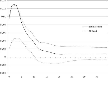
This bias-caused distortion can be seen in the results reported by Blanchard and Quah

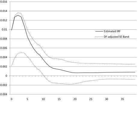
(1989); see especially their Figures 3 and 5. Our Figure 1 is a reestimated4 version of their Figure 3 with asymmetric one standard deviation bands.5 Notice that the upper one standard deviation band actually lies below the original estimated IRF over the early horizon interval.6 Anticipating our later discussion, Figure 2 shows the same impulse response function with one

       2

See, e.g., Runkle (1987) and Berkowitz and Kilian (2000).

3

This bias arises from the downward bias in the standard bootstrap estimate of the reduced form VAR error covariance matrix. Any object that depends on these estimates will be affected. This includes not only IRFs but bootstrap confidence intervals for error variance decompositions and bootstrap prediction intervals as well.

4

We make the same data adjustments made by Blanchard and Quah and estimate the model over the same sample period. Our results differ slightly because we use revised data.

5

We compute our asymmetric one standard deviation bands by obtaining 1000 bootstrap IRFs and then taking, in each direction, the square root of the mean squared deviation from the mean bootstrap IRF.

6

The fact that the corresponding Blanchard-Quah IRF does not actually cross the bounds is due to the way they compute their one standard deviation bands. They obtain 1000 bootstrap IRFs which, for each horizon, they

standard deviation bands after implementing a degrees of freedom adjustment to reduce bias.

The original asymmetry is greatly attenuated reflecting the fact that it is largely a spurious

consequence of bias in the bootstrap estimates of the IRF.

If, as in the case of Galí (1999), researchers do not allow for asymmetric confidence

intervals and simply plot error bands that are the estimated IRFs plus or minus one or two

standard deviations, then the CIs are symmetric by construction, any bias is completely invisible,

and the reported error bands are incorrect.7

Not all researchers attribute this seemingly odd behavior of IRFs completely to true

skewness. Christiano et al. (2006), for example, note that, in their case, the mean value of the

bootstrapped IRFs is quite different from the initial estimated IRF. They note that the

“asymmetric percentile confidence intervals show that when data are generated by these

[bootstrap] VARs, … the impulse response functions have a downward bias.”8

The finite-sample bias we examine arises from the fact that the bootstrap IRF for a

SVAR depends on the bootstrap OLS estimate of the error covariance matrix in the reduced

form vector autoregression (VAR), standard estimates of which are biased downward. This bias

is apparently common9 but, as we demonstrate below, it can be ameliorated by a degrees of freedom adjustment. Even though it can lead to substantially distorted bootstrap IRF CIs, this

bias is generally unrecognized and not corrected in practice because it only affects the bootstrap

estimates of the error variance, not the original OLS estimates.

Though the main insight of this paper is motivated by analogy to analytical results in a

simple regression model and confirmed by Monte Carlo evidence in more general settings, it is

important to indicate that the suggested degrees of freedom adjustment is ultimately inherently

heuristic since exact analytical underpinnings are not available in the case of a VAR model.

In the next section, we examine the specific source of this bias in the bootstrap estimate

of error variances in the context of a simple regression model and show how a degrees of

freedom adjustment eliminates the bias. We then consider autoregressive models. Since exact

finite-sample results are not available in this case, we proceed by analogy to suggest a similar       

7

This practice of forced symmetry is followed in some econometric software packages like EViews.

8

Christiano, Eichenbaum, and Vigfusson (2006), p. 26.

9

degrees of freedom adjustment and confirm its usefulness with Monte Carlo evidence. In

Section 3 we extend the analogy to show how the bias in bootstrap error variance estimates

effects the bootstrap IRFs and thus the bootstrap confidence intervals for the original IRF and,

again, suggest a degrees of freedom adjustment in this case of SVAR models. In Section 4 we

illustrate how making the recommended degrees of freedom adjustment affects the IRF

confidence intervals obtained in a widely-cited previous study. We also compare coverage rates

for the alternative bootstrap CIs. The final section offers a brief conclusion.

2. A SOURCE OF BIAS

2.1.Standard Regression Models

The simplest way to illustrate the bias under investigation is to examine a standard linear

regression model with nonstochastic regressors. We first consider a univariate regression model

represented by

(1) y Xu

where y is a T1 vector of observations on a dependent variable, X is a TR matrix of

observations on R nonstochastic regressors (perhaps including a constant),  is an R1 vector

of regression coefficients, and u is a T1 vector of errors. We assume that E u( )0 and

2

( ) T

E uu  I . Applying ordinary least squares (OLS), we obtain coefficient and error variance

estimates: ˆ (X X )1X y , ˆ2 1 (u uˆ ˆ) T R

  

 , where uˆ y Xˆ. The indicated degrees of

freedom correction makes 2 ˆ

 an unbiased estimator for 2 .

To help us understand the key argument to follow, it is useful to interpret the degrees of

freedom adjustment from the perspective that it is necessary to compensate for the fact that the

OLS residuals tend to be “smaller” than the error terms. Note that the expected value of the

average squared error is 2; i.e., E u u 2

T 



 _{ }

 

  . On the other hand,

ˆ ˆ

u u T R u u

E E

T T T

  

  _   

     

     , which reflects that, on average, the squared residuals are





       10

must rescale each residual by 1/ 2 T T R    _ 

  and then compute the average squared rescaled

residual giving the usual unbiased estimate for 2

, _ˆ2 1 _{ˆ ˆ} (u u) T R

  

 .

Now consider obtaining a bootstrap variance estimate in this simple case. The bootstrap

methodology relies on an analogy between the unknown population probability distribution of

the “real world” and the known empirical distribution in the “bootstrap world.”11 The bootstrap analyst hopes to learn about the population distribution of (ˆ22) by examining the

distribution of 2 _ˆ2

(  ) _where 2 ˆ

 _{is the “pseudo-population” variance of the empirical}

distribution (not a random variable in the bootstrap world) and _2

is a candidate bootstrap

variance estimate (which, of course, is a random variable in the bootstrap world).12 Typically, this is done by drawing many samples from the pseudo-population given by the original sample.

Because we can resample as many times as we want, we can estimate the mean of (2ˆ2)

and, thus, the bias of 2 using Monte Carlo experiments.

Pursuing this bootstrap analogy and recalling the insight discussed above, we might

expect an analogous degrees of freedom adjustment to be helpful for bootstrap variance

estimates. This has been confirmed for the simple regression model by Freedman and Peters

(1984, p. 99) and Peters and Freedman (1984, p. 408).

Suppose we obtain bootstrap estimates of the error variance as follows. For bootstrap

replications b=1,…, B, generate

(2) y_b* Xˆu*_b

where the elements of u_b* are drawn with replacement from the OLS residuals, ˆu. Then, apply

OLS to equation (2) to get bootstrap estimates of ˆ (not ), which we denote _b, and bootstrap

residuals, u_b. In the bootstrap, the variance estimate, 2

b

 , is an estimate of 2 ˆ

 (not 2 ), the

“population” error variance in the pseudo-population given by the original OLS residuals, ˆu.

The usual bootstrap variance estimate is given by 2 ,1

1

( )

b u ub b

T R  _      .        11

See Efron and Tibsharani (1993), especially Chapter 8, for discussion of this analogy.

12

So, in the bootstrap world, _2

is an estimate of _ˆ2

In this case, we can get some analytical insight for the properties of 2 ,1

_b by conditioning

on the unknown population distribution. Proceeding as above, we note that though

2 ˆ ˆ

u u E

T R 

  _{ }  _    , * * 2

b b b b

u u T R u u T R

E E

T R T T R T 

   _{  }    _{  }

  _{ }   _{ }

         

   

 

since the elements of u*_b are

drawn randomly from ˆu. This reflects that, on average, the squared bootstrap residuals are





Consequently, we suggest that a better bootstrap estimate might be given by

2 2

,2 2 ( ) ,1

( )

b b b b

T T

u u

T R T R

 _  _ 

 

    . This is the same rescaling suggested by Freedman and Peters

(1984) and Peters and Freedman (1984).

If this analogy holds exactly, we would expect the size of the (proportional) bias for the

natural estimator to be R T13. While this vanishes asymptotically, it can be important in small samples when R is large relative to T. To illustrate, we conduct a Monte Carlo experiment in

which we simulate obtaining bootstrap estimates of the error variance in a univariate regression

model like (1). We estimate models with nine regressors including a constant term, R9, for

three sample sizes: T 30, 50, 100.14 Consequently, the expected bias for _b2_,1 is -30%, -18% and -9% respectively. For each sample size, we draw 1000 samples of size T from a normal

distribution with mean zero and variance 0.81. For each of these Monte Carlo draws we generate

observations for y, estimate (1) by OLS, and compute the usual population-unbiased estimate of

the error variance, 2 ˆ

 . The average estimate is given in Table 1. To examine the bias of the two

       13

It should be noted that bias arising from maximum likelihood estimation (MLE) of the error variance will be even

larger. As is well known, the MLE of 2

, 2 1 

ˆ ˆ   u u

T , is biased; i.e.,

 

2 2

 _  _

 

 T R

E

T . Thus, the proportional

bias is R T. Now, when we bootstrap and obtain the MLE of _2

, 2_ 1

 

b u ub b

T , the bias is magnified since we

have a biased estimate of a biased estimate.  

2

2 2

( 2) 2

b   b T R

T , so

 

 2

2 2 2 b T R E T

    and the expected

proportional bias is  

2 2 2 2 2 1            

T R R TR

T T which is negative and larger (in absolute value) than 

R T.

14

The values of the regressors are 1.1, 1.0, 0.9, 0.8, o.7, 0.6, 0.5, 0.4, 0.3 with the first element being the constant term; 2

bootstrap error variance estimates, _b2_,1 and _b2_,2,15 we take each of the 1000 Monte Carlo samples and obtain 200 bootstrap estimates in each case. The average values are reported in

Table 1 for our three sample sizes. We call this the estimated bootstrap bias.

The results in Table 1 confirm our expectation very nicely. The “natural” bootstrap

estimator, _b2_,1, has bias approximately equal to R T while _b2_,2is approximately unbiased.

This bias in the standard bootstrap “error” variance carries over exactly to the case of a

multivariate seemingly unrelated regression model with nonstochastic regressors. To confirm

the theory, we have conducted simple Monte Carlo experiments similar to those undertaken for

the univariate regression model discussed above. To save space, we do not report the results

here but simply indicate that the conclusions are the same.16 2.2.Autoregressive Models

Consider a univariate AR(p) with a constant term, , so that R p 1:

(3) yt   ₁yt₁ ... pyt p ut; t  p 1,..., 0,1,...,T

where u_t is white noise with variance 2 and T is the number of usable observations. Because

the regressors are stochastic, the finite sample theory of the previous section does not apply.

However, following Stine (1987, p. 1074) and Berkowitz and Kilian (2000, p. 5), we might

speculate (correctly) that similar bias problems exist for bootstrap estimators of the error

variance in this case.

Since analytical results are not available, we examine the finite-sample bias issue for the

AR(p) model using a Monte Carlo exercise similar to the one described above. We generate

data for, and estimate, a model like (3) in which p8 so R9.17 For each of three sample sizes, T 30, 50, 100, we draw 1000 samples for u_t of size T+p from a normal distribution

with mean zero and variance 0.81. For each of these Monte Carlo draws we generate

observations for y, estimate (3) by OLS, and compute the usual estimate of the error variance,

2 ˆ

 . The average estimate is given in Table 2. To examine the bias (relative to ˆ2) of the two

bootstrap error variance estimates, _b2_,1 and _b2_,2, we obtain 200 bootstrap estimates for each of

       15

Note that Table 1reports the bias relative to, ˆ2, the pseudo-population variance.

16

The results are available on request.

17

The model coefficients are 0.008, 0.25, 0.11, -0.03, -0.004, -0.12, 0.03, -0.02, -0.08 with the first element being the constant term; 2

the Monte Carlo samples18. The average values are reported in Table 2 for each of our three sample sizes.

The results are quite informative. The heuristically expected bias for the corresponding

standard linear regression is a rather good guide for the bias in the AR(p) model. We confirm

that the bootstrap estimator of the error variance given by b2_,1 is biased and thus likely to result

in significant distortion when the number of slope coefficients is large relative to the sample size.

Proceeding by analogy, we expect these bias results to carry over to the case of a

(non-structural) VAR(p) with K variables. In that case, our interest is the K K error (innovation)

covariance matrix . Assuming a constant term, the usual degrees-of-freedom-corrected OLS

estimator for  is  ˆ  1  _ ˆ ˆ



T RU U where ˆUis the TKmatrix of OLS residuals and

1

 

R Kp . The “natural” but perhaps biased bootstrap estimator of ˆ is  _,1_ 1  _



   



b U Ub b

T R

where U_b is the TKmatrix of bootstrap residuals from the bth bootstrap iteration. The degrees

of freedom adjusted (DF-adjusted) bootstrap estimator of  is





,2  2

    _ _      

b b b

T

U U

T R

.

We have investigated the bootstrap error variance bias for a two-equation VAR(8) model

with a constant term using Monte Carlo methods similar to those described above and find the

bias to be quite close to the bias expected from the above heuristic analysis above. To conserve

space, we do not report the results here since they are quite similar to those reported for the

AR(8) model above.19 In particular, the bias for _b,1 is approximately Kp 1 T



 

_ _ where K is the

number of equations (variables) in the VAR(p). For a two-equation VAR(8) model, this implies

an approximate bias of -17% for each element of  when T 100.20

       18

For each bootstrap iteration, we obtain the initial p observations {y_{ p 1},...,y_o} by drawing (with replacement) from the original generated sample { }yt T p ₁.

19

Results are available on request.

20

3. BOOTSTRAPPING IRFS FOR SVARS

The downward bias of the standard bootstrap estimator of the VAR error covariance

matrix is of particular concern when we are interested in drawing inferences about IRFs from a

SVAR model since the IRFs are nonlinear functions of both VAR slope parameters and the

elements of the error covariance matrix.21 In this section we show how bias in the bootstrap estimate of the VAR error covariance matrix affects bootstrap IRFs and, thus, bootstrap CIs.

Consider a SVAR model explaining the behavior of a K1 vector of variables, y_t. The

IRFs are obtained from the moving average representation of the model:

(4) ( )y_t  A L_t

where _t is a vector of Kstructural shocks, L is the lag operator, and we make the standard

assumption that E( _{t t} ) I_K. This assumption provides a normalization as well as a set of

identifying restrictions. The elements of the matrix polynomial A L( ) give the impulse response

functions: a_{ij l,} ( ,i j1,... ;K l0,1,...) indicates the response of variable i in l periods to a one

unit (standard deviation) movement in the jth structural shock today. Though the IRFs are

frequently the objects of interest in macroeconomic analysis, they cannot generally be estimated

directly from time series data since the SVAR model (4) is not identified without further

restrictions.

To estimate the SVAR and thus the IRFs, we begin by specifying a finite-order reduced

form VAR model which can always be estimated:

(5) ( )B L y_t u_t

where B L( ) is a matrix of polynomials of order p and E u u( _{t t}  ) . In general, OLS estimates

of B L( ) and  can be obtained, B Lˆ ( ) and ˆ , where  ˆ  1  _ ˆ ˆ



T RU U, ˆUis the TKmatrix of

OLS residuals, and RKp1since we assume a constant term.

The reduced form moving average representation is obtained by inverting (5):

(6) y_t B L( )1u_t C L u( ) _t

       21

where C₀ I, the identity matrix. Equating terms in (4) and (6) allows us to conclude the

following:

(7) u_t  A₀_t

(8) A_l C A_{l 0} l1,...

Thus, it is clear that knowledge of the K2 elements ofA₀ is sufficient to obtain the IRF.

From (7) we infer the key relationship between the covariance matrices of the structural

and reduced form errors:

(9)   A A_{0 0}

Symmetry of  provides ( 1) 2 K K

 

 

  restrictions on A0. With

( 1) 2 K K

 

 

  additional

restrictions, A₀ can be identified and IRFs computed. Equations (8) and (9) assure us that the

estimated IRFs depend on the estimates of both B L( ) and . I.e.,

, ˆ

ˆ_{ij l} ( , ) ( ,ˆ 1,... ; 1,...)

a g   i j  K l where ˆ vec B( )ˆ , a K Kp(  1) 1 vector, and ˆ vech( )ˆ

, a ( 1) 1 2

K K

 _

 

  vector and the form of the nonlinear function g depends on the identification

strategy. Consequently, the properties of the IRFs depend on the properties of ˆ and ˆ .

Similarly, the properties of the bootstrap IRFs depend in the same way on the properties of the

bootstrap estimates of  and : aij l_, g( , ) ( ,   i j1,... ;K l0,1,...).

We can see from this that there are several potential sources of bias for the bootstrapped

IRFs and, thus, bootstrap confidence intervals for the original IRFs. The source we focus on

here arises when the bootstrap estimate of , , is biased for ˆ , the elements of the

pseudo-population covariance matrix. How much difference does the appropriate degrees or freedom

adjusted bootstrap estimation of the error covariance matrix make for bootstrap estimates of the

IRF? We provide some intuitive analytics to address this question.

From equation (8) we infer that the bootstrap estimates of the IRF are given by

(10) A_l C A _{l 0} l1,...

where A_l, C_l, and A₀ are bootstrap estimates. Any bias in A₀ will, thus, likely carry over to all

which, based on results reported above, we expect to be systematically biased. Consequently, it

will be instructive to consider how potential bias in the bootstrapped estimates of the VAR

covariance matrix can affect the bootstrapped IRF.

The original sample estimate of the VAR error covariance matrix is  ˆ  1  _ ˆ ˆ



T RU U.

As in the previous section, we consider two alternative bootstrap estimates of ˆ based on the

pseudo-population. The standard bootstrap estimate is given by  _,1 _ 1  _



   



b U Ub b

T R where Ub



is the TKmatrix of bootstrap residuals from the bth bootstrap iteration. The DF-adjusted

bootstrap estimate is given by  _,2 _{ } 1 _  _ _ _,1

  

      

 

b b b b

T T

U U

T R T R T R . So,

(11) _b,1  1b _b,2

where b R

T is the proportional difference between the standard and DF-adjusted bootstrap

estimates of ˆ . Based on the results of the previous section (including the Monte Carlo

evidence alluded to), we might expect b to approximate the bias in _b,1.

We can use equation (11) to derive the implied proportional difference between the

corresponding bootstrapped IRFs. Equation (9) implies that  _b,1 A A_0,1_0,1 and  _b,2 A A_0,2_0,2.

So, from (11) we have A A _{0,1 0,1}  (1 b A A)_0,2 _0,2 which, in turn, implies that

(12) A_0,1 (1 b)1/ 2A_0,2  (1 a A)_0,2

Equating (1b)1/ 2 and (1a) in (12) implies that b and a are related by

(13) a (1 b)1/ 21

Since     1 b R 0

T , we see that b a 0 .

Now, consider how this proportional difference in the bootstrap estimate of Aˆ₀ affects

the alternative bootstrap IRFs. First, it is important to recognize that C_l does not depend on

which bootstrap estimate of ˆ we choose. Thus, as implied by equation (10), the two IRFs are

(14) Al j_, C A l _0,j j1, 2; l1,...

In particular,

(15) _{,2 0,2} 1 _0,1 1 _,1

1 1

   

  _{ } _{ }

 

   

     

l l l l

A C A C A A

a a

where the second equality follows from (12) and the final equality follows from (14). From

equation (15), it follows that the proportional difference between the two IRFs is the same for all

values of l:

(16) ,1 ,2 ,2

, 1,...



 

 



l l l

A A

a l

A .

Thus, the bootstrap IRF proportional difference is constant and equal to a for the entire

IRF horizon. So, for example, if we have a SVAR model with K=2, p=8, T=100 and a constant

term, the elements of the standard bootstrap covariance matrix estimate is 17% less than the

DF-adjusted estimate and the corresponding IRFs differ by 9% of the DF-DF-adjusted IRF.22

4. An Example

As indicated earlier,23 the procedures that generate this bias seem to be quite common in the empirical SVAR literature. In this section we illustrate its effect in practice by replicating the

biased results obtained in a single influential paper by Chistiano et al. (1999). We then compute

the corresponding DF-adjusted IRF and associated bootstrap confidence intervals to draw our

comparison. Finally, we examine coverage accuracy by comparing the coverage rates for

standard bootstrap CIs with those for the DF-adjusted CI.

In their paper, Chistiano et al.xamine the effects of monetary policy shocks on several

economic variables of interest using models imposing a recursive structure to identify the

relevant shocks. Their first benchmark model includes a constant term and four lags (p=4) of

seven variables (K=7) with the federal funds rate as the chosen monetary policy instrument.

They estimate their models using quarterly data over the period 1965:3-1995:2. Given the loss

of observations due to the four lags in the VAR, T=116 in our notation. We replicate their       

22

These are the implied values of band a in percentage terms. As indicated above, b R

T , and a can be

computed from (13).

23

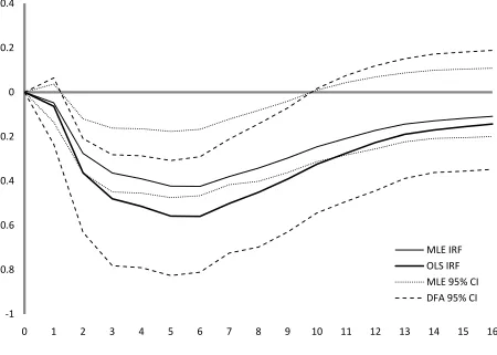
results by estimating their model over the same sample period.24 For illustrative purposes, we report only the IRF indicating the effects of a negative monetary policy shock on output. While

this is an IRF of particular interest, the same bias will be present in all the other 48 IRFs as

well.25 As seen in Figure 3 here and Figure 2 of CEE (1999, p. 86), given a positive federal funds rate shock, “after a delay of 2 quarters, there is a sustained decline in real GDP ” (p. 87).

We note that CEE use MLE to estimate the VAR error covariance estimate so the estimated IRF

will be biased. Furthermore, we see that the bootstrap confidence intervals reflect considerable

asymmetry which, we shall see momentarily, is partially due to bias in the confidence intervals

arising from biased bootstrap IRF estimates.

To illustrate the effect of bias due to MLE and the further bias due to the CEE bootstrap

IRFs, we estimate the CEE model once again but this time including the degrees of freedom

correction we suggest in this paper. These results for the first-stage IRF and the bootstrap

confidence intervals are also reported in Figure 3. We first notice that the fundamental

conclusion regarding the IRF is unchanged: a contractionary federal funds rate shock will, after a

lag, have a sustained negative effect on real GDP.26 We also notice that adjusting the degrees of freedom in the original error covariance matrix estimate causes the corresponding IRF to lie

entirely below the CEE IRF.

In addition, we see that the confidence intervals also shift significantly when we adjust

the degrees of freedom in the bootstrap estimates of the error covariance matrix. We note three

consequences. First, we see that for much of the time horizon, the DF-adjusted OLS IRF

actually lies below the CEE 95% confidence intervals. Second, we see that adjusting the degrees

of freedom has greatly reduced the asymmetry in the confidence intervals.27 Third, we notice       

24

Indeed, we have estimated the CEE model using their data which Larry Christiano has generously made available on his website.

25

This is because, as equation (12) shows, the proportional difference between the bootstrap estimates of the A₀

matrix is a multiplicative scalar that affects all elements of the matrix the same way. Equation (14) shows that this same proportional difference will carry over to every IRF.

26

Indeed, we will always draw the same conclusion about statistical significance when our interest is in whether or not the IRF is significantly different from zero. This is a consequence of the fact, illustrated in the previous section equation (15), that the DF-adjusted bootstrap IRF is proportional to the standard IRF at all horizons with the constant of proportionality positive but less than one. Accordingly, both confidence interval bounds will cross the horizontal axis (zero line) at exactly the same horizons. This implies that the range over which the IRF is

significantly greater or less than zero will be the same whether or not a degrees of freedom adjustment is applied. Adjusting the degrees of freedom can lead to a reversal of conclusion, however, if the null hypothesis takes on a value other than zero.

27

that between 2 and 11 quarters, the upper 95% confidence bounds are farther away from zero

after degrees of freedom adjustment. This provides stronger evidence supporting the conclusion

that a contractionary monetary policy has a significant negative effect on output over that

horizon.

Since part of the distortion in the CEE results is a consequence of their choice to use

MLE estimates of the error covariance matrix, we also illustrate how much distortion remains

when we use OLS estimates. The results are reported in Figure 4. In the typical approach

incorporating the natural OLS degrees of freedom correction, the original IRF is already

DF-adjusted so we only have a single IRF estimate. However, the typical procedure does result in

biased bootstrap confidence intervals. As in Figure 3, we again see that the typical biased

procedure results in quite asymmetric confidence intervals which are, in part, a consequence of

the bias; the DF-adjusted confidence intervals exhibit much less asymmetry. Also, as noted in

the discussion of Figure 3, over a range of intermediate horizons, the upper bound of the

DF-adjusted confidence intervals lie below their biased counterparts giving us greater confidence in

our conclusion that a monetary contraction has a significant negative effect on output.

These examples illustrate that adjusting the degrees of freedom in both the original IRF

and especially in the bootstrap confidence interval estimates can remove distortions that change

the quantitative (if not qualitative) conclusions when SVAR models are used.

Of course, for the degrees of freedom adjustment we recommend to be of practical value,

we must have confidence that it will result in greater coverage accuracy for the resulting CIs.

Accordingly, we conclude this section by reporting the results of a series of Monte Carlo

experiments that investigate the coverage rates of alternative bootstrap CIs. To avoid the

potential arbitrariness of an ad hoc data generating process (DGP), we treat the benchmark CEE

model as our initial DGP from which we obtain the “true” IRF.28 Using that model and assuming jointly normal errors with the CEE estimated covariance matrix, we generate 1000

Monte Carlo trials of the same length as the CEE sample. Once again, to keep the analysis

focused, we look only at the IRF representing the effect of a negative monetary policy shock on

       28

Kilian and Chang (2000) argue that the results of studies that focus on simple ad hoc (e.g., bivariate) VAR models may not generalize to higher dimensional models that are typical of actual applied work. In their study investigating coverage rates, they use three leading models in the literature, including the CEE model, as data generating

output.29 For each Monte Carlo trial, we then take 200 bootstrap replications and construct three sets of 95% bootstrap IRF confidence intervals: MLE (following CEE), standard OLS, and

DF-adjusted. We then report the coverage rates30 for each of these respective confidence intervals across the 1000 trials.

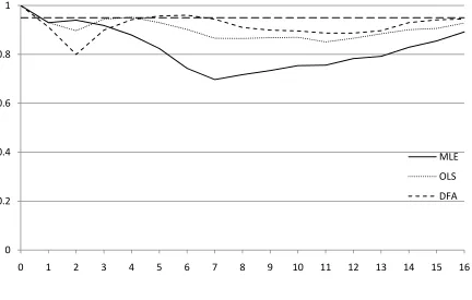
Figure 5 reports the results for the benchmark CEE model DGP along with a reference

line at 0.95 reflecting the 95% nominal value of the confidence intervals. We label the methods:

MLE, OLS, and DFA. We notice that none of the methods yield coverage rates that are

consistently near the ideal value of 0.95 but the DFA method we recommended is uniformly

superior to the traditionally-used alternatives. Coverage rates for the DFA method fall to about

0.6 but are generally above 0.7. The MLE has particularly poor coverage rates for intermediate

horizons, falling as low as 0.2 while coverage rates fall in between for the OLS method.

To get some idea regarding the robustness of the finding that the DFA method gives

greater coverage accuracy, we consider alternative parameterizations of the benchmark CEE

model. Because of the impracticality of varying the very large number of slope parameters for

the seven-equation, four-lag CEE model in any systematic way, we have chosen to pursue some

alternative parameterizations of the covariance matrix instead. The first of these alternatives

doubles all the values of the elements of the estimated covariance matrix, the second halves those

values, and the third sets all the off-diagonal elements to zero. The results are reported in

Figures 6 through 8.

As reported in Figure 6, for the model with a doubled covariance matrix, the coverage

rates for all methods improve considerably with the DFA method generally but not always being

closer to the ideal value. The average coverage rate across all horizons is 0.913 for DFA, 0.898

for OLS, and 0.814 for MLE. It appears that all methods do better in the face of larger variances.

We find the complement of the above results when the variances are halved (Figure 7).

None of the methods show much coverage accuracy even though the DFA method is uniformly

superior.

Finally, when we set all covariance values to zero, the results are very similar to those of

the benchmark model including the superiority of the DFA method (see Figure 8). This

similarity is a consequence of the fact that the estimated covariances are generally small.

       29

For comparison, see the upper left graph in Figure 3 of Kilian and Chang (2000).

30

5. Conclusion

This paper has discussed a commonly occurring source of bias in bootstrap estimates of

confidence intervals for IRFs in SVARs arising from the downward bias in the traditional

bootstrap estimate of the VAR covariance matrix. Since the bootstrap IRFs depend on these

biased estimates, they are systematically distorted along with the implied bootstrap IRF

percentile confidence intervals. This distortion is potentially large but, fortunately, can be

readily ameliorated by an additional degrees of freedom adjustment when estimating the VAR

covariance matrix. Furthermore, the results of a series of Monte Carlo experiments suggest that

we can expect the degrees of freedom adjusted confidence intervals to exhibit improved

References

Berkowitz, J., Kilian, L., 2000. Recent developments in bootstrapping time series. Econometric Reviews 19, 1-48.

Blanchard, O., Quah, D., 1989. The dynamic effects of aggregate demand and supply disturbances. American Economic Review 79, 655-673.

Christiano, L. J., Eichenbaum, M., Evans, C. L., 1999. Monetary policy shocks: What have we learned and to what end?, in: Taylor, J.B., Woodford, M., (Eds.) The Handbook of Macroeconomics, vol. 1. North Holland, Amsterdam, pp. 65-148.

Christiano, L. J., Eichebaum, M., Vigfusson, R., 2006. Assessing structural VARs. NBER Macroeconomics Annual 21, 1-72.

Davidson, R., MacKinnon, J. G., 1993. Estimation and inference in econometrics. Oxford University Press, New York.

Efron, B., Tibshirani, R. J., 1993. An introduction to the bootstrap. Chapman & Hall, New York.

Freedman, D. A., Peters, S. C., 1984. Bootstrapping a regression equation: Some empirical results. Journal of the American Statistical Association 79, 97-206.

Galí, J., 1999. Technology, employment, and the business cycle: Do technology shocks explain aggregate fluctuations? American Economic Review 89, 249-271.

Kilian, L., Chang, P., 2000. How accurate are confidence intervals for impulse responses in large VAR models? Economics Letters 69, 299-307.

Inoue, A., Kilian, L., 2002. Bootstrapping smooth functions of slope parameters and innovation variances in VAR(∞) models. International Economic Review 43, 309-331.

Peters, S. C., Freedman, D. A., 1984. Some notes on the bootstrap in regression problems. Journal of Business and Economics Statistics 2, 406-409.

Runkle, D. E., 1987. Vector autoregression and reality. Journal of Business and Economics Statistics 5, 437-442.

Sims, C. A., Zha, T., 1999. Error bands for impulse responses. Econometrica 67, 1113-1155.

Table 1: Bootstrap error variance estimates in standard univariate linear regression model with R=9; number of Monte Carlo trials = 1000, number of bootstrap draws = 200. True value of variance =0.81.

Estimator Sample Size Mean Estimate Expected Bias Estimated Bootstrap Bias

2 ˆ

 30 0.8051

2 (1)

b

 30 0.5633 -30.0% -30.03%

2 (2)

b

 30 0.8047 0 -0.05%

2 ˆ

 50 0.8053

2 (1)

b

 50 0.6603 -18.0 % -18.01%

2 (2)

b

 50 0.8053 0 0.00%

2 ˆ

 100 0.8054

2 (1)

b

 100 0.7327 -9.0% -9.03%

2 (2)

b

 100 0.8052 0 -0.02%

a_{The estimated bootstrap bias is the average difference between the relevant bootstrap error variance}

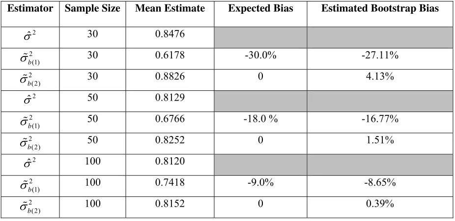
Table 2: Bootstrap error variance estimates in an AR(8) model with a constant term (R=9); number of Monte Carlo trials = 1000, number of bootstrap draws = 200. True value of variance =0.81.

Estimator Sample Size Mean Estimate Expected Bias Estimated Bootstrap Bias

2 ˆ

 30 0.8476

2 (1)

b

 30 0.6178 -30.0% -27.11%

2 (2)

b

 30 0.8826 0 4.13%

2 ˆ

 50 0.8129

2 (1)

b

 50 0.6766 -18.0 % -16.77%

2 (2)

b

 50 0.8252 0 1.51%

2 ˆ

 100 0.8120

2 (1)

b

 100 0.7418 -9.0% -8.65%

2 (2)

b

 100 0.8152 0 0.39%

a_{The estimated bootstrap bias is the average difference between the relevant bootstrap error variance}

Figure 1: A reestimated version of Figure 3 in Blanchard and Quah (1989). It shows the response of output to aggregate demand shocks with asymmetric one standard deviation bands based on standard bootstrap estimates.

‐0.004

‐0.002 0 0.002 0.004 0.006 0.008 0.01 0.012 0.014

0 5 10 15 20 25 30 35

Estimated IRF

Figure 2: A reestimated version of Figure 3 in Blanchard and Quah (1989) with asymmetric one standard deviation bands based on degrees of freedom adjusted bootstrap estimates.

‐0.004

‐0.002 0 0.002 0.004 0.006 0.008 0.01 0.012 0.014 0.016

0 5 10 15 20 25 30 35

Estimated IRF

Figure 3: Impulse response functions showing the effect of a contractionary monetary policy on real GDP with 95% confidence intervals. The solid line gives the original MLE IRF and the long-dashed bold line gives the OLS IRF; CEE use MLE. The dotted lines give the MLE bootstrap 95% confidence intervals and the dashed lines give the DF-adjusted 95% confidence intervals.

‐1

‐0.8

‐0.6

‐0.4

‐0.2 0 0.2 0.4

0 1 2 3 4 5 6 7 8 9 10 11 12 13 14 15 16

MLE IRF OLS IRF

MLE 95% CI

‐1

‐0.8

‐0.6

‐0.4

‐0.2 0 0.2 0.4

0 1 2 3 4 5 6 7 8 9 10 11 12 13 14 15

MLE IRF OLS IRF CMLE 95% CI DFA 95% CI

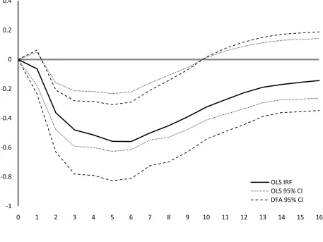
Figure 4: Impulse response function showing the effect of a contractionary monetary policy on real GDP with 95% confidence intervals. The solid line gives the original OLS IRF. The dotted lines give the typical bootstrap 95% confidence intervals not adjusted for degrees of freedom and the dashed lines give the DF-adjusted 95% confidence intervals.

‐1

‐0.8

‐0.6

‐0.4

‐0.2 0 0.2 0.4

0 1 2 3 4 5 6 7 8 9 10 11 12 13 14 15 16

Figure 5: Coverage rates for MLE, OLS, and DFA bootstrap 95% CIs applied to the CEE model as originally parameterized.

0 0.2 0.4 0.6 0.8 1

0 1 2 3 4 5 6 7 8 9 10 11 12 13 14 15 16

MLE

OLS

Figure 6: Coverage rates for MLE, OLS, and DFA bootstrap 95% CIs applied to the CEE model with a doubled covariance matrix.

0 0.2 0.4 0.6 0.8 1

0 1 2 3 4 5 6 7 8 9 10 11 12 13 14 15 16

MLE

OLS

Figure 7: Coverage rates for MLE, OLS, and DFA bootstrap 95% CIs applied to the CEE model with all elements of the covariance matrix halved.

0 0.2 0.4 0.6 0.8 1

0 1 2 3 4 5 6 7 8 9 10 11 12 13 14 15 16

MLE

OLS

Figure 8: Coverage rates for MLE, OLS, and DFA bootstrap 95% CIs applied to the CEE model with all off-diagonal elements of the covariance matrix set to zero.

0 0.2 0.4 0.6 0.8 1

0 1 2 3 4 5 6 7 8 9 10 11 12 13 14 15 16

MLE

OLS