Mean Square Solutions of Second Order Random Differential Equations by Using the Differential Transformation Method

http://dx.doi.org/10.4236/ojapps.2016.64028

Mean Square Solutions of Second-Order

Random Differential Equations by Using the

Differential Transformation Method

Ayad R. Khudair, S. A. M. Haddad, Sanaa L. Khalaf

Department of Mathematics, Faculty of Science, University of Basrah, Basrah, Iraq

Received 21 March 2016; accepted 25 April 2016; published 28 April 2016

Copyright © 2016 by authors and Scientific Research Publishing Inc.

This work is licensed under the Creative Commons Attribution International License (CC BY).

http://creativecommons.org/licenses/by/4.0/

Abstract

The differential transformation method (DTM) is applied to solve the second-order random diffe-rential equations. Several examples are represented to demonstrate the effectiveness of the pro-posed method. The results show that DTM is an efficient and accurate technique for finding exact and approximate solutions.

Keywords

Random Differential Equations, Stochastic Differential Equation, Differential Transformation Method

1. Introduction

The ordinary differential equations which contain random constant or random variables are well known topics which are called the random ordinary differential equations. The subject of second-order random differential equations is one of much current interests due to the great importance of many applications in engineering, bi-ology and physical phenomena (see, e.g. Chil’es and Delfiner [1], Cort’es et al. [2], Soong [3] and references therein). Recently, several first-order random differential models have been solved by using the Mean Square Calculus [2] [4]-[11]. Variety scientific problems have been modeled by using the nonlinear second-or- der random differential equations. However, most of these equations cannot be solved analytically. Thus, accu-rate and efficient numerical techniques are needed. There are several semi-numerical techniques which have been considered to obtain exact and approximate solutions of linear and nonlinear differential equations, such as adomian decomposition method (ADM) [12], variational iteration method (VIM) [13] and homotopy perturba-tion method (HPM) [14]. We observe that semi-numerical methods are very prevalent in the current literature, cf. [12]-[14].

finding exact and approximate solutions of the second-order random differential equations. To this end, the second-order random differential equations and the concept of the differential transformation method are pre-sented in Section 2. In Section 3, we consider the statistical functions of the mean square solution of the second- order random differential equation. Section 4 is devoted to numerical examples.

2. Differential Transform Method

The differential transform method (DTM) has been used by Zhou [15]. This method is effective to obtain exact and approximate solutions of linear and nonlinear differential equations. To describe the basic ideas of DTM, we consider the second order random differential equation,

( )

( )

,

( )

,

L x t_ _+N x t_ A_=g t (1)

( )

0

( )

1

0 d 0 , d t x t

x y y

t ₌

= = (2)

where

( )

( )

2 2

d

d

x t L x t

t

=

 

  , x t

( )

is an unknown function, N x t_

( )

,A_ is a nonlinear operator, g t

( )

is the source in homogeneos term, and A y, 0 and y1 are random variables.

We now write the differential transform of function as

( )

( )

0 d 1 ! d k k t x t X k

k t ₌

= (3)

In fact, x t

( )

is a differential inverse transform of the form

( )

( )

0

k k

x t X k t

∞

=

=

∑

(4)

It is clear from (3) and (4) that the concept of differential transform is derived from Taylor series expansion. That is

( )

( )

0 0 d 1 ! d k k k k t x t

x t t

k t

∞

= ₌

=

∑

(5)

Original function Transformed function

( ) ( )

x t ±y t X k( )±Y k( )

( )

cx t cX k( )

( ) d ( ) d

x t y t

t

= Y k( ) (= k+1) (X k+1)

( ) 2 ( )2 d

d

x t y t

t

= Y k( ) (= k+1)(k+2) (X k+2)

( ) ( ) ( )

u t =x t y t ( ) ( ) ( )

0

k

s

U k X s Y k s

=

=

∑

−

( ) s

x t =t ( ) 1

0 k s X k k s =  =  _≠  ( ) d ( )

d

x t y t t

t

= Y k( )=kX k( )

( ) 2 ( )2 d

d

x t y t t

t

= Y k( )=k k( +1) (X k+1)

( ) 2 2 ( ) 2 d

d

x t y t t

t

= Y k( )=k k( −1) ( )X k

Notes that, the derivatives in differential transform method does not evaluate symbolically.

In keeping with Equations (3) and (4), let X k

( )

, Y k

( )

and U k

( )

, respectively, are the transformed

func-tions of x t

( )

, y t

( )

and u t

( )

. The fundamental mathematical operations of differential transformation are listed in the following table.

3. Statistical Functions of the Mean Square Solution

Before proceeding to find the computation of the main statistical functions of the mean square solution of Equa-tions (1) and (2) we briefly clarify some concept, notation, and results belonging to the so-called LP calculus. The reader is referred to the books by Soong [3], Loeve [16], and Wong and Hajek [17]. Throughout the paper, we deal with the triplet Probabilistic space

(

Ω, ,F P

)

. Thus, suppose L2=L2

(

Ω, ,F P

)

is the set of second order random variables. Then the random variable X:Ω → ∈R L2, if

2

E X_  < ∞_ , where E

[ ]

 is an ex-pectation operator. The norm on is denoted by

2

 . For example, for the random variable X we define

(

)

1

2 2 2

X = E X_ _ , in such way that

(

L2, X 2

)

is a Banach space. In addition, let T (real interval) represent

the space of times, we say that

{

X t t

( )

, ∈T

}

is a second order stochastic process, if the random variable

( )

2

X t ∈L for each t∈T.

A sequence of second order random variables

{

X_n,n≥0

}

converges to X t

( )

∈L2, if

1 2 ₂

lim n lim n 0.

n→∞ X X n→∞ E X X

 _{ } 

− =  _ − _ =

 

To proceed from (4), we truncate the expansion of at the term as follows

0 ( ) ( ) N k N k

x t X k t

=

=

∑

(6)

By using the independence between A y, 0 and y1 we have

( )

( )

0 N k N k

E x t E X k t

=

=

   

 

∑

  (7)

( )

(

( ) ( )

)

0 0 cov , N N i j N j i

V x t X i X j t+

= =

=

 

 

∑∑

(8)

where cov

(

X i

( ) ( )

,X j

)

=E X i X j

(

( ) ( )

)

−E X i_

( )

_{ } E X j

( )

_,∀i j, =0,1,,N.

The following Lemma guarantee the convergent of the sequence E X_ _N

( )

t _ to E X t_

( )

_ and the se-quenceV X_{ N}

( )

t _ to V X t_

( )

_ if the sequence the X_N

( )

t converges to X t

( )

.

Lemma [5]: Let

{ }

X_N and

{ }

Y_N be two sequences of 2-r.vs X and Y, respectively, i.e., lim _N

N→∞X =X and

lim _N

N→∞Y =Y then Nlim→∞E X Y

[

N N

]

=E XY

[ ]

. If XN =YN, then

2 2

lim _N

N→∞E X E X

 =  

   , lim

[ ]

N

[ ]

N→∞E X =E X and lim

[ ]

_N

[ ]

N→∞V X =V X .

4. Numerical Examples

In this section, we adopt several examples to illustrate the using of differential transform method for approx-imating the mean and the variance.

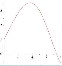
Example 1: Consider random initial value problem

( )

( )

2 2 2 d 0 d x t

A x t

t + = , x

( )

0 =Y0 and

( )

1 0 d d _t x t Y

t ₌ =

where A2Be

(

α =2,β =1

)

and independently of the initial conditions Y0 and Y1 which satisfy E Y

[ ]

o =1,

2

2 o

E Y  =_{ } , E Y

[ ]

1 =1,

2

1 3

E Y  =_{ } and E Y Y

[ ]

0 1 =0. The approximate mean and variance are

( )

1 2 1 3 1 4 1 5 1 6 1 7 1 8

1

3 9 48 240 1800 12600 120960

( )

4 2 8 3 19 4 67 5 103 6 41 7 247 8

1 2

3 9 72 540 4050 4725 172800

V x t_ _= − +t t + t − t − t + t + t − t −

Figure 1 explain the Graph of the expectation approximation solution by using DTM with n = 18, while Fig-ure 2 explain the Graph of variance approximation solution by using DTM with n = 18.

Example 2: Consider random initial value problem

( )

( )

2 2 d 0 d x t Atx t

t + = , X

( )

0 =Y0 and

( )

1 0 d d t x t Y t ₌ = where A is a Beta r.v. with parameters α =2 and β =3, i.e. ABe

(

α =2,β=3

)

and the initial conditions

o

Y and Y1 are independent r.v.’s such as E Y

[ ]

o =1,

2 2

o

E Y  =_{ } , E Y

[ ]

1 =2, 2

1 5

E Y  =_{ } . The approximate mean and variance are

( )

1 3 1 4 1 6 1 7 1 9 1 10

1 2

15 15 900 1260 113400 198450

E x t_ _= + −t t − t + t + t − t − t +

( )

2 2 3 1 5 2 6 1 7 83 8 83 9 2 10

1

15 15 225 450 25200 283500 18375

V x t_ _= + −t t − t + t + t + t − t − t −

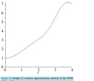
Figure 3 explain the Graph of the expectation approximation solution by using DTM with n = 18, while Fig-ure 4 explain the Graph of variance approximation solution by using DTM with n = 18.

Example 3: Consider the problem

( )

( )

( )

2 2 2 d d 2 0 d d

x t x t

A A x t

t

t + + = , x

( )

0 =Y0 and

( )

1 0 d d t x t Y

t ₌ = where

A is a Beta r.v. with parameters α =2 and β =1, i.e. ABe

(

α=2,β=1

)

and independently of the initial conditions Yo and Y1 which are independent r.v.’ satisfy E Y

[ ]

o =1,

2 2

o

E Y  =_{ } , E Y

[ ]

1 =1, 2

1 1

E Y  =_{ } . The approximate mean and variance are

( )

11 2 23 3 13 4 59 5 83 6 37 7 143 8

1

12 60 120 2520 20160 60480 1814400

E x t_ _= + −t t + t − t + t − t + t − t +

Figure 1. Graphs of the expectation approximation solution of the

DTM with n = 18.

1 2 3 4 5 6 7 8

[image:4.595.131.505.388.698.2]

[image:5.595.181.441.81.361.2] [image:5.595.185.444.381.659.2]

Figure 2. Graphs of variance approximation solution of the DTM with n = 18.

Figure 3. Graphs of the expectation approximation solution of the

DTM with n = 18.

( )

1 2 4 3 103 4 649 5 8959 6 3133 7 517 8

1

2 15 720 2520 50400 37800 17280

V x t_ _= − t + t + t − t + t − t + t −

0 1 2 3 4 5 6

t

4

3

2

1

t

0

3

2

1

[image:6.595.187.510.82.361.2]

Figure 4. Graphs of variance approximation solution of the DTM with n = 18.

Figure 5 explain the Graph of the expectation approximation solution by using DTM with n = 18, while Fig-ure 6explain the Graph of variance approximation solution by using DTM with n = 18.

Example 4: Consider the problem

( )

( )

2 2 d 0 d x t Atx t

t + = , X

( )

0 =Y0 and

( )

1 0 d d t x t Y

t ₌ = where A is a uniform r.v. with parameters α =0 and β =1, i.e. AU

(

α =0,β =1

)

and independently of the initial conditions Yo and Y1 which are independent r.v.’s satisfy E Y

[ ]

o =1,

2 ₂

o

E Y  =_{ } , E Y

[ ]

1 =1, 2

1 1

E Y  =_{ } . The approximate mean and variance are

( )

11 2 23 3 13 4 59 5 83 6 37 7 143 8

1

12 60 120 2520 20160 60480 1814400

E x t_ _= + −t t + t − t + t − t + t − t +

( )

1 6 1 8 131 10 41 12 71471 14

1

432 1440 1008000 2177280 31294771200

V x t_ _= + t − t + t − t + t 

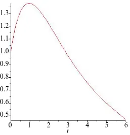
Figure 7 explain the Graph of the expectation approximation solution by using DTM with n = 18, while Fig-ure 8 explain the Graph of variance approximation solution by using DTM with n = 18.

Example 5: Consider the problem

( )

( )

2 2 d 0 d x t Ax t

t + = , X

( )

0 =Y0 and

( )

1 0 d d t x t Y

t ₌ = where A is a uniform r.v. with parameters α =0 and β =2, i.e. AU

(

α=0,β =2

)

and independently of the initial conditions Yo and Y1 which are independent r.v.’s satisfy E Y

[ ]

o =1,

2 ₄

o

E Y  =_{ } , E Y

[ ]

1 =1, 2

1 2

E Y  =_{ } . The approximate mean and variance are

( )

1 2 1 3 1 4 1 5 1 6 1 7 1 8 1 9

1

2 6 18 90 360 2520 12600 113400

E x t_ _= + −t t − t + t + t − t − t + t + t −

( )

2 13 4 1 5 61 6 2 7 599 8 101 9

3 2

12 18 270 135 22680 56700

V x t_ _= − t + t + t − t − t + t + t −

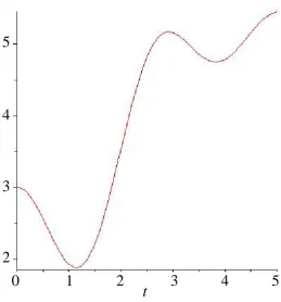
Figure 9 explain the Graph of the expectation approximation solution by using DTM with n = 18, while Fig-ure 10 explain the Graph of variance approximation solution by using DTM with n = 18.

t

7

6

5

4

3

2

1

0

[image:7.595.188.445.80.346.2] [image:7.595.186.443.377.644.2]

Figure 5. Graphs of the expectation approximation solution of the HAM with n = 18.

Figure 6. Graphs of variance approximation solution of the HAM

with n = 18.

Example 6: Consider the problem

( )

( )

( )

( )

2 2

d

sin d

x t

Ax t x t t

t + = − + , x

( )

0 =Y0 and

( )

1 0

d d _t

X t Y

t ₌ = where

A is a uniform r.v. with parameters α =1 and β =2, i.e. AU

(

α =1,β =2

)

and independently of the

t

0 1 2 3 4 5 6

1.3

1.2

1.1

1.0

0.9

0.8

0.7

0.6

0.5

t

0 1 2 3 4 5 6

1.0

0.9

0.8

[image:8.595.185.466.82.352.2]

Figure 7. Graphs of the expectation approximation solution of the DTM with n = 18.

Figure 8. Graphs of variance approximation solution of the DTM with

n = 18.

initial conditions Yo and Y1 which satisfy E Y

[ ]

o =1,

2 2

o

E Y  =_{ } , E Y

[ ]

1 =1, 2

1 6

E Y  =_{ } and E Y Y

[ ]

0 1 =0. The approximate mean and variance are

t

0 1 2 3 4

0

3

2

1

t

0 1 2 3 4

1.4

1.2

1.0

0.8

0.6

0.4

0.2

[image:8.595.187.445.384.653.2]

[image:9.595.190.444.86.349.2]

Figure 9. Graphs of the expectation approximation solution of the DTM with n = 18.

Figure 10. Graphs of variance approximation solution of the DTM

with n = 18.

( )

₁ 5 2 1 3 19 4 17 5 13 6 11 7 211 8

4 4 72 720 576 8640 201600

E x t_ _= + −t t − t + t + t − t − t + t +

1 2 3 4 5

t

1.4

1.2

1.0

0.8

0.6

0.4

0.2

0

−0.2

5

t

0 1 2 3 4 5

4

3

[image:9.595.183.443.377.656.2]

( )

_{1 2} 5 2 10 3 293 4 67 5 185 6 12221 7 198419 8

2 3 144 40 288 30240 1814400

V x t_ _= − t+ t + t − t − t + t + t − t −

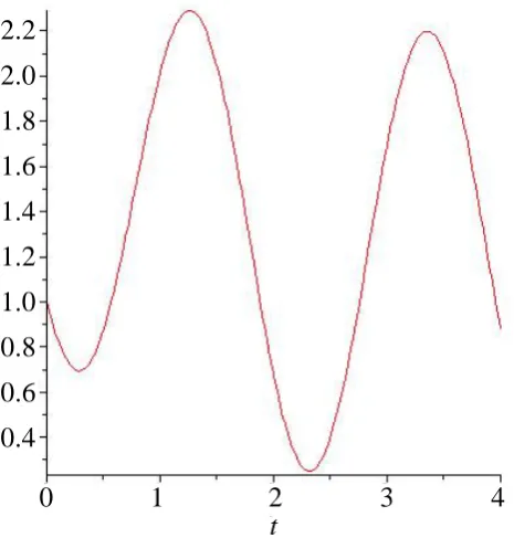
Figure 11 explain the Graph of the expectation approximation solution by using DTM with n = 18, while

Figure 12 explain the Graph of variance approximation solution by using DTM with n = 18.

5. Conclusion

In this paper, we successfully applied the differential transform method to solve the second-order random

Figure 11. Graphs of the expectation approximation solution

of the DTM with n = 18.

Figure 12. Graphs of variance approximation solution of the

DTM with n = 18.

t

1 2 3 4

1

0.8

0.6

0.4

0.2

0

−0.2

−0.4

t

0 1 2 3 4

2.2

2.0

1.8

1.6

1.4

1.2

1.0

0.8

0.6

[image:10.595.204.430.191.420.2] [image:10.595.198.431.452.696.2]

differential Equations (1)-(2) with coefficients which depend on a random variable A which has been assumed to be independent of the random initial conditions y0 and y1. This includes the computation of approximations

of the mean and variance functions to the random solution. These approximations not only agree but also im-prove those provided by the Adomian Decomposition Method [12], Variational Iteration Method [13] and Ho-motopy Perturbation Method [14] as we have illustrated through different examples. Otherwise, the differential transform method is very effective and powerful tools for the second-order random differential equation because it is a direct way without using linearization, perturbation or restrictive assumptions.

References

[1] Chiles, J. and Delfiner, P. (1999) Geostatistics: Modelling Spatial Uncertainty. John Wiley, New York.

[2] Cortes, J.C., Jodar, L. and Villafuerte, L. (2009) Random Linear-Quadratic Mathematical Models: Computing Explicit Solutions and Applications. Mathematics and Computers in Simulation, 79, 2076-2090.

http://dx.doi.org/10.1016/j.matcom.2008.11.008

[3] Soong, T.T. (1973) Random Differential Equations in Science and Engineering. Academic Press, New York.

[4] Cortés, J.C., Jódar, L. and Villafuerte, L. (2007) Mean Square Numerical Solution of Random Differential Equations: Facts and Possibilities. Computers and Mathematics with Applications, 53, 1098-1106.

http://dx.doi.org/10.1016/j.camwa.2006.05.030

[5] Cortés, J.C., Jódar, L. and Villafuerte, L. (2007) Numerical Solution of Random Differential Equations: A Mean Square Approach. Mathematical and Computer Modelling, 45, 757-765. http://dx.doi.org/10.1016/j.mcm.2006.07.017

[6] Cortés, J.C., Jódar, L. and Villafuerte, L. (2007) Mean Square Numerical Solution of Random Differential Equations: Facts and Possibilities. Computers and Mathematics with Applications, 53, 1098-1106.

http://dx.doi.org/10.1016/j.camwa.2006.05.030

[7] Cortés, J.C., Jódar, L. and Villafuerte, L. (2009) Random Linear Quadratic Mathematical Models: Computing Explicit Solutions and Applications. Mathematics and Computers in Simulation, 79, 2076-2090.

http://dx.doi.org/10.1016/j.matcom.2008.11.008

[8] Villafuerte, L., Braumann, C.A., Cortés, J.C. and Jódar, L. (2010) Random Differential Operational Calculus: Theory and Applications. Computers & Mathematics with Applications,59, 115-125.

[9] Calbo, G., Cortés, J.C. and Jódar, L. (2010) Mean Square Power Series Solution of Random Linear Differential Equa-tions. Computers and Mathematics with Applications, 59, 559-572. http://dx.doi.org/10.1016/j.camwa.2009.06.007

[10] Cortés, J.C., Jódar, L., Villanueva, R.-J. and Villafuerte, L. (2010) Mean Square Convergent Numerical Methods for Nonlinear Random Differential Equations. Lecture Notes in Computer Science, 5890, 1-21.

http://dx.doi.org/10.1007/978-3-642-11389-5_1

[11] Cortés, J.C., Jódar, L., Villafuerte, L. and Company, R. (2011) Numerical Solution of Random Differential Models.

Mathematical and Computer Modelling, 54, 1846-1851. http://dx.doi.org/10.1016/j.mcm.2010.12.037

[12] Khudair, A.R., Ameen, A.A. and Khalaf, S.L. (2011) Mean Square Solutions of Second-Order Random Differential Equations by Using Adomian Decomposition Method. Applied Mathematical Sciences, 5, 2521-2535.

[13] Khudair, A.R., Ameen, A.A. and Khalaf, S.L. (2011) Mean Square Solutions of Second-Order Random Differential Equations by Using Variational Iteration Method. Applied Mathematical Sciences, 5, 2505-2519.

[14] Khalaf, S.L. (2011) Mean Square Solutions of Second-Order Random Differential Equations by Using Homotopy Per-turbation Method. International Mathematical Forum, 6, 2361-2370.

[15] Zhou, J.K. (1986) Differential Transformation and Its Applications for Electrical Circuits. Huazhong University Press, Wuhan.

[16] Lo´eve, M. (1963) Probability Theory. Van Nostrand, Princeton, New Jersey.

[17] Wong, E. and Hajek, B. (1985) Stochastic Processes in Engineering System. Springer Verlag, New York.