Speed tracking of a Linear Induction Motor Along with Fuzzy Logic control Using Enumerative Nonlinear Model Predictive control

(1)

Page 500

Speed tracking of a Linear Induction Motor-Along with Fuzzy Logic

control Using Enumerative Nonlinear Model Predictive control

Y.Vishnu Vardhan Reddy

1

_{, S.Thej Kiran}

2

1

_{PG Scholar, Department of EEE, JNTU Anantapur, Andhra Pradesh, India}

2

_{PG Scholar, Department of EEE, JNTU Anantapur, Andhra Pradesh, India}

---*---Abstract**

--

From the last few years, in the field of

linear induction drives, various techniques have

been introduced to excel the dynamics

performances of the LIM. In order to track the

speed and high transient behavior of the drive and

to overcome the challenge of the parametric

uncertainties in the LIM direct torque control is

used.

Based on DTC principle, an independent

control of torque and flux can be carried out by the

estimated voltage vectors in a way that the error

between the flux and estimated torque with their

respective reference values stay within the bounds,

but the direct torque control is not sufficient to

provide best control. Hence search for the best

controller continues,

a new approach that is

designed by concerning the above challenges is

MPC. MPC uses a model to stimulate the process.

That model then fix the inputs to prognosis the

system behavior, hence it acts as feed forward

control type which fix the system inputs as a basis

of control. Compare to other feed forward control

types MPC is complex because of its heavy

calculations. Our proposed controller is based on

MPC which provides good tracking characteristics.

Implied controller is a Recapitulative model

prognosis controller that has direct control over

the inverter switches. Proposed controller

subjected to load changes are simulated, the

controller gives even more accurate results by

introducing Fuzzy controller in to the system.

Controller is Successive in recovering against load

and speed variations, The controller is efficient,

robust against parameter variations and quick in

response.

Index terms--

Linear induction motor (LIM), model

predictive control (MPC), Enumerative nonlinear

model predictive control (ENMPC).

I. INTRODUCTION

Linear induction motors (LIM) are special developments of conventional induction motors, these are developed for specific applications these are technically feasible. Although Linear inductions motors are not economical, almost all industries need LIM at certain areas such as, automation, metallic belt conveyers, traction, shuttle propelling, high and medium speed applications ,travelling cranes[1],[2]. Due to these mandatory needs the LIM have been using in many industries. Controlling and tracking the speed of the LIM is not easy task. It requires suitable control techniques, which provides better tracking performance by keeping the given constraints within the limit. Many control techniques have been providing better control, among all DTC is the best technique in last few years. But due to its disadvantages such as, high torque and current ripples, variable switching frequency, high noise level at low speeds[3], search for the better technique is continued.

(2)

Page 501

employed in such way that control variables should be

within the constrains by giving suitable control input Among all the possible control inputs, the one that has lower bound switching frequency is selected. The MPC combine with PWM inverter which frequently arise high switching frequency at inverter switches. This method is not practically possible, Difficulty arises when online optimization and linearization is concerned. Due to heavy calculations the computation becomes burdensome. Hence a new approach is determined based on MPC technique and named as ENMPC. Recapitulative nonlinear optimization of the MPC standard function is carried out.

The main changes made here are avoiding

transformations like MLD form and model is considered to be nonlinear. The name itself suggests that the optimization is recapitulated into small number of discrete variables, where the future behavior is computed based on the requirement of the plant model. The model predictive controller takes the models and current plant parameters to estimate future values. The ENMPC then sends the estimated variables to the respective controller set-points to be used in the process. Real time implementation is possible because it is fast, and this control scheme is presented [5].

II. LINEAR INDUCTION MOTOR

1. Dynamic Model of the LIM:

We are familiar with Y-connected induction motor in alpha-delta stationary frame. The dynamic model of LIM is same as the above stationary frame [7]-[8]. Those are listed in differential equations:

+ + +

(1)

υ +

(2)

(3)

(4)

(5)

Here = / , = 1 − and shown in

Nomenclature. The electromagnetic force can be described in the α−β fixed frame as

(6) Where is the force constant given by

(7)

Discretization of the nonlinear differential equations such as Forward-Euler method is used to get a discrete-time model required for our purposes of MPC.

2. DC-AC Inverter:

Fig-1 is DC-AC inverter which is combined with LIM. Here LIM is driven by the three phase 2 level DC-AC inverter, each switch is assigned with different binary value. Where 0 indicates OFF position & 1 indicates ON position respectively. Which entail the relation as follows.

i = 1, 2,3 (8)

= (9)

[9] Formulates the connection between the , which are primary voltage components. Eight possible sequences can be obtained from three switches of the inverter.

3. Control objectives:

(3)

[image:3.595.331.538.233.480.2]

Page 502

FIG:1 Three phase inverter driving LIM

III. Enumerative nonlinear MPC controller

In this approach the model of the plant is used to forecast outputs. The control strategy here focuses mainly on the prognosis. The main objective of the controller here is to represent the control action in a way that a desirable output characteristic results in the future. Hence, controller is required to efficiently prognosis the future output behavior of the system. Prediction is done at all optimization of computed predicted outputs it not only ease the online computations but also maximize the tracking performance at the same time satisfies samplings. As the previous approaches are avoided due to its high online computations with which optimization process becomes hard, sometimes impossible. However, MPC provides better control techniques for the online the arguments. The starting value of the optimal sequences is given to the plant, and the steps are replaced at each and every sampling period hence named as receding limit technique.

U=

(10)

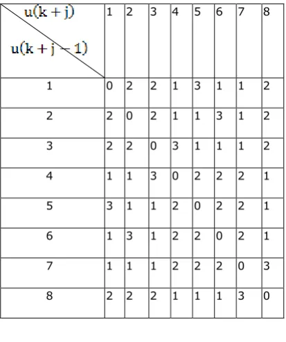
Pertaining MPC to LIM allows improvement in the performance when compared with previous approach, however, it is impossible to maintain the online optimization due to high computations. So it is impractical method. Maximum acceptable frequency may be exceeded. To overcome those ENMPC is suggested [10] shows eight combinations possible from three inverter switches. The control action is based on the dynamic behavior of the plant to be controlled. Hence, the control algorithm is designed depending on a plant’s model .Each combination is performed, and manipulated variables are noted. The variable that maximizes the tracking performance is selected i.e. formulated below.

(11)

The difference between speed reference trajectory and actual speed is termed as error. The iteration which has minimum difference will reduce the inverter switching frequency. Is the penalty term that is added in the objective function. Here, v is the predicted speed, w is speed reference, u is control signal, and Q and are Positive constants.

1 2 3 4 5 6 7 8

1 0 2 2 1 3 1 1 2

2 2 0 2 1 1 3 1 2

3 2 2 0 3 1 1 1 2

4 1 1 3 0 2 2 2 1

5 3 1 1 2 0 2 2 1

6 1 3 1 2 2 0 2 1

7 1 1 1 2 2 2 0 3

8 2 2 2 1 1 1 3 0

TABLE I

NUMBER OF CONTROL SWITCHES, WHERE INDICES 1, 2, …, 8

First column in the table indicates the number of

switching positions .

The constants should deceit more penalties in the starting time steps than later steps this is because to late the transition of switches.

(12)

(4)

Page 503

tracking errors. The modified objective function is

formulated.

(13)

Here, ˆE (k) is a prognosis of the sum of the tracking error E(k), where E(k) is determined as :

E(k + 1) = E(k) + K (w(k) − v(k))

(14)

v is the calculated speed, w is speed reference, and K is a gain. (14) Avoids the E from becoming too large with E(k+1) = E(k)and |E (k)| is greater than a specific bound.

Providing integral control is main criteria that our approach is focusing on. As already discussed about different ways of eliminating offset, refer [10], the concept of control limit [ <N] is employed to decrease the computational time and number of judging parameters. All other traditional approaches are not fit for this application. Where control signal is not continues valued signal and determines the technique of decreasing the number of optimization variables which is called blocking of the input parameters. =

Algorithm 1 Reducing the Computational Time: Pruning Rule

1) Initializing with =∞, (k) = 0 2) For i = 1 : s

3) Forj = 1 : N 4) Let

(k+ j )= (k+ j−1)+

Where is the incremental

Cost at time k+j due to the control signal (k + j − 1). 5) If (k + j) > break and go to step 2

End if End for 6) At j = N

If (k+ j )< , := (k + N) end if

End for

7) = the optimal value

To avoid testing each and every possible input combination over the control limit N, and to compute the optimal control signal sequence, a algorithm is proposed in the following, which is called incremental algorithm. is termed as candidate optimal control signal sequence i.e. an element in U×U×· · ·×U, those are Cartesian products and determined as S-1. In the above algorithm step 4, The raising cost is the prognosis cost at time step k+j due to the control signal (k+j-1).

+

Algorithm1 terminates the cost function sum for the control sequence earlier than anticipate, if the cost function at prognosis step j is greater than the current upper limit Jopt. This reduces calculation time. Main advantage of the MPC is its capability to manage the constraints. That is giving best control while keeping the given constraints within the limit. Confining current and flux constraints into proposed controller is easy. By adding the following line to the controller code.

1) If

in the same way, the switching combination that heads to breaking of the flux and current are neglected. The main objective is served here. i.e. the constraints are permitting the controller to track the speed reference. At the same time modifying the flux and the current within the constraints.

IV. SYSTEM CONFIGURATION

Block diagram of the LIM controlled with the suggested ENMPC controller, inverter and a flux estimator are shown in Fig 2. ENMPC controller input is w (speed reference), velocity of LIM v, primary currents and , and estimates of the secondary fluxes and .

,

(5)

[image:5.595.60.259.107.193.2]

Page 504

Fig.2. Block diagram of the LIM drive controlled with the

proposed ENMPC Controller.

Fuzzy Logic Controller

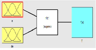
To make the proposed ENMPC controller even more efficient and robust against parameter variations, a Fuzzy Logic controller based on the Sugeno’s fuzzy interface model is designed for the existing controller. Various operating conditions of the LIM along with the proposed controller are given by fuzzy logic controller, the performance of the controller is tested.fig 3 shows the sugeno’s model employed for the controller.

Fig.3. Fuzzy Logic controller

Where e and de are the input variables to the nfc1 and the T is Output range [0,1] Ps(0.5), ze (0.25), ne(0) are output variables where each are different according the rule employed.

Fig.3 (A) Membership function of input 1

Input variable for the Membership function shown above is named as e. Range[-1.5 1.5] ze is of gauss mf type [0.3 0].

Fig.3(B)Membership function of input 2

Input variable for the Membership function shown above is named as de. Range [-150 150] ze is of gauss mf type [48.86 0.784].

Fig.3(c) Membership function of output

Fig 3(d) Sugeno’s Rule viewer

Rules used in FIS are as follows:

1) If (e = ne) and (de is ne) then (T is ne ) (1) 2) If (e = ne) and (de is ze) then (T is ze ) (1) 3) If (e = ne) and (de is ps) then (T is ps ) (1) 4) If (e = ze) and (de is ne) then (T is ne ) (1) 5) If (e = ze) and (de is ze) then (T is ze ) (1) 6) If (e = ze) and (de is ps) then (T is ps ) (1) 7) If (e = ps) and (de is ne) then (T is ne ) (1) 8) If (e = ps) and (de is ze) then (T is ze ) (1) 9) If (e = ps) and (de is ps) then (T is ps ) (1)

SIMULATION RESULTS AND DISCUSSION

[image:5.595.339.524.133.236.2] [image:5.595.347.521.284.370.2] [image:5.595.78.246.435.523.2] [image:5.595.70.252.619.713.2]

(6)

Page 505

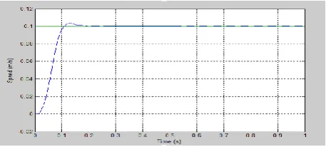
(Test 1) ENMPC Response and speed reference:

[image:6.595.315.552.157.248.2]

The LIM starts at time t=0 and continues to accelerate up to certain speed for instance we take that as 2m/s. when controller is replaced with DTC the control signal starts from t=0 and to attain the speed of 2m/s and to achieve steady state it took 0.1sec. When our new controller is employed the control signal takes only 0.01sec. to achieve the steady state, To track the speed reference PI controller is used, and the motor to reach the speed of 2m/s the time is assumed as 0.2s. the reason is the motor is small in Wight and has mechanical time constant of 0.007s.

Fig. 4 ENMPC Response and speed reference 3 phase, Y-connected, eight-pole, 3 kW, 60 Hz, 180 V, 14.2 A.

(Test 2) ENMPC Response with respect to Load

change:

[image:6.595.44.279.269.366.2]

The time differences between previous approach and ENMPC is same where to reach the steady state value under normal load, and when load disturbance occurs ENMPC recovers the control signal quickly and holds good performance. At time t=0.5s due to load change a small dip is occurred in speed reference but the controller is capable of restoring the signal very quickly than any other controller.

Fig.5. ENMPC Response with respect to Load change.

(Test 3) ENMPC Response against Ripples at low

Speed

LIM running at low speed is considered and when it is subjected to load disturbances the controller performance is examined and results shown,

that it is very quick in response. The ripples at low speed are difficult to control which was proved in DTC. ENMPC response curve shows it is capable of reducing ripples in 0.01sec and at 0.1sec ripples reduced significantly.

Fig.6. ENMPC Response against load change at low Speed.

[image:6.595.318.548.311.418.2]

ENMPC is more robust against the parameter

changes

Fig.6.a. ENMPC robust against the parameter changes.

Parameters and Data of the LIM

Rs (Ω)

5.3685

Pole pitch, h (m)

0.027

Rr (Ω)

3.5315

Total mass of the mover, M (kg).

2.78

Ls (H)

0.02846

Viscous friction and iron-loss coefficient ,D

(kg/s)

36.0455

Lr (H)

0.02846

Force constant, (N/wb

.A) 592

Lm (H)

0.02419

Rated secondary flux, (wb)

[image:6.595.47.276.548.651.2]

(7)

Page 506

(Test 4)Secondary flux and primary currents are

within the constraints.

The LIM is now run with low speed to check the controller performance. Such a low speed the electromagnetic force and three phase primary current responses were spotted in the fig7. It is obviously more challenging to track the results, where the load change is same and controller parameters are also same as previous case. At low speed worst case of torque and currents occurs, the bottom two plots shows what exactly happens when load changes. The three phase primary currents iabc and electromagnetic force have significantly less ripples when compared to previous approaches. The ENMPC controller responded quickly, even at low speed and shown good performance.

Fig.7. primary currents and Secondary flux are within the constraints

CONCLUSION

(8)

Page 507

REFERENCES

[1] G. Bucci, S. Meo, A. Ometto, and M. Scarano, “The control of LIM by a generalization of standard vector techniques,” in Proc. IEEE Ind.Elect. Control Instrum. Conf., Sep. 1994, pp. 623–626.

[2] I. Takahashi and Y. Ide, “Decoupling control of thrust and attractive force of a LIM using a space vector control inverter,” IEEE Trans. Ind.Appl., vol. 29, no. 1, pp. 161–167, Jan.–Feb. 1993.

[3] R. Rinkeviˇcien˙e and A. Smilgeviˇcius, “Linear induction motor at present time,” Electron. Electr. Eng. Technol., vol. 6, no. 78, pp. 3–8, 2007.

[4] G. H. Abdou and S. A. Sherif, “Theoritical and experimental design of LIM in automated manufacturing systems,” IEEE Trans. Ind. Appl., vol. 27, no. 2, pp. 286–293, Mar.–Apr. 1991.

[5] A. Gastli, “Asymmetrical constants and effect of joints in the secondary conductors of a linear induction motor,”

IEEE Trans. Energy Convers., vol. 15, no. 3, pp. 251–256, Sep. 2000.

[6] I. Takahashi and T. Noguchi, “A new quick response and high efficiency control strategy for the induction motor,” IEEE Trans. Ind. Appl., vol. 22, no. 2, pp. 820–827, Sep.–Oct. 1986.

[7] T. Geyer, G. Papafotiou, and M. Morari, “Model predictive direct torque control—part I: Concept, algorithm and analysis,” IEEE Trans. Ind.Electron., vol. 56, no. 6, pp. 1894–1905, Jun. 2009.

[8] P. Cortes, M. P. Kazmierkowski, R. M. Kennel, D. E. Quevedo, and J. Rodriguez, “Predictive control in power electronics and drives,” IEEE Trans. Ind. Electron., vol. 55, no. 12, pp. 4312–4324, Dec.

2008.

[9] D. Q. Mayne, J. B. Rawlings, C. V. Rao, and P. O. M. Scokaert, “Constrained model predictive control: Stability and optimality,” Automatica, vol. 36, no. 6, pp. 789–814, Jun. 2000.

[10] F.-J. Lin, H.-J. Shieh, K.-K. Shyu, and P.-K. Huang, “On-line gain tuning IP controller using real coded genetic algorithm,” Electr. Power Syst.Res., vol. 72, no. 2, pp. 157– 169, 2004.

BIOGRAPHIES

Y.VishnuVardhan Reddy currently

pursuing M-Tech in Control Systems at JNTUA College of Engineering and

Technology Anantapur, Andhra

Pradesh.His area of interest is ControlSystems.

Speed tracking of a Linear Induction Motor Along with Fuzzy Logic control Using Enumerative Nonlinear Model Predictive control

Page 500