Sample Based Visualization and Analysis of Binary Search in Worst Case Using Two Step Clustering and Curve Estimation Techniques on Personal Computer

(1)

Page 1508

Sample Based Visualization and Analysis of Binary Search in Worst

Case Using Two-Step Clustering and Curve Estimation Techniques on

Personal Computer

Dipankar Das

1,*

_{, Arnab Kole}

2

_{, Parichay Chakrabarti}

3

1

_{Assistant Professor, BCA(H), The Heritage Academy, Kolkata, West Bengal, India}

2

_{Assistant Professor, BCA(H), The Heritage Academy, Kolkata, West Bengal, India}

3

_{Assistant Professor, BCA(H), The Heritage Academy, Kolkata, West Bengal, India}

---*---Abstract –**

The objective of the present study is to

visualize and analyze the performance of binary search in worst case on a personal computer. We have collected the searching time of binary search in worst case for data size one thousand (1000) to fifty thousand (50000) with an interval of one thousand (1000) and for each data size one hundred thousand (100000) observations have been recorded. This data have been analyzed employing ‘Two – Step’ clustering algorithm using both Euclidean and Log–likelihood distance measure. The biggest cluster for each data size has been identified and the mean of those clusters have been calculated which gave us the mean searching time for each data size. Mann – Whitney U Test has been used to test the distribution of mean searching time for both the cases and curve estimation technique has been used to find the best fitted curves for the dataset (mean searching time versus data size).

Key Words:

Binary Search, Two – Step Clustering,

Euclidean distance measure, Log – likelihood distance

measure, Curve Estimation

1. INTRODUCTION

A binary search or half-interval search algorithm which can be classified as a dichotomic divide-and-conquer search algorithm finds the position of a target value within a sorted array [16]. In case of the worst case in binary search, the searched value is not present in the set [17][18][19].

By clustering we mean it is the task of grouping a set of objects in such a way that objects in the same group are more similar to each other than to those in other groups [20]. The cluster analysis or segmentation analysis or taxonomy analysis is an explorative analysis that tries to

identify structures within the data [21]. Two-step cluster analysis identifies the groupings by running pre-clustering first and then by hierarchical methods [21]. In the Two-step cluster analysis the ‘distance measure’ determines how the similarity between two clusters is computed [22]. There are two types of distance measure (i) Log-likelihood and (ii) Euclidean. The likelihood measure places a probability distribution on the variables. The Euclidean measure is the "straight line" distance between two clusters [22].

2. RELATED WORK

For binomial inputs, a statistical comparison between linear search and binary search had been done by Kumari, Tripathi, Pal & Chakraborty (2012) [1].

Sapinder, Ritu, Singh & Singh (2012) in their work had compared and contrasted various sorting and searching algorithms in terms of various Halstead metrices and had shown binary search gave more optimized result as compared to linear search [2].

A randomized searching algorithm had been proposed by Das & Khilar (2013) in their research work, the performance of which lies between binary search and linear search [3].

A comparative analysis of linear search, binary search and interpolation search had been done by Roy & Kundu (2014). The advantages of binary search with respect to linear search and interpolation search for a given problem had been shown by the researchers in their research article [4].

A modified binary search algorithm had been proposed by Chadha, Misal & Mokashi (2014) in their work [5].

(2)

Page 1509

The linear search and binary search had been analyzed

and compared on the basis of time complexity for a given set of data by Pathak (2015) [7].

Das, Kole, Mukhopadhyay & Chakrabarti (2015) had done a comparative analysis of the performance of binary search in the worst case on two personal computers. For doing the analysis, the researchers have collected the searching time from data size one thousand (1000) to fifty thousand (50000) with an interval of one thousand and for each data size they have noted the execution time ten thousand times for each of these personal computers. To avoid any variations in the execution time they have calculated the average searching time for each data size and had conducted their research using these average searching times. In their study, the researchers have observed that the behavior of both the computers are different but both of the datasets can be best explained by three (3) different types of curves namely compound, growth and exponential [8].

3. OBJECTIVES OF THE STUDY

1. To find out the mean searching time of binary search in the worst case for each data size using Two-Step Clustering algorithm using the distance measure as (a) Euclidean and (b) Log – Likelihood (for the personal computer under study).

2. To visualize both the mean searching times (i.e. Euclidean distance measure and Log – Likelihood distance measure) using interpolation lines (for the personal computer under study).

3. To find out whether the distribution of mean searching time for both the cases (i.e. Euclidean distance measure and Log – Likelihood distance measure) is same or not across the categories of distance measure i.e. Euclidean and Log – Likelihood (for the personal computer under study).

4. To identify a threshold value from where the distribution of the mean searching time is same across categories of distance measure (for the personal computer under study).

5. To find out the best curve(s) that can be fitted to the data points i.e. mean searching time (using both the Euclidean distance measure and Log – Likelihood distance measure) versus data size for (i) all the data sizes and (ii) from the threshold value if it can be identified as set in objective number four (for the personal computer under study).

6. To identify the mathematical equations of the best fitted curves and to give visualizations of these curves (for the personal computer under study).

4. RESEARCH METHODOLOGY

4.1 Steps

Step 1: Step 1 is sample dataset generation. Windows operating system and Java have been used for generating the dataset. For doing this study, we have noted the execution time (in Nano – seconds) of binary search in worst case from data size one thousand (1000) to fifty thousand (50000) with an interval of one thousand (1000) on a particular personal computer. For each data size (i.e. from 1000 to 50000 with an interval of 1000) we have noted the execution time one hundred thousand (100000) times.

Step 2: In this step we have used the Two-Step Clustering algorithm [9]. We have calculated the mean searching time for each data size (i.e. from 1000 to 50000 with an interval of 1000) using Two-Step Clustering algorithm. We have used the distance measure as (a) Euclidean and (b) Log – Likelihood. The clustering criterion is chosen as Schwarz's Bayesian Criterion (BIC). At first, we have identified the largest cluster for each data size using Euclidean distance measure and noted the mean value of that cluster. After that we have identified the largest cluster for each data size using Log – Likelihood distance measure and noted the mean value of that cluster.

Step 3: Using the interpolation line [10][15] we have graphically represented the mean searching times for both the cases (i.e. Euclidean distance measure and Log – Likelihood distance measure) considering data size as x – axis and mean searching time as y – axis.

Step 4: We have tested the distribution of mean searching time for both the cases (i.e. Euclidean distance measure and Log – Likelihood distance measure) using Mann-Whitney U Test. The decision rule has been considered as follows - if the ‘Asymptotic’ significance is less than .05 then the two groups are significantly different [11].

Step 5: In this step, by employing trial and error technique we have identified the threshold value from where the distribution of the mean searching time is same across categories of distance measure. In this step also, we have used Mann-Whitney U Test for testing the distribution of mean searching times keeping the decision rule same as step 4.

(3)

Page 1510

distance measure and Log – Likelihood distance measure)

versus data size based on the goodness of fit statistics e.g.

R square (decision rule: high value of R square i.e. close to 1), Adjusted R square (decision rule: high value of Adjusted R square i.e. close to 1), Root Mean Square Error (decision rule: low value of RMSE i.e. close to 0) [12]. The normal distribution of the residuals of the best identified models are tested using Shapiro – Wilk (SW) test [13][14]. If the significance of SW statistic is higher than .05 then it suggests that the assumption of normality of error distribution has been met [13][14]. In this study, we have used the following eleven (11) types of models for curve estimation – linear, quadratic, compound, growth, logarithmic, cubic, s, exponential, inverse, power and logistics.

In this study, to avoid any inconsistencies / variations (e.g. outliers) the researchers have used Two-Step Clustering algorithm to identify the largest cluster for each data size and calculated the mean value of that cluster for each data size.

4.2 Hardware used

Intel(R) Core(TM)2 Duo CPU, 2.93 GHz; 2 GB of RAM.

4.3 Software used

Windows XP Operating System (Windows XP Professional, Version 2002, and Service Pack 3), Java (NetBeans IDE 7.0; Java: 1.6.0_17) and SPSS 20.

5. DATA ANALYSIS & FINDINGS

5.1 Mean searching time using Two-Step

clustering algorithm

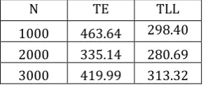
The mean searching time of binary search in worst case obtained using Two – Step Clustering algorithm for each data size (i.e. from 1000 to 50000 with an interval of 1000) is tabulated below (Table -1).

[image:3.595.35.184.693.757.2]

The Data size is denoted by N. The Mean Searching Time Using Distance Measure – Euclidean is denoted by TE and Mean Searching Time Using Distance Measure – Log Likelihood is denoted by TLL. The unit of time is ‘Nano seconds’.

Table -1: Data Size versus Mean Searching Time

N TE TLL

1000 463.64 298.40

2000 335.14 280.69

3000 419.99 313.32

4000 332.02 289.70

5000 322.54 301.66

6000 307.47 297.61

7000 312.81 295.65

8000 316.93 298.21

9000 321.80 307.73

10000 320.49 308.94

11000 324.40 307.30

12000 325.16 308.72

13000 316.54 307.89

14000 306.97 306.97

15000 311.85 307.12

16000 309.56 307.20

17000 316.79 316.63

18000 318.33 317.13

19000 321.20 317.10

20000 320.26 318.94

21000 332.69 330.04

22000 348.75 335.63

23000 337.40 337.11

24000 346.46 341.17

25000 357.65 346.03

26000 344.70 341.91

27000 355.97 349.34

28000 354.73 334.01

29000 367.58 362.11

30000 360.70 360.70

31000 369.77 367.21

32000 357.31 355.02

33000 359.65 358.39

34000 361.73 360.24

35000 359.46 357.35

36000 358.82 355.44

37000 358.69 357.43

38000 363.65 359.24

39000 355.85 355.64

40000 362.06 358.76

41000 358.33 357.87

42000 358.95 357.32

43000 358.28 356.98

44000 362.02 358.20

45000 361.34 359.53

46000 367.21 364.93

(4)

Page 1511

48000 358.26 354.00

49000 360.29 356.20

50000 365.46 364.63

5.2 Visualization of the mean searching times

using interpolation lines

Chart -1: TE versus N

Chart -2: TLL versus N

Findings: From the above table (Table -1) and the charts (Chart -1 & Chart -2) we observe that the minimum values of TE and TLL are 306.97 and 280.69 respectively, the maximum values of TE and TLL are 463.64 and 367.21 respectively and the range of TE and TLL are 156.67 and 86.52 respectively. From the charts (Chart -1 & Chart -2) we observe that both the interpolation lines appear to be different.

5.3 Testing the distribution of mean searching

times using Mann-Whitney U Test

The output of Mann – Whitney U test is given below (Fig - 1, 2 & 3).

Fig -1: Mean Rank of Mann – Whitney U Test for data size 1000 to 50000

Fig -2: Asymptotic Sig. (2 sided test) of Mann – Whitney U Test for data size 1000 to 50000

Fig -3: Result of Mann – Whitney U Test for data size 1000 to 50000

Findings: It has been observed from the above test that the distribution of mean searching time is not same across the categories of distance measure i.e. Euclidean and Log - Likelihood.

5.4 Identification of a threshold value from where

the distribution of the mean searching time is

same across categories of distance measure

[image:4.595.36.249.191.558.2] [image:4.595.308.511.240.350.2] [image:4.595.309.510.389.481.2]

(5)

[image:5.595.35.250.71.202.2]

Page 1512

Fig -4: Mean Rank of Mann – Whitney U Test for data size

4000 to 50000

Fig -5: Asymptotic Sig. (2 sided test) of Mann – Whitney U Test for data size 4000 to 50000

Fig -6: Result of Mann – Whitney U Test for data size 4000 to 50000

Findings: It has been observed from the above test that the distribution of mean searching time is same across the categories of distance measure i.e. Euclidean and Log - Likelihood. Therefore, we may select the data size 4000 as the threshold value from where the distribution of the mean searching time is same across categories of distance measure (for the personal computer under study).

5.5 Identification of the best curves that can be

fitted to the data points (mean searching time

versus

data size)

Case 1: TE versus N (data size 1000 to 50000)

Table -2: Goodness of fit statistics of TE versus N (data size 1000 to 50000)

Model

Name Square R Adjusted R

Square

RMSE

Linear .111 .092 27.004

Logarithmic .001 -.020 28.623

Inverse .185 .168 25.855

Quadratic .195 .161 25.964

Cubic .534 .503 19.978

Compound .150 .132 .073

Power .008 -.013 .079

S .138 .120 .073

Growth .150 .132 .073

Exponential .150 .132 .073

Logistic .033 .013 .329

Findings: From the above table (Table -2) we observe that none of the models are having high R square, high Adjusted R square values. The highest R square is .534 for Cubic model whose corresponding RMSE is 19.978. At the same time four models namely Compound, S, Growth and Exponential have low RMSE (.073) but their R square and Adjusted R square values are very low. Therefore in this case, amongst the eleven tried models, we do not find any curve which can be best fitted to the given dataset.

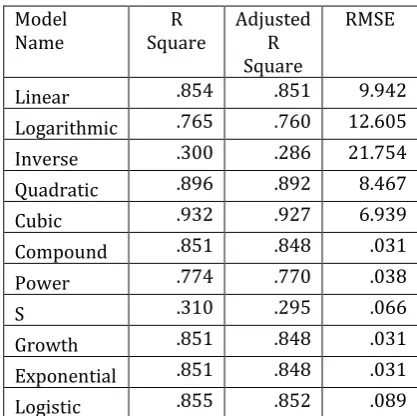
Case 2: TLL versus N (data size 1000 to 50000)

Table -3: Goodness of fit statistics of TLL versus N (data size 1000 to 50000)

Model

Square

RMSE

Linear .854 .851 9.942

Logarithmic .765 .760 12.605

Inverse .300 .286 21.754

Quadratic .896 .892 8.467

Cubic .932 .927 6.939

Compound .851 .848 .031

Power .774 .770 .038

S .310 .295 .066

Growth .851 .848 .031

[image:5.595.308.515.132.341.2] [image:5.595.36.242.239.351.2] [image:5.595.37.242.389.482.2] [image:5.595.306.515.526.734.2]

(6)

Page 1513

Findings: From the above table (Table -3) we observe that

Cubic model is having highest R square (.932) and highest Adjusted R square (.927) and the RMSE of Cubic model is 6.939. Therefore we are selecting this model as candidate model (candidate to be the best curve) in our study.

The test of normality of residuals of the candidate model is tabulated below (Table -4).

Table -4: Shapiro – Wilk (SW) test statistics of the candidate model for TLL versus N (data size 1000 to 50000)

Model

Name Shapiro-Wilk

Statistic df Sig.

Cubic .966 50 .160

Findings: The significance of SW statistics for the candidate model is higher than .05. Therefore, it suggests that the assumption of normality of error distribution has been met for the model.

From the findings of Table -3 and Table -4 we conclude that the Cubic curve may be best fitted to the data points i.e. TLL versus N (data size 1000 to 50000).

Case 3: TE versus N (data size 4000 to 50000)

Table -5: Goodness of fit statistics of TE versus N (data size 4000 to 50000)

Model

Square

RMSE

Linear .744 .739 10.552

Logarithmic .686 .679 11.691

Inverse .430 .418 15.747

Quadratic .770 .759 10.123

Cubic .851 .841 8.238

Compound .740 .734 .031

Power .683 .676 .035

S .428 .415 .047

Growth .740 .734 .031

Logistic .748 .742 .096

Findings: From the above table (Table -5) we observe that Cubic model is having highest R square (.851) and highest Adjusted R square (.841) and the RMSE of Cubic model is 8.238. Therefore we are selecting this model as candidate model (candidate to be the best curve) in our study.

The test of normality of residuals of the candidate model is tabulated below (Table -6).

Table -6: Shapiro – Wilk (SW) test statistics of the candidate model for TE versus N (data size 4000 to 50000)

Model

Name Shapiro-Wilk

Statistic df Sig.

Cubic .967 47 .206

From the findings of Table -5 and Table -6 we conclude that the Cubic curve may be best fitted to the data points i.e. TE versus N (data size 4000 to 50000).

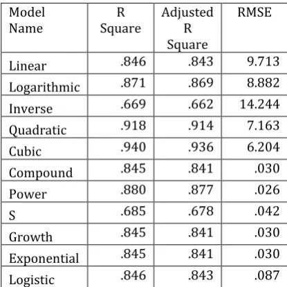
Case 4: TLL versus N (data size 4000 to 50000)

Table -7: Goodness of fit statistics of TLL versus N (data size 4000 to 50000)

Model

Square

RMSE

Linear .846 .843 9.713

Logarithmic .871 .869 8.882

Inverse .669 .662 14.244

Quadratic .918 .914 7.163

Cubic .940 .936 6.204

Compound .845 .841 .030

Power .880 .877 .026

S .685 .678 .042

Growth .845 .841 .030

Logistic .846 .843 .087

Findings: From the above table (Table -7) we observe that Cubic model is having highest R square (.940) and highest Adjusted R square (.936) and the RMSE of Cubic model is 6.204. Therefore we are selecting this model as candidate model (candidate to be the best curve) in our study.

[image:6.595.308.516.180.231.2] [image:6.595.36.244.251.301.2] [image:6.595.307.515.403.611.2] [image:6.595.35.245.474.683.2]

(7)

Page 1514

Table -8: Shapiro – Wilk (SW) test statistics of the

candidate model for TLL versus N (data size 4000 to 50000)

Model

Name Shapiro-Wilk

Statistic df Sig.

Cubic .970 47 .271

From the findings of Table -7 and Table -8 we conclude that the Cubic curve may be best fitted to the data points i.e. TLL versus N (data size 4000 to 50000).

5.6 Identification of the mathematical equations

of the best curves and visualization of these

curves

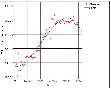
For case 2 i.e. TLL versus N (data size 1000 to 50000) Cubic curve has been identified as the best curve. The mathematical equation of the cubic curve is given below:

TLL = (-0.000146)*N + 1.279E-007*N^2 + (-2.040E-012)*N^3 + 294.559

The plot of the above model is given below (Chart -3).

Chart -3: Cubic curve of TLL versus N (data size 1000 to 50000)

For case 3 i.e. TE versus N (data size 4000 to 50000) Cubic curve has been identified as the best curve. The mathematical equation of the cubic curve is given below:

TE = (-0.003)*N + 2.211E-007*N^2 + (-2.974E-012)*N^3 + 329.228

Chart -4: Cubic curve of TE versus N (data size 4000 to 50000)

For case 4 i.e. TLL versus N (data size 4000 to 50000) Cubic curve has been identified as the best curve. The mathematical equation of the cubic curve is given below:

TLL = (0.000382)*N + 1.087E-007*N^2 + (-1.830E-012)*N^3 + 290.372

Chart -5: Cubic curve of TLL versus N (data size 4000 to 50000)

6. LIMITATIONS & FUTURE SCOPE

[image:7.595.37.251.465.634.2]

(8)

Page 1515

(BIC). Using this clustering algorithm with other criterion

may give us either same or different results, uncovering that will certainly be our future scope. Only eleven (11) models have been tried for curve fitting in this paper by the researchers. Using other models may unearth better fit for the datasets. At careful observation of Chart -1 and Chart -2 we notice that from data size 1000 to 4000 the interpolation lines show a ‘High – Low – High – Low’ shapes in both the cases. Therefore, taking more number of data points within this range i.e. 1000 to 4000 by decreasing the interval may help us to explain this behavior in future.

7. CONCLUSIONS

From this paper, we can conclude that for the personal computer under study, the distribution of mean searching time is not same across the categories of distance measure i.e. Euclidean and Log – Likelihood for the data size one thousand (1000) to fifty thousand (50000). The study identifies the data size four thousand (4000) as the threshold value from where the distribution of mean searching time is same across the categories of distance measure. In the present work, we cannot identify any curve which can be best fitted to the dataset of TE versus N for data size 1000 to 50000. The present study also shows that the cubic curve is the best fit for (i) TLL versus N (data size 1000 to 50000), (ii) TE versus N (data size 4000 to 50000) and (iii) TLL versus N (data size 4000 to 50000). In this paper, we have tried to analyze the performance of the binary search in worst case on a particular personal computer in a subtle way. However, overcoming the limitations as given in the section 6 will certainly give us more insights into the performance of binary search on personal computers which will undoubtedly be our future venture.

REFERENCES

[1] Kumari, A., Tripathi, R., Pal, M., & Chakraborty, S. (2012). Linear Search Versus Binary Search: A Statistical Comparison For Binomial Inputs.

International Journal of Computer Science,

Engineering and Applications (IJCSEA), 2(2). Retrieved

October 10, 2015, from

http://www.airccse.org/journal/ijcsea/papers/2212 ijcsea03

[2] Sapinder, Ritu, Singh, A., & Singh, H.L. (2012). Analysis of Linear and Binary Search Algorithms. International Journal of Computers & Distributed Systems, 1(1).

[3] Das, P., & Khilar, P. M. (2013). A Randomized Searching Algorithm and its Performance analysis with Binary Search and Linear Search Algorithms. International Journal of Computer Science &

Applications (TIJCSA), 1(11). Retrieved October 10,

2015, from

http://citeseerx.ist.psu.edu/viewdoc/download?doi= 10.1.1.300.7058&rep=rep1&type=pdf

[4] Roy, D., & Kundu, A. (2014). A Comparative Analysis of Three Different Types of Searching Algorithms in Data Structure. International Journal of Advanced

Research in Computer and Communication

Engineering, 3(5). Retrieved October 10, 2015, from http://www.ijarcce.com/upload/2014/may/IJARCCE 6C%20a%20arnab%20A%20Comparative%20Analy sis%20of%20Three.pdf

[5] Chadha, A. R., Misal, R., & Mokashi, T. (2014). Modified Binary Search Algorithm. arXiv preprint arXiv:1406.1677.

[6] Parmar, V. P., & Kumbharana, C. (2015). Comparing Linear Search and Binary Search Algorithms to Search an Element from a Linear List Implemented through Static Array, Dynamic Array and Linked List. International Journal of Computer Applications, 121(3). Retrieved October 10, 2015, from http://search.proquest.com/openview/a9b016911b 033e1e8dd2ecd4e7398fdd/1?pq-origsite=gscholar [7] Pathak, A. (2015). Analysis and Comparative Study of

Searching Techniques. International Journal of

Engineering Sciences & Research Technology, 4(3),

235-237. Retrieved October 10, 2015, from http://www.ijesrt.com/issues pdf

file/Archives-2015/March-2015/33_ANALYSIS AND

COMPARATIVE STUDY OF SEARCHING

TECHNIQUES.pdf

[8] Das, D., Kole, A., Mukhopadhyay, S., & Chakrabarti, P. (2015). Empirical Analysis of Binary Search Worst Case on Two Personal Computers Using Curve Estimation Technique. International Journal of Engineering and Management Research, 5(5), 304 – 311. Retrieved November 10, 2015, from http://www.ijemr.net/DOC/EmpiricalAnalysisOfBina rySearchWorstCaseOnTwoPersonalComputersUsing CurveEstimationTechnique%28304-311%29.pdf [9] Conduct and Interpret a Cluster Analysis - Statistics

Solutions. (n.d.). Retrieved November 10, 2015, from http://www.statisticssolutions.com/cluster-analysis-2/

[10]Curve fitting. (n.d.). Retrieved November 12, 2015, from https://en.wikipedia.org/wiki/Curve_fitting [11]Cramming Sam’s Tips for Chapter 6: Non - parametric

models. (n.d.). Retrieved October 10, 2015, from https://edge.sagepub.com/system/files/Chapter6.pd f

[12]Evaluating Goodness of Fit. (n.d.). Retrieved October

10, 2015, from

http://in.mathworks.com/help/curvefit/evaluating-goodness-of-fit.html

(9)

Page 1516

International journal of scientific and engineering

research, 5(6), 1218-1226. Retrieved October 10,

2015, from

http://www.ijser.org/researchpaper%5CPerformanc e-Measurement-and-Management-Model-of-Data-Generation.pdf

[14]Testing for Normality using SPSS Statistics. (n.d.). Laerd statistics. Retrieved October 10, 2015, from https://statistics.laerd.com/spss-tutorials/testing-for-normality-using-spss-statistics.php

[15]Matlab Curve Fitting and Interpolation. (n.d.).

Retrieved November 12, 2015, from

http://ef.engr.utk.edu/ef230-2011-01/modules/matlab-curve-fitting/

[16]Binary search algorithm. (n.d.). Retrieved November

12, 2015, from

https://en.wikipedia.org/wiki/Binary_search_algorit hm

[17]1 Time Complexity of Binary Search in the Worst Case. (n.d.). Lecture. Retrieved October 3, 2015, from http://www.csd.uwo.ca/Courses/CS2210a/slides/bi nsearch.pdf

[18]Analysis of Binary Search. (n.d.). Retrieved October 1,

2015, from

http://www2.hawaii.edu/~janst/demos/s97/yongsi /analysis.html

[19]Rao, R. (n.d.). CSE 373 Lecture 4: Lists. Lecture.

Retrieved October 1, 2015, from

https://courses.cs.washington.edu/courses/cse373/ 01sp/Lect4.pdf

[20]Cluster analysis. (n.d.). Retrieved October 1, 2015, from https://en.wikipedia.org/wiki/Cluster_analysis [21]Conduct and Interpret a Cluster Analysis - Statistics

Solutions. (n.d.). Retrieved November 12, 2015, from http://www.statisticssolutions.com/cluster-analysis-2/

[22]IBM Knowledge Center. (n.d.). Retrieved November 7,

2015, from

http://www-01.ibm.com/support/knowledgecenter/SSLVMB_21. 0.0/com.ibm.spss.statistics.help/idh_twostep_main.ht m

BIOGRAPHIES

Dipankar Das is currently

working as an Assistant Professor

in The Heritage Academy,

Kolkata, India. His area of interest includes Data Analytics, Curve

Fitting and Experimental

Algorithmics etc.

Arnab Kole is currently working as an Assistant Professor in The Heritage Academy, Kolkata, India. His area of interest includes

Artificial Intelligence,

Computational Mathematics and Finite Automata etc.

Parichay Chakrabarti is currently working as an Assistant Professor

in The Heritage Academy,

Kolkata, India. His area of interest includes Green Computing, Web

Development and Image

Sample Based Visualization and Analysis of Binary Search in Worst Case Using Two Step Clustering and Curve Estimation Techniques on Personal Computer

Page 1508