Impact of the joint detection-estimation approach on
random effects group studies in fMRI
Solveig Badillo, Thomas Vincent, Philippe Ciuciu
To cite this version:
Solveig Badillo, Thomas Vincent, Philippe Ciuciu. Impact of the joint detection-estimation
approach on random effects group studies in fMRI. Pan X, Liebling M,. ISBI 2011 - IEEE
Computer Society International Symposium on Biomedical Imaging: From Nano to Macro,
Mar 2011, Chicago, United States. IEEE, pp.376-380, 2011,
<
10.1109/ISBI.2011.5872427
>
.
<
hal-00854626
>
HAL Id: hal-00854626
https://hal.inria.fr/hal-00854626
Submitted on 3 Sep 2013
HAL
is a multi-disciplinary open access
archive for the deposit and dissemination of
sci-entific research documents, whether they are
pub-lished or not.
The documents may come from
teaching and research institutions in France or
abroad, or from public or private research centers.
L’archive ouverte pluridisciplinaire
HAL, est
destin´
ee au d´
epˆ
ot et `
a la diffusion de documents
scientifiques de niveau recherche, publi´
es ou non,
´
emanant des ´
etablissements d’enseignement et de
recherche fran¸
cais ou ´
etrangers, des laboratoires
publics ou priv´
es.
IMPACT OF THE JOINT DETECTION-ESTIMATION APPROACH ON RANDOM EFFECTS
GROUP STUDIES IN FMRI
Solveig Badillo, Thomas Vincent and Philippe Ciuciu
CEA, Neurospin, Bât. 145 - Point Courrier 156
F-91191 Gif-sur-Yvette, cedex France
Email: [email protected]
ABSTRACT
Inter-subject analysis of functional Magnetic Resonance Imaging (fMRI) data relies on single intra-subject studies, which are usually conducted using a massively univari-ate approach. In this paper, we investigunivari-ate the impact of an improved intra-subject analysis on group studies. basi-cally thejoint detection-estimation(JDE) framework [?, 1, 2] where an explicit characterization of the Hemodynamic Re-sponse Function (HRF) is performed at a regional scale and a stimulus-specific adaptive spatial correlation model en-ables the detection of activation clusters at voxel level. For the group statistics, we conducted several Random effect analyses (RFX) which relied either on the General Linear Model (GLM), or on the JDE analyses, or even on an inter-mediate approach named Spatially Adaptive GLM (SAGLM). Our comparative study perfomed during a fast-event related paradigm involves 18 subjects and illustrates the region-specific differences between the GLM, SAGLM and JDE analyses in terms of statistical sensitivity. On different con-trasts of interest, spatial regularization is shown to have a beneficial impact on the statistical sensitivity. Also, by study-ing the spatial variability of the HRF, we demonstrate that the JDE framework provides more robust detection perfor-mance in cognitive regions due to the higher hemodynamic variability in these areas.
Index Terms— fMRI, group analysis, RFX, GLM, joint detection-estimation, hemodynamics, Bayesian inference.
1. INTRODUCTION
In fMRI studies, two strategies are available to improve the quality of the data (such as reducing distorsion artifacts and/or improving spatial and temporal resolution). The first approach(i)consists in developing advanced estimation tech-niques while the second one(ii)rests on improved acquisition setups at higher static magnetic fields or using parallel imag-ing. The analysis methods developed in(i) are both robust against noise and able to adapt properly to the underlying physiology, by modeling the spatio-temporal fluctuations of the observed BOLD (Blood Oxygen Level Dependent) signal.
In this respect, a Bayesian detection-estimation approach has been proposed in [?, 2]. This method jointly detects which parts of the brain are involved in a given task or stimulus and estimates the underlying dynamics of activations. Further extended in [1], Adaptive Spatial Mixture Models (ASMM) have been introduced to model spatial correlation of fMRI data instead of uniformly smoothing them.
A previous work [3] has assessed the improvement pro-vided by a supervised JDE approach where the maount of spatial correlation was set empirically compared to the clas-sical GLM-based framework using SPM51. The present pa-per generalizes this previous contribution [3] in the follow-ing directions: a) it studies the impact of automatic and spa-tially adaptive regularization and b) it enables the compari-son ofspatially unsupervised JDE framework [1] with both the GLM-based inference and and the SAGLM approach or theconstrainedJDE version in which the HRF is fixed to its canonical shape. Here, we show results for a large dataset acquired on a 32-channel head coil at a high (2x2 mm2) in-plane resolution. However, our global study investigated both issues(i)and(ii)by comparing the impact of using different spatial resolutions, acceleration factors and reconstruction al-gorithms in a parallel imaging context on group statistics.
This paper is structured as follows. For the sake of self-consistency, the classical fMRI analysis framework is sum-marized in Section 2. The JDE approach is presented in Sec-tion??. It relies on a prior parcellation of fMRI data, which derives from a clustering procedure that preserves connectiv-ity and functional homogeneconnectiv-ity. Then, at the parcel level the JDE framework allows us to specify and estimate a specific BOLD model. Section??is devoted to group studies in fMRI where the principles of random effect analysis are reminded. In Section??, results obtained at the group level using dif-ferent subject-level inferences are compared on two salient contrasts of interest of a quick fMRI mapping experiment. A special attention is paid to the HRF variability in the motor and parietal regions. Conclusions are drawn in Section??.
2. CLASSICAL WITHIN-SUBJECT ANALYSIS IN fMRI
2.1. Standard GLM-based approach
GLM-based methods correspond to hypothesis-driven ap-proaches that postulate a canonical shape for the HRFhcand enable voxelwise inference. In its simplest form, the model of the BOLD response is spatially invariant and remains con-stant across the brain. Hence, each regressor in thedesign
matrixX is built as the convolution ofhcwith the stimula-tion signal xm associated with the mth stimulus type. The
GLM therefore reads:
[y1, . . . ,yJ] =X[β1, . . . , βJ] + [b1, . . . ,bJ] (1) whereyj is the fMRI time series measured in voxel Vj at times(tn)n=1:N andβj ∈ RM defines the vector of BOLD effects inVj for all stimulus typem = 1 : M. Noisebj is usually modelled as a first-order autoregressive (i.e.,AR(1)) process in order to account for the spatially-varying temporal correlation of fMRI data [4]:bj,tn=ρjbj,tn−1+εj,tn, ∀j, t,
withεj∼ N(0N, σε2jIN), where0Nis a null vector of length N, andIN stands for the identity matrix of sizeN. Then, the BOLD magnitudes estimatesβbj are computed in the maxi-mum likelihood sense as follows:βbj = arg minβ∈RMkyj−
Xβjk2bσ−2
εjΛjb , where σb −2
εj Λbj defines the inverse of the
esti-mated autocorrelation matrix ofbj; see [5] for details about the identification of the noise. Later, extensions that incorpo-rate prior information on the BOLD effects(βj)j=1:J have been developed in the Bayesian framework [?, 6]. In such cases, vectors(βbj)j=1:Jare computed using more computa-tionally demanding strategies. However, all these contribu-tions consider a unique and global model HRF model while intra-individual differences in its characteristics have been ex-hibited between cortical areas [7].
2.2. Flexible GLM models
Although smaller than inter-individual fluctuations, the intra-subject regional variability of the HRF is large enough to be treated with care. GLM can actually be refined to account for variations of the canonical HRFhcat the voxel level through additional regressors: hc can be supplemented with its first and second derivatives ([hc|h′c|h
′′
c]) to model eg. differ-ences in time-to-peak. Although powerful and elegant, flexi-bility is achievable at the expense of fewer effective degrees of freedom and decreased sensitivity in any subsequent sta-tistical test. In this case, the BOLD effect is modelled using several regressors (βmj ∈RP) and the Student-t statistic can no longer be used to infer on differencesβmj −βnj between themth
andnth
stimulus types. Rather, anunsigned Fisher statistic has to be computed, making direct interpretation of activation maps more difficult.
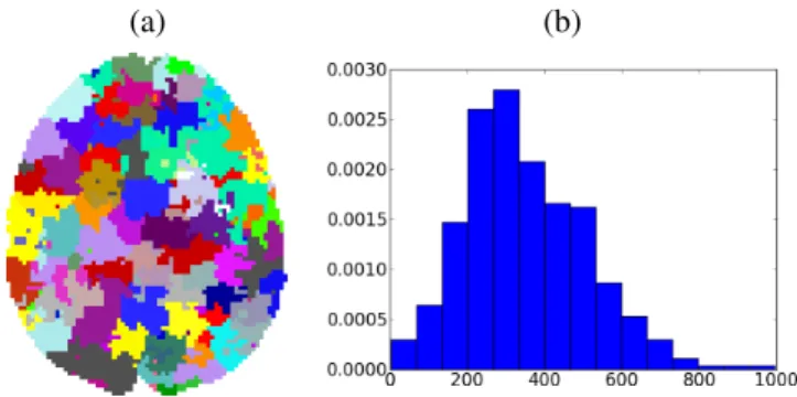
(a) (b)
Fig. 1. (a) Axial view of a color-coded multi-subject parcel-lation. (b): normalized histogram of parcel sizes for the same parcellation.
3. BEYOND THE GLM TO WITHIN-SUBJECT ANALYSIS IN fMRI
3.1. Multi-subject parcellation
Here, we claim the necessity of a spatially varying HRF model to keep asingleregressor per condition, and thus en-able the direct statistical comparison (βbm
j −βbjn). The JDE framework proposed in [?, 1, 2] enables the introduction of a spatially adaptive GLM, where a local estimation of h
is performed. To conduct the analysis efficiently, HRF es-timation is performed at a regional coarser scale than the voxel level. To define this scale, the functional brain mask is divided inΓfunctionally homogeneousparcelsusing a par-cellation technique proposed in [8]. This algorithm relies on the minimization of a compound criterion reflecting both the spatial and functional structures and hence the topology of the dataset. The spatial similarity measure favours the closeness in the Talairach coordinates system. The functional part of this criterion is computed on parameters that characterize the functional properties of the voxels (eg, fMRI time series).
The number of parcelsΓ is set by hand. The larger the number of parcels, the stronger the degree of within-parcel homogeneity but potentially the lower the signal-to-noise ratio (SNR). To objectively choose an adequate number of parcels, theoretic information criteria have been investigated in [?]: converging evidence forΓ ≈500has been shown for a whole brain analysis leading to typical parcel sizes around a few hundreds voxels. Fig. ?? illustrates the group-level parcellation and the corresponding histogram of parcel sizes.
3.2. Parcel-based modeling of the BOLD signal
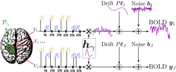
Here, we use the parcel-based model of the BOLD signal in-troduced in [1, 2]. LetPγ = (Vj)j=1:Jbe the current parcel. As shown in Fig. 1, this means that the HRF shapehγis con-stant within a parcel but that the magnitude of activationβm j may vary in space and across stimulus types:
yj= M X m=1 βm j Xmhγ+P ℓj+bj, ∀j, Vj ∈ Pγ. (2)
Fig. 2. Regional model of the BOLD signal in the JDE frame-work. The neural response levelsam
j match with the BOLD effectsβm
j .
Xmdenotes theN×(D+ 1)binary matrix that codes the onsets of themth stimulus. Vectorh
γ ∈ RD+1 represents the unknown HRF shape in Pγ. The term P ℓj models a low-frequency trend to account for physiological artifacts and noisebj ∼N(0N, σ2εjΛ
−1
j )stands for the above mentioned AR(1) process.
3.3. Bayesian JDE inference
The HRF shapehγand the associated BOLD effects(βj)j=1:J are jointly estimated inPγ. Since no parametric model is con-sidered forhγ, a smoothness constraint on the second order derivative is introduced to regularize its estimation; see [2] for details. On the other hand, our approach also aims at
detectingwhich voxels inPγ elicit activations in response to stimulation. To this end, prior mixture models are introduced on (βm)m=1:M to segregate activating and non-activating voxels in a stimulus-specific manner i.e., for eachm. In [1], it has been shown that ASMM allow us to recover clusters of activation instead of isolated spots using hidden Markov mod-els on voxel states. The level of spatial correlation in these models is automatically tuned from the data and may vary accross brain regions and between conditions since both the contrast-to-noise ratio the spatial activation pattern fluctuate accross stimulus types.
As our approach stands in the Bayesian framework, other priors are formulated upon every other sought object in Eq. (2); see [1] for details. Finally, inference is based upon the full posterior distribution p(h,(βj),(ℓj),Θ|y), which is sampled using a hybrid Metropolis-Gibbs sam-pling scheme [1]. Posterior mean (PM) estimates are there-fore computed from these samples according to: bxPM = PL1
k=L0x
(k)/L,
∀x ∈ h,(βj),Θ where L = L1 −
L0+ 1and L0 stands for the length of the burn-in period. Note that this estimation process has to be repeated over each parcel of each subject’s brain. Since the fMRI data are considered spatially independent across parcels, parallel im-plementation enables fast computation: whole brain analysis is achievable in about 60 mn forN = 128andΓ = 500. Compared to [3] which resorted to supervised estimation, the use of ASMM does not significantly increase the
com-putation load since a specific min-max procedure has been developed to approximate parcel-dependent partition func-tions of MRFs [1]. In this paper, we also investigate the use of ASMM combined with the GLM framework by setting the HRF shape to the canonical form in the JDE formalism. This approach is referenced SAGLM in what follows.
4. CLASSICAL PARAMETRIC POPULATION-BASED INFERENCE
Assume thatS subjects are selected randomly in a popula-tion of interest and involved in the same fMRI experiment. As shown in previous sections, the two types of within-subject analyses produce BOLD effect estimates βbj,s, in one particular voxel Vj of the standardized space (usually, the MNI/Talairach space) and for each subjects. Compar-ison between experimental conditions is usually addressed through contrast definition. Here, we restrict ourselves to scalar contrasts. Hence, we focus on signed differences
b dm−n
j,s = βbj,sm −βbj,sn of the BOLD effect relative to them
th
andnthstimulus types. For the sake of notational simplicity,
we drop subscriptjand superscriptm−n.
While the estimated differencedbs generally differs from the true but unobserved effect ds, assume for now perfect intra-subject estimation so thatdbs = dsfor s = 1 :S. We thus are given a sample (d1, , . . . , dS)drawn from an un-known probability density function f(d) that describes the distribution of the effects in the population. Here, we are concerned with inferences about a location parameter (mean, median, mode, ...). Assume for instance we wish to test the null hypothesis that the population mean is negative: H0 :
µG=
R
d f(d)dd≤0whereGstands for the group. To that end, we may use the classical one-samplettest. We start with computing thetstatistic:
t= µˆG ˆ σG/√S , with ˆµG= P sds S , σˆ 2 G= P s(ds−µˆG)2 S−1 .
Next, we rejectH0, hence accept the alternativeH1:µG >0, if the probability underH0of reaching the observedtvalue is lower than a given false positive rate. Under the assump-tion thatf(d)is gaussian, this probability is well-known to be obtained from the Student distribution with
5. EXPERIMENTAL RESULTS 5.1. Experimental protocol
fMRI data were recorded at 3 T (Siemens Trio) using a gradient-echo EPI sequence (TE=30ms/TR=2400ms/slice thickness=3mm/transversal orientation/FOV=192mm2) dur-ing a cognitive localizer experiment. The paradigm was a fast event-related design comprising sixty auditory, visual and motor stimuli, defined in ten experimental conditions (audi-tory and visual sentences, audi(audi-tory and visual calculations,
left/right auditory and visual clicks, horizontal and vertical checkerboards). For the considered dataset, the acquisition consisted of a single session of N = 128 scans lasting
TR= 2.4s each, yielding 3-D volumes with an anisotropic resolution of2×2×3mm3. A 32 channel volume coil was used to enable parallel imaging. The mSENSE parallel imag-ing reconstruction algorithm was applied with an acceleration factorR= 2for all the 18 subjects2.
5.2. Random effect (RFX) analyses
To enforce the coherence of our group level comparison with actual pipelines for fMRI data processing (SPM, FSL, BrainVISA-fMRI toolbox), the fMRI images that enter in GLM-based analysis were spatially filtered using isotropic Gaussian smoothing at FWHM=3mm. However, in the JDE formalism, we still consider unsmoothed but normalized fMRI data. The contrast images used for the two group analyses (based on intra-subjects analyses with SPM or JDE frameworks) remained alsounsmoothed.
Figs.??and??provide us with the group level Student-t maps for the three estimation procedures and two contratsts of interest. Fig.??focus on theLc. – Rc.contrast that highlights brain regions responding more to the left click than to the right click whatever the modality (auditory or visual). It is shown that the classical GLM-based, JDE-based and SAGLM-based inferences qualitatively yield almost the same results: a con-tralateral cluster in the motor cortex is found by all inference schemes. Due to spatial smoothing, GLM-based inference exhibits a larger cluster than alternative approaches but re-trieves a lower voxel-level maximum T-value value than the SAGLM-based inference as shown in Table 1. Also, for this motor contrast, we observe that the JDE framework provides the less sensitive results because the estimated HRF shape closely matches the canonical one in motor areas.
Fig.??presents the same comparison for the more cogni-tiveComputation – Sentences (C. – S.)contrast that elicits evoked brain activity in the fronto-parietal network. Here, the SAGLM-based inference provides larger activation cluster in the parietal and frontal lobes as expected [?]. This indicates the strong impact of spatially adaptive regularization. How-ever, the JDE framework gives the highest T-max peak value demonstrating that a better HRF modeling enhances the fit to fMRI data in higher cognitive regions. For thisC. – S.
contrast, the GLM-based inference appears to be the less sen-sitive both at the voxel and cluster levels: see Table 1 for de-tails. Besides, the GLM and SAGLM-based analyses found one cluster in the right prefrontal gyrus that was not recov-ered in [?], indicating the presence of false positives in this region.
These results are explained by the hemodynamic variabil-ity between the motor and parietal regions: HRF estimates
2One k-space line out of two was sampled along the phase encoding
di-rection.
(a) (b) (c)
Axial
Coronal
Sagittal
Fig. 3. Maximum Intensity Projection (MIP) of the RFX student-t maps for theLc. – Rc. contrast (thresholded at
P ≤0.001andK = 100for voxel-level and cluster-extent inferences, respectively). Neurological convention: left is left. Columns (a)-(b)-(c): results derived using the JDE, SPM, SAGLM analyses at the subject level, respectively.
(a) (b) (c)
Axial
Coronal
Sagittal
Fig. 4. MIP of the RFX student-t maps for theC. – S. con-trast. Same conventions as in Fig.??
(a) (b)
Time in s. Time in s.
Fig. 5. HRF estimates at the maximum intensity peak for all subjects. (a)-(b) correspond to the Lc. – Rc. andC. – S.
contrasts, respectively. Canonical HRF in black dotted line.
in the motor region have a shape closer to the canonical form (Fig. 4(a)) in contrast to their counterpart in the pari-etal region (Fig. 4(b)). Hence, there is a loss in statistical sensitivity when estimating the HRF shape in motor regions as reported on group studies in Fig.??. In more cognitive regions, HRF estimation is beneficial since group-level re-sults are more sensitive than those obtained considering a canonical HRF.
Table 1. Suprathreshold clusters summary for the t-statistic. Cluster size Voxel level Peak coords.
(voxels) Tmax x y z C. – S. JDE 514 10.77 −32 −54 45 SPM 617 8.7 −28 −66 48 SAGLM 780 10.59 −30 −56 45 Lc. – Rc. JDE 169 6.76 44 −16 48 SPM 454 10.12 36 −22 54 SAGLM 390 12.21 38 −22 57 6. CONCLUSION
In this paper, we extended previous results (see [3]) and showed that the type of intra-subject analysis impact group-level statistical analysis: Either the JDE formalism or the SAGLM framework provides more reliable RFX analysis results. In the parietal region, the JDE framework reported higher statistical peak values than SAGLM and GLM-based counterparts due to the high variability of the HRF in this area. In contrast, the SAGLM approach achieves the best compromise in the motor region because of spatially adaptive regularization. This seems to be due to a HRF shape closer to the canonical filter in this region. Future work will be devoted to a more extensive analysis of the between-regions hemodynamic variability.
7. REFERENCES
[1] T. Vincent, L. Risser, and P. Ciuciu, “Spatially adaptive mixture modeling for analysis of within-subject fMRI
time series,” IEEE Trans. Med. Imag., vol. 29, no. 4, pp. 1059–1074, Apr. 2010.
[2] S. Makni, J. Idier, T. Vincent, B. Thirion, G. Dehaene-Lambertz, and P. Ciuciu, “A fully Bayesian approach to the parcel-based detection-estimation of brain activity in fMRI,” Neuroimage, vol. 41, no. 3, pp. 941–969, July 2008.
[3] P. Ciuciu, T. Vincent, A.-L. Fouque, and A. Roche, “Im-proved fMRI group studies based on spatially varying non-parametric BOLD signal modeling,” in 5th Proc. IEEE ISBI, Paris, France, May 2008, pp. 1263–1266. [4] K.J. Worsley, C.H. Liao, J. Aston, V. Petre, G.H. Duncan,
F. Morales, and A.C. Evans, “A general statistical analy-sis for fMRI data,”Neuroimage, vol. 15, no. 1, pp. 1–15, Jan. 2002.
[5] W. D. Penny, S. Kiebel, and K. J. Friston, “Variational Bayesian inference for fMRI time series,” Neuroimage, vol. 19, no. 3, pp. 727–741, 2003.
[6] M. Woolrich, M. Jenkinson, J. Brady, and S. Smith, “Fully Bayesian spatio-temporal modelling of fMRI data,” IEEE Trans. Med. Imag., vol. 23, no. 2, pp. 213– 231, Feb. 2004.
[7] Daniel A. Handwerker, John M. Ollinger, , and Mark D’Esposito, “Variation of BOLD hemodynamic re-sponses across subjects and brain regions and their effects on statistical analyses,” Neuroimage, vol. 21, pp. 1639– 1651, 2004.
[8] B. Thirion, G. Flandin, P. Pinel, A. Roche, P. Ciuciu, and J.-B. Poline, “Dealing with the shortcomings of spatial normalization: Multi-subject parcellation of fMRI datasets,”Hum. Brain Mapp., vol. 27, no. 8, pp. 678–693, Aug. 2006.
[9] Phillip Good, Permutation, Parametric, and Bootstrap Tests of Hypotheses, Springer, 3rd edition edition, 2005.