Interval Simulation:
Raising the Level of Abstraction in Architectural Simulation
Davy Genbrugge
Stijn Eyerman
Lieven Eeckhout
Ghent University, Belgium
Abstract
Detailed architectural simulators suffer from a long de-velopment cycle and extremely long evaluation times. This longstanding problem is further exacerbated in the multi-core processor era. Existing solutions address the simula-tion problem by either sampling the simulated instrucsimula-tion stream or by mapping the simulation models on FPGAs; these approaches achieve substantial simulation speedups while simulating performance in a cycle-accurate manner.
This paper proposes interval simulation which takes a completely different approach: interval simulation raises the level of abstraction and replaces the core-level cycle-accurate simulation model by a mechanistic analytical model. The analytical model estimates core-level perfor-mance by analyzing intervals, or the timing between two miss events (branch mispredictions and TLB/cache misses); the miss events are determined through simulation of the memory hierarchy, cache coherence protocol, interconnec-tion network and branch predictor. By raising the level of abstraction, interval simulation reduces both development time and evaluation time.
Our experimental results using the SPEC CPU2000 and PARSEC benchmark suites and the M5 multi-core simula-tor, show good accuracy up to eight cores (average error of 4.6% and max error of 11% for the multi-threaded full-system workloads), while achieving a one order of magni-tude simulation speedup compared to cycle-accurate simu-lation. Moreover, interval simulation is easy to implement: our implementation of the mechanistic analytical model in-curs only one thousand lines of code. Its high accuracy, fast simulation speed and ease-of-use make interval simulation a useful complement to the architect’s toolbox for exploring system-level and high-level micro-architecture trade-offs.
1
Introduction
Architectural simulation is an invaluable tool in a com-puter architect’s toolbox for evaluating design trade-offs and novel research ideas. However, architectural simula-tion faces two major limitasimula-tions. First, it is extremely time-consuming: simulating an industry-standard benchmark for a single microprocessor design point easily takes a couple
days or weeks to run to completion, even on today’s fastest machines and simulators. Culling a large design space through architectural simulation of complete benchmark ex-ecutions thus simply is infeasible. While this is already true for single-core processor simulation, the current trend to-wards multi-core processors only exacerbates the problem. As the number of cores on a multi-core processor increases, simulation speed has become a major concern in computer architecture research and development. Second, developing an architectural simulator is tedious, costly and very time-consuming. Architectural simulators typically model the microprocessor in a cycle-accurate way, however, this level of detail is not always appropriate, nor is it called for. For example, early in the design process when the design space is being explored and the high-level microarchitecture is be-ing defined, too much detail only gets in the way. Or, when studying trade-offs in the memory hierarchy, cache coher-ence protocol or interconnection network of a multi-core processor, cycle-accurate core-level simulation may not be needed.
Researchers and computer designers are well aware of the multi-core simulation problem and have been propos-ing various fast simulation methodologies, such as sampled simulation [1, 8, 30, 32] and hardware-accelerated simula-tion using FPGAs [4, 26, 27, 31]. Although these method-ologies increase simulation speed and have their place in the architect’s toolbox, they model the multi-core processors at a high level of detail which impacts development time and which may not be needed for many practical research and development studies.
This paper takes a completely different approach and aims at raising the level of abstraction in architectural simu-lation. The key challenge in raising the level of abstraction in multi-core simulation is how to cope with the tight per-formance entanglement between co-executing threads. Co-executing threads affect each other’s performance through inter-thread synchronization and cache coherence, as well as through shared resources such as chip caches, on-chip interconnection network, off-on-chip bandwidth and main memory. Changes in the microarchitecture may change which parts of the threads execute together. This change, in its turn, may lead to different thread interleavings and dif-ferent conflict behavior in the shared resources, which may
lead to different relative progress rates for the co-executing threads. This tight performance entanglement between co-executing threads and the microarchitecture makes it hard to raise the level of abstraction in multi-core simulation.
This paper presents interval simulation, a novel, fast, accurate and easy-to-implement (multi-core) simulation paradigm. Interval simulation reduces both simulation time and simulator development complexity. Interval simula-tion raises the level of abstracsimula-tion in the individual cores compared to detailed simulation: a mechanistic analytical model [11] drives the timing simulation of the individual cores without the detailed tracking of individual instructions through the cores’ pipeline stages. The basis for the model is that miss events (branch mispredictions, cache and TLB misses) divide the smooth streaming of instructions through the pipeline into so called intervals. Branch predictor, mem-ory hierarchy, cache coherence and interconnection network simulators determine the miss events; the analytical model derives the timing for each interval. The cooperation be-tween the mechanistic analytical model and the miss event simulators enables the modeling of the tight performance entanglement between co-executing threads on multi-core processors.
Using both (multi-programmed) SPEC CPU2000 work-loads as well as the multi-threaded PARSEC benchmark suite, and the M5 full-system simulator, we evaluate ac-curacy and simulation speed compared to detailed cycle-level simulation. In terms of simulation speed, we attain a one order of magnitude improvement compared to detailed simulation. The error with respect to detailed simulation is 5.9% on average for the single-threaded SPEC CPU2000 benchmarks (max error of 16%); for the multi-threaded full-system PARSEC benchmarks, the average error is 4.6% across single-, dual-, quad- and eight-core processor config-urations (max error of 11%). In addition, we demonstrate that interval simulation yields similar performance trends and design decisions in practical research studies when trad-ing off the number of processor cores versus cache space versus memory bandwidth. Finally, the analytical core-level timing models simplify multi-core simulation development substantially. Our version of the interval simulator con-tains approximately 1K lines of C code to implement the analytical model. This is a dramatic reduction in complex-ity compared to the M5 out-of-order core simulator which comprises approximately 28K lines of code.
The goal of interval simulation is not to replace detailed cycle-by-cycle simulation. Instead, we view interval sim-ulation as a useful complement that offers high simsim-ulation speed and short simulator development time at slightly less accuracy. Interval simulation is envisioned as a fast sim-ulation technique to quickly explore the design space of multi-core processor architectures and make high-level mi-croarchitecture and system-level trade-offs; detailed cycle-accurate simulation can then be used to explore a region of interest.
The key contribution of this paper is to combine
core-branch misprediction
interval 2
long-latency load miss
t disp atchrate interval 3 interval 1 L1 I-cache miss
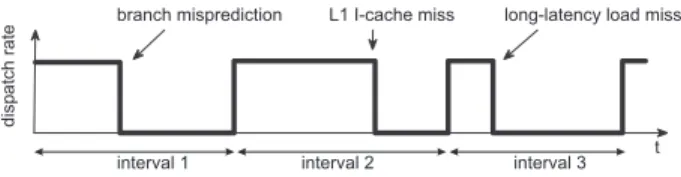
Figure 1. Interval analysis analyzes perfor-mance on an interval basis determined by disruptive miss events.
level analytical models with detailed simulation to accel-erate multi-core simulation. The challenge for doing so is to predict the timing for each individual instruction, not just average performance across all instructions as is done in an-alytical modeling [11] — estimating the timing per individ-ual instruction is required in order to accurately model syn-chronization, cache coherence, conflict behavior in shared resources, etc. Besides this major contribution, the paper also contributes to interval modeling in a number of sig-nificant ways: (i) it models overlapping miss events (e.g., I-cache misses and branch mispredictions overlapped by long-latency loads) — a second-order effect — prior work on the other hand focused on first-order effects (isolated miss events and overlapping long-latency loads) and did not model overlap effects between I-cache misses and branch mispredictions versus long-latency load misses; (ii) it mod-els serializing instructions and runs full-system code; (iii) it proposes the ‘old window approach’ to estimate the branch resolution time, window drain time and effective dispatch rate during simulation — prior work estimates the criti-cal path length through an offline profiling step; and (iv) it models multi-threaded execution including inter-thread synchronization and cache coherence.
2
Interval Analysis
Interval simulation builds on a recently developed mech-anistic analytical performance model, interval analysis [11], which we briefly revisit here. With interval analysis, execu-tion time is partiexecu-tioned into discrete intervals by disruptive miss events such as cache misses, TLB misses and branch mispredictions. The basis for the model is that an out-of-order processor is designed to smoothly stream instructions through its various pipelines and functional units. Under optimal conditions (no miss events), the processor sustains a level of performance more-or-less equal to its pipeline front-end dispatch width — we refer to dispatch as the point of entering the instructions from the front-end pipeline into the reorder buffer and issue queues.
The interval behavior is illustrated in Figure 1, which shows the number of dispatched instructions on the vertical axis versus time on the horizontal axis. By dividing exe-cution time into intervals, one can analyze the performance behavior of the intervals individually. In particular, one can, based on the type of interval (the miss event that
termi-nates it), describe and determine the performance penalty per miss event:
• For an I-cache miss (or I-TLB miss), the penalty equals
the miss delay, i.e., the time to access the next level in the memory hierarchy.
• For a branch misprediction, the penalty equals the time
between the mispredicted branch being dispatched and new instructions along the correct control flow path be-ing dispatched. This penalty includes the branch reso-lution time plus the front-end pipeline depth.
• Upon a long-latency load miss, i.e., a last-level L2
D-cache load miss or a D-TLB load miss, the proces-sor back-end will stall because of the reorder buffer (ROB), issue queue, or rename registers getting ex-hausted. As a result, dispatch will stall. When the miss returns from memory, instructions at the ROB head will be committed, and new instructions will en-ter the ROB. The penalty for a long-latency D-cache miss thus equals the time between dispatch stalling upon a full ROB and the miss returning from ory. This penalty can be approximated by the mem-ory access latency. In case multiple independent long-latency load misses make it into the ROB simultane-ously, both will overlap their execution, thereby expos-ing memory-level parallelism (MLP) [5], provided that a sufficient number of outstanding long-latency loads are supported by the hardware. The penalty of multiple overlapping long-latency loads thus equals the penalty for an isolated long-latency load. In case of dependent long-latency loads, their penalties serialize.
• Chains of dependent instructions, L1 data cache misses
and long-latency functional unit instructions (divide, multiply, etc.), or store instructions, may cause a re-source (e.g., reorder buffer, issue queue, physical reg-ister file, write buffer, etc.) to fill up. A resource stall as a result of it may (eventually) stall dispatch. The penalty or the number of cycles where dispatch stalls due to a resource stall are attributed to the instruction at the ROB head, i.e., the instruction blocking commit and thereby stalling dispatch.
3
Multi-core Interval Simulation
3.1
Framework overview and basic idea
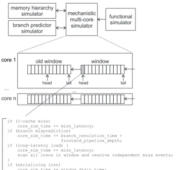
The multi-core interval simulation paradigm is drawn schematically in Figure 2. A functional simulator supplies instructions to the multi-core interval simulator which uses interval analysis for driving the timing of the individual cores. The miss events are handled by branch predictor and memory hierarchy simulators. The branch predictor simu-lator models the branch predictors in the individual cores and is invoked upon the execution of a branch instruction. The branch predictor simulator returns whether or not amechanistic multi-core simulator functional simulator memory hierarchy simulator branch predictor simulator window old window head
head tail tail
core 1 ... core 1 core n ... if (I-cache miss) core_sim_time += miss_latency; if (branch misprediction) core_sim_time += branch_resolution_time + frontend_pipeline_depth; if (long-latency load) { core_sim_time += miss_latency;
scan all insns in window and resolve independent miss events; }
if (serializing insn)
core_sim_time += window_drain_time;
Figure 2. Schematic view of the multi-core in-terval simulation framework.
branch is correctly predicted by the branch predictor. The memory hierarchy simulator models the entire memory hi-erarchy. This includes cache coherence, private (per-core) caches and TLBs, as well as the shared last-level caches, in-terconnection network, off-chip bandwidth and main mem-ory. The memory hierarchy simulator is invoked for each I-cache/TLB or D-cache/TLB access and returns the (miss) latency.
The multi-core interval simulator models the timing for the individual cores. The simulator maintains a ‘window’ of instructions for each simulated core, see Figure 2. This window of instructions corresponds to the reorder buffer of a superscalar out-of-order processor, and is used to deter-mine miss events that are overlapped by long-latency load misses. The functional simulator feeds instructions into this window at the window tail. Core-level progress (i.e., tim-ing simulation) is derived by considertim-ing the instruction at the window head. In case of an I-cache miss, we increase the core simulated time by the miss latency. In case of a branch misprediction, we increase the core simulated time by the branch resolution time plus the front-end pipeline depth. In case of a long-latency load (i.e., a last-level cache miss or cache coherence miss), we add the miss latency to the core simulated time, and we scan the window for in-dependent miss events (cache/TLB misses and branch mis-predictions) that are overlapped by the long-latency load — second-order effects. For a serializing instruction, we add the window drain time to the simulated core time. If none of the above cases applies, we dispatch instructions at the effective dispatch rate. Having determined the impact of the instruction at the window head on the core’s progress,
we remove the instruction from the window and feed it into the so called ‘old window’. The old window is used to de-rive the dependence chains of instructions and their impact on the branch resolution time, window drain time, and the effective dispatch rate in the absence of miss events, as we explain in detail in the following section.
3.2
Detailed algorithm
We refer to the high-level pseudocode given in Figure 3 for a more detailed description of multi-core interval simu-lation. The interval simulator iterates across all cores in the multi-core processor (line 2), and proceeds with the simu-lation as long as there are instructions to be simulated (line 3); if not, the simulator quits (line 71).
Multi-core simulated time versus per-core simulated time. The interval simulator simulates cycle per cycle, and keeps track of the multi-core simulated time as well as the per-core simulated time. The multi-core simulated time is incremented every cycle (line 74). The per-core simulated time is adjusted depending on the progress of the individual core, e.g., in case of a miss event, the per-core simulated time is augmented by the appropriate penalty. Only in case the per-core simulated time equals the multi-core simulated time, we need to simulate the cycle for the given core (line 6). In case the per-core simulated time is larger than the multi-core simulated time (which can happen because of miss events as we will describe next), we do not need to simulate the cycle for the given core. This could be viewed as event-driven simulation at the core level.
Instruction dispatch. As long as the core has dispatched fewer instructions than the effective dispatch rate in the given cycle, we continue simulating instructions (line 7). (We will describe how we compute the effective dispatch rate later.) The core-level simulation then considers the instruction at the window head (line 9) and determines its (potential) miss penalty (lines 11 to 59). We increment the number of dispatched instructions (line 62), remove the in-struction from the window, and insert the inin-struction in the old window (lines 64). We subsequently enter a new in-struction in the window at the tail pointer (line 65). Miss events. We access the I-cache and I-TLB (line 13). If this instruction is an I-cache miss or an I-TLB miss, we add the miss latency to the per-core simulated time (line 15). (We will explain the purpose of lines 12 and 16 later.)
The timing impact of a branch misprediction is fairly similar to an I-cache/TLB miss. We access the branch pre-dictor (line 22). If the branch is mispredicted (line 23), we add the branch penalty to the per-core simulated time. The branch penalty is computed as the sum of the branch resolution time and front-end pipeline depth (lines 24-25). We will explain how we estimate the branch resolution time
later; the front-end pipeline depth is a microarchitecture pa-rameter and is known.
For stores and non-overlapped loads (line 31), we access the memory hierarchy (i.e., caches, TLBs, and main mem-ory, including the cache coherence protocol) (line 32). In case of a long-latency load, we incur a miss penalty (i.e., the miss latency) which is added to the per-core simulated time (line 50).
Serializing instructions cause the core to drain the win-dow prior to their execution. Therefore, upon a serializing instruction, we increase the per-core simulated time with the penalty for emptying the old instruction window (lines 56–59).
Overlapping miss events. A long-latency load may hide latencies by other subsequent (independent) miss events — second-order effects. We therefore consider all instructions in the window from head to tail (line 35) upon a long-latency load and consider four cases (lines 35–49).
We access the I-cache and I-TLB for each instruction in the window past the long-latency load (line 36). We mark the instruction meaning that the I-cache/TLB access (a po-tential I-cache/TLB miss) is hidden by the long-latency load — this is done through theI overlappedvariable. This means that the I-cache/TLB access has occurred and should not incur any additional penalty when it appears at the win-dow head (line 12). In other words, the I-cache/TLB ac-cess/miss is hidden underneath the long-latency load.
We follow the same procedure for branches and loads if the branch/load is independent of the long-latency load (see lines 38–41 and 43–45, respectively). Independence means that there are no direct or indirect dependences (through registers or memory) between the branch/load and the long-latency load, and there appears no memory barrier between the two loads in the dynamic instruction stream. A branch or load that depends on a long-latency load serializes with the long-latency load and therefore does not get executed underneath the long-latency load.
In case we reach a serializing instruction while scanning the window upon a long-latency load, we break out of the loop and stop scanning the window (line 47). The serializ-ing instruction causes the window to be drained.
Branch resolution time, window drain time and effec-tive dispatch rate. An important component in interval simulation is to estimate the critical path length in the old window. The critical path length is used for computing (i) the branch resolution time, (ii) the window drain time upon a serializing instruction, and (iii) the effective dispatch rate. For computing the critical path length, we consider a data flow model that computes the earliest possible issue time for each instruction in the old window given its dependences and execution latency. This is done as follows. For each in-struction in the old window, we keep track of its execution latency (including the L1 D-cache miss latency), its issue
1: while (1) {
2: | for (i = 0; i < num_cores; i++) {
3: | | if (there are more insns to be simulated) { 4: | | |
5: | | | insns_dispatched = 0;
6: | | | while ((core_sim_time [i] == multi_core_sim_time) && 7: | | | | (insns_dispatched < eff_dispatch_rate(i)) { 8: | | | |
9: | | | | consider insn at window head; 10: | | | |
11: | | | | /* handle I-cache and I-TLB */ 12: | | | | if (!I_overlapped) {
13: | | | | | miss_latency = Icache_and_ITLB_access(); 14: | | | | | if (Icache_or_ITLB_miss) {
15: | | | | | core_sim_time [i] += miss_latency; 16: | | | | | empty_old_window();
17: | | | | | } 18: | | | | } 19: | | | |
20: | | | | /* handle branch prediction */ 21: | | | | if (branch && !br_overlapped) { 22: | | | | | branch_predictor_access(); 23: | | | | | if (branch_misprediction) {
24: | | | | | core_sim_time [i] += branch_resolution_time() + 25: | | | | | frontend_pipeline_depth; 26: | | | | | empty_old_window();
27: | | | | | } 28: | | | | } 29: | | | |
30: | | | | /* handle loads and stores */
31: | | | | if (store || (load && !D_overlapped)) { 32: | | | | | miss_latency = Dcache_and_DTLB_access(); 33: | | | | |
34: | | | | | if (long_latency_load) {
35: | | | | | | for (all insns in window from head to tail) { 36: | | | | | | | I_overlapped = 1; I_cache_and_ITLB_access(); 37: | | | | | | |
38: | | | | | | | if (branch && independent of long-latency load) { 39: | | | | | | | br_overlapped = 1; branch_predictor_access(); 40: | | | | | | | if (branch_misprediction) break;
41: | | | | | | | } 42: | | | | | | |
43: | | | | | | | if (load && independent of long-latency load) { 44: | | | | | | | D_overlapped = 1; Dcache_and_DTLB_access(); 45: | | | | | | | }
46: | | | | | | |
47: | | | | | | | if (serializing instruction) break; 48: | | | | | | |
49: | | | | | | }
50: | | | | | | core_sim_time [i] += miss_latency; 51: | | | | | | empty_old_window();
52: | | | | | } 53: | | | | } 54: | | | |
55: | | | | /* handle serializing instructions */ 56: | | | | if (serializing instruction) {
57: | | | | core_sim_time [i] += empty_window_latency(); 58: | | | | empty_old_window(); 59: | | | | } 60: | | | | 61: | | | | /* dispatch insn */ 62: | | | | insns_dispatched++; 63: | | | | 64: | | | | advance_window_head_pointer_and_insert_insn_in_old_window(); 65: | | | | enter_new_insn_at_window_tail_pointer_and_advance_tail_pointer(); 66: | | | }
67: | | | if (core_sim_time [i] == multi_core_sim_time) 68: | | | core_sim_time [i]++; 69: | | } 70: | | else { 71: | | finish_simulation(); 72: | | } 73: | } 74: | multi_core_sim_time++; 75: }
time, and its output dependences, i.e., the register(s) that it writes or the cache line that it writes in case of a store. For each instruction that is inserted at the old window tail, we compute its issue time as the maximum issue time of the instructions that it depends upon plus the instruction’s exe-cution time. We also keep track of the old window’s ‘head time’ and ‘tail time’. The new tail time is computed as the maximum of the previous tail time and the issue time of the newly inserted instruction; similarly, the new head time is the maximum of the previous head time and the issue time of the removed instruction. We then approximate the length of the critical path in the old window as the tail time minus the head time. This is an approximation of the real critical path in the old window. However, computing the real crit-ical path would require walking the old window for every newly inserted instruction, which is time-consuming and which is why we use the above approximation. We found the approximation to be accurate for our purpose, as we will demonstrate in the evaluation section.
Once we have computed the critical path length, we can compute the maximum possible execution rate through the old window. Using Little’s Law, we compute the execu-tion rate as window size divided by the critical path length. This reflects the fact that the out-of-order processor cannot process instructions faster than dictated by the critical path length. The effective dispatch rate then equals the minimum of this execution rate and the designed dispatch width. The branch resolution time is computed as the longest chain of dependent instructions (including their execution latencies) leading to the mispredicted branch, starting from the head pointer in the old window. The window drain time is com-puted as the maximum of (i) the number of instructions in the old window divided by the processor’s dispatch width, and (ii) the length of the critical execution path in the old window.
Interval length effect. Interval length (the number of in-structions between two subsequent miss events) has a sig-nificant impact on overall performance. In particular for a mispredicted branch, a short interval implies a short de-pendence path to the branch (i.e., short branch resolution time); a long interval on the other hand implies a longer branch resolution time. A similar effect occurs for serializ-ing instructions: a serializserializ-ing instruction causes the instruc-tion window to be drained. Window drain time is correlated with the interval length prior to the serializing instruction, i.e., the completely filled window takes longer to drain than a partially filled window. In order to model the dependence of interval length on the branch resolution time and window drain time, we empty the old window upon a miss event (see lines 16, 26, 30 and 58).
Functional-first simulation. Our current implementation of interval simulation employs a functional-first simulation approach. This means that the functional simulator
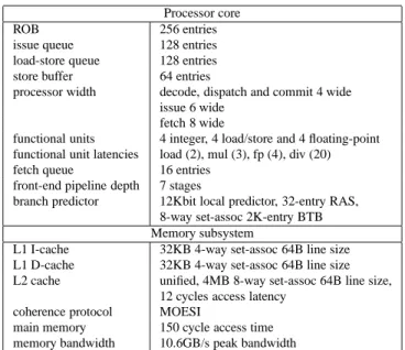
gener-Processor core
ROB 256 entries
issue queue 128 entries load-store queue 128 entries store buffer 64 entries
processor width decode, dispatch and commit 4 wide issue 6 wide
fetch 8 wide
functional units 4 integer, 4 load/store and 4 floating-point functional unit latencies load (2), mul (3), fp (4), div (20) fetch queue 16 entries
front-end pipeline depth 7 stages
branch predictor 12Kbit local predictor, 32-entry RAS, 8-way set-assoc 2K-entry BTB Memory subsystem
L1 I-cache 32KB 4-way set-assoc 64B line size L1 D-cache 32KB 4-way set-assoc 64B line size L2 cache unified, 4MB 8-way set-assoc 64B line size,
12 cycles access latency coherence protocol MOESI
main memory 150 cycle access time memory bandwidth 10.6GB/s peak bandwidth
Table 1. Baseline processor core model as-sumed in our experimental setup; simulated CMP architectures share the L2 cache.
ates a dynamic instruction stream, including user-level and system-level code, that is subsequently fed into the timing simulator. This implies that interval simulation does not simulate along mispredicted paths, and may lead to different thread interleavings than what may happen in real systems. A more accurate approach is to build a timing-directed sim-ulator in which the timing simsim-ulator directs the functional simulator along mispredicted paths and determines thread interleavings. This could be done by having the functional simulator operate at the window head rather than at the win-dow tail as is currently done. Unfortunately, timing-directed simulators are more difficult to develop because it requires checkpoint-and-rollback capability in the functional simu-lator and because it more tightly couples the functional sim-ulator with the timing simsim-ulator. In our current implemen-tation we opted for functional-first simulation because of its ease of development — this is a trade-off in development time, evaluation time and accuracy — and our evaluation shows good accuracy against the cycle-accurate M5 sim-ulator. We plan on implementing timing-directed interval simulation as part of our future work.
4
Experimental Setup
Benchmarks. We use two benchmark suites, namely SPEC CPU2000 and PARSEC. We use all of the SPEC CPU2000 benchmarks with the reference inputs in our ex-perimental setup. The binaries of the CPU2000 benchmarks were taken from the SimpleScalar website; these binaries were compiled for Alpha using aggressive compiler opti-mizations. We considered 100M simulation points as
deter-(a) Effective dispatch rate (b) I-cache/TLB 0.0 0.5 1.0 1.5 2.0 2.5 3.0 3.5 4.0 4.5 b z ip 2 c ra ft y e o n g a p g c c g z ip m c f p a rs e r p e rl b m k tw o lf v o rt e x v p r a m m p a p p lu a p s i a rt e q u a k e fa c e re c fm a 3 d g a lg e l lu c a s m e s a m g ri d s ix tr a c k s w im w u p w is IP C
detailed simulation interval simulation
0.0 0.5 1.0 1.5 2.0 2.5 3.0 3.5 4.0 4.5 b z ip 2 c ra ft y e o n g a p g c c g z ip m c f p a rs e r p e rl b m k tw o lf v o rt e x v p r a m m p a p p lu a p s i a rt e q u a k e fa c e re c fm a 3 d g a lg e l lu c a s m e s a m g ri d s ix tr a c k s w im w u p w is IP C
detailed simulation interval simulation
(c) Branch prediction (d) L2 cache
0.0 0.5 1.0 1.5 2.0 2.5 3.0 3.5 4.0 4.5 b z ip 2 c ra ft y e o n g a p g c c g z ip m c f p a rs e r p e rl b m k tw o lf v o rt e x v p r a m m p a p p lu a p s i a rt e q u a k e fa c e re c fm a 3 d g a lg e l lu c a s m e s a m g ri d s ix tr a c k s w im w u p w is IP C
detailed simulation interval simulation
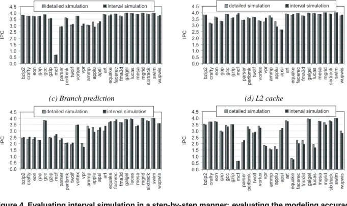
Figure 4. Evaluating interval simulation in a step-by-step manner: evaluating the modeling accuracy of the (a) effective dispatch rate, (b) I-cache/TLB, (c) branch prediction and (d) L2 cache.
mined by SimPoint [28] in all of our experiments in order to limit overall cycle-accurate simulation time — this is ex-actly the problem tackled by interval simulation. In addition to the single-threaded user-level SPEC CPU benchmarks, we also use the multi-threaded PARSEC benchmarks [2] which spend a substantial fraction of their execution time in system code. We use 9 of the 13 PARSEC benchmarks that run on our simulator with the small input set and run each benchmark to completion; the number of dynamically ex-ecuted instructions per benchmark varies between 500M to 13B instructions. The PARSEC benchmarks were compiled using the GNU C compiler for Alpha; we use aggressive optimization, including-O3, loop unrolling and software prefetching.
Simulator. We use the M5 simulator [3] in all of our experiments; M5 was previously validated against real Compaq Alpha machines. The SPEC CPU benchmarks are run in user-level simulation mode, and the PARSEC benchmarks are run in full-system simulation mode (Linux 2.6.8.1).
Simulated processor configuration. Our baseline core microarchitecture is a 4-wide superscalar out-of-order core, see Table 1. When simulating a muti-core processor, we assume that all cores share the L2 cache as well as the
off-chip bandwidth for accessing main memory, and we assume a MOESI cache coherence protocol. We run up to 8 cores; physical memory constraints limited us from running larger multi-core processor configurations.
5
Evaluation
We now evaluate interval simulation in terms of accu-racy and simulation speed. Accuaccu-racy is evaluated through a number of experiments, and we consider single-threaded workloads, multi-program workloads, multi-threaded work-loads, and a performance trend case study.
5.1
Single-threaded workloads
We first consider single-threaded workloads running on a single-core processor, and evaluate interval simulation in a step-by-step manner in order to understand where the er-ror sources are. For doing so, we consider the following experiments; each experiment evaluates a particular aspect of interval simulation:
• Effective dispatch rate: We consider the branch pre-dictor to be perfect (i.e., all branch predictions are cor-rect), as well as the I-cache/TLB and L2 cache (i.e., all cache accesses are hits). The L1 D-cache is non-perfect. This setup aims at evaluating the accuracy of the modeling of the effective dispatch rate.
• I-cache/TLB: The branch predictor is perfect as well as
the L1 and L2 D-cache and D-TLB. The I-cache and I-TLB are non-perfect.
• Branch prediction: All caches are assumed to be
per-fect. The only non-perfect structure is the branch pre-dictor.
• L2 cache: The L1 I-cache is assumed to be perfect as well as the branch predictor. The L1 D-cache and L2 cache are non-perfect.
Figure 4 compares the IPC measured through detailed simulation versus the IPC estimated through interval sim-ulation for each of the above four experiments. Fig-ure 4(a) and (b) shows that the effective dispatch rate and I-cache/TLB behavior is modeled accurately: the average error for both experiments is 1.8%. We observe slightly higher errors for the branch prediction and L2 cache mod-eling with average errors of 3.8% and 4.6%, respectively, see Figure 4(c) and (d). The difficulty in predicting the impact of branch mispredictions on performance is due to estimating the branch resolution time. The branch resolu-tion time is the number of cycles between the mispredicted branch being dispatched and the branch being resolved. In-terval simulation however approximates the branch resolu-tion time by the critical path leading to the mispredicted branch in the old window. This is an overestimation of the penalty if the critical path is partially executed by the time the mispredicted branch enters the instruction window, or is an underestimation if critical path execution gets slowed down because of resource contention. With respect to esti-mating the performance impact of L2 cache misses, inter-val simulation tends to overestimate the penalty due to L2 misses. Interval simulation basically assumes there are no instructions dispatched underneath the L2 miss, however, the processor may be dispatching instructions while the L2 miss is being resolved.
Putting everything together, the average error for the single-threaded benchmarks equals 5.9%, see Figure 5; the maximum is bounded to 15.5%. The largest errors are due to estimating the branch prediction penalty (vpr, applu,
art), and the L2 cache/TLB miss penalty (equake,facerec,
fma3dandlucas).
5.2
Multi-program workloads
The next step in our evaluation considers multi-program workloads, i.e., multiple single-threaded workloads co-execute on a multi-core processor in which each core ex-ecutes one single-threaded workload. We evaluate a large set of both homogeneous and heterogeneous multi-program workloads, and report a subset in Figure 6 due to space con-straints. The multi-program workloads that we are report are homogeneous workloads — multiple copies of the same benchmark run concurrently — generated from mcf, art,
0.0 0.5 1.0 1.5 2.0 2.5 3.0 3.5 4.0 4.5 b z ip 2 c ra ft y e o n g a p g c c g z ip m c f p a rs e r p e rl b m k tw o lf v o rt e x v p r a m m p a p p lu a p s i a rt e q u a k e fa c e re c fm a 3 d g a lg e l lu c a s m e s a m g ri d s ix tr a c k s w im w u p w is IP C
detailed simulation interval simulation
Figure 5. Evaluating the accuracy of interval simulation for the single-threaded SPEC CPU benchmarks.
twolf,gccandswim, and represent a diverse and interest-ing subset. We report system throughput (STP), a system-oriented performance metric, and average normalized job turnaround time (ANTT), a user-oriented performance met-ric [10]. The average error observed across all homoge-neous and heterogehomoge-neous workloads equals 3.8% and 4.2% for STP and ANTT, respectively; the maximum error is 16% (ANTT forart). The important observation from Figure 6 is that interval simulation tracks performance trends very accurately. For example, we observe that STP improves with 2 copies ofmcf, however, for 4 and 8 copies, STP de-creases and ANTT inde-creases substantially due to L2 cache sharing. We observe a similar trend for artand 8 copies. Also, system throughput improves as we increase the num-ber of copies for gcc, while ANTT is not affected signifi-cantly. Fortwolfon the other hand, ANTT increases as the number of copies is increased. These graphs show that in-terval simulation is capable of modeling conflict behavior in shared caches accurately.
5.3
Multi-threaded workloads
We now consider the multi-threaded PARSEC bench-marks; these benchmarks incur inter-thread synchroniza-tion and cache coherence effects, and are run in full-system mode, i.e., the performance results include OS code. Fig-ure 7 shows normalized execution time as a function of the number of cores that the multi-threaded workload runs on. The average error when comparing the estimated execu-tion time obtained through interval simulaexecu-tion versus cycle-accurate simulation is 4.6%: the error is below 6% for most benchmarks, except for fluidanimate (11%). The impor-tant observation is that interval analysis estimates the per-formance trend with the number of cores accurately. For example forvips, interval simulation accurately tracks that performance does not improve with an increasing number of cores. The fact that performance does not scale with the number of cores is due to load imbalance and poor synchro-nization behavior. For the other benchmarks, performance improves with an increasing number of cores. Interval
sim-(a) STP (b) ANTT 0 1 2 3 4 5 6 7 8 1 2 4 8 1 2 4 8 1 2 4 8 1 2 4 8 1 2 4 8
gcc mcf twolf art swim
S T P detailed simulation interval simulation 0 2 4 6 8 10 12 14 1 2 4 8 1 2 4 8 1 2 4 8 1 2 4 8 1 2 4 8
gcc mcf twolf art swim
A N T T detailed simulation interval simulation
Figure 6. Evaluating the accuracy of interval simulation for multi-program SPEC CPU workloads in terms of STP (left) and ANTT (right) as a function of the number of cores.
0 0.2 0.4 0.6 0.8 1 1.2 1 c o re 2 c o re s 4 c o re s 8 c o re s 1 c o re 2 c o re s 4 c o re s 8 c o re s 1 c o re 2 c o re s 4 c o re s 8 c o re s 1 c o re 2 c o re s 4 c o re s 8 c o re s 1 c o re 2 c o re s 4 c o re s 8 c o re s 1 c o re 2 c o re s 4 c o re s 8 c o re s 1 c o re 2 c o re s 4 c o re s 8 c o re s 1 c o re 2 c o re s 4 c o re s 8 c o re s 1 c o re 2 c o re s 4 c o re s 8 c o re s
blackscholes bodytrack canneal dedup fluidanimate streamcluster swaptions vips x264
n o rm a liz e d e x e c u ti o n ti m e
detailed simulation interval simulation
Figure 7. Evaluating the accuracy of interval simulation for the multi-threaded full-system PARSEC workloads as a function of the number of cores. Performance numbers are normalized to detailed cycle-accurate single-core simulation.
ulation tracks this trend accurately, inspite of the absolute error, even forfluidanimate.
5.4
Performance trend case study
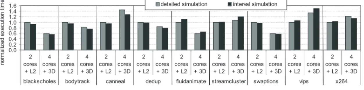
We now consider a case study to illustrate the applica-bility of interval simulation in a practical research study. Our case study considers a performance trade-off as a result of 3D stacking [19], and compares two processor architec-tures. Our first processor architecture is a dual-core pro-cessor with a 4MB L2 cache that is connected to external DRAM through a 16-byte wide memory bus; our second processor architecture is a quad-core processor that is con-nected to 3D stacked DRAM through a 128-byte memory bus and which does not have an L2 cache. External DRAM is assumed to have a 150-cycle access latency; 3D-stacked DRAM is assumed to have a 125-cycle access latency. The important observation from Figure 8 is that interval simula-tion leads to the same conclusions as detailed cycle-accurate simulation. The quad-core processor leads to better perfor-mance for a number of benchmarks, such asbodytrack, flu-idanimateandswaptions; these benchmarks benefit from increased compute power and/or memory bandwidth. For
other benchmarks on the other hand, cache space is more important than processing power and memory bandwidth, and hence, the dual-core processor outperforms the quad-core processor, see canneal, vipsand x264. This case study illustrates that interval simulation leads to the same conclusions in practical high-level microarchitecture design trade-offs.
5.5
Simulation speed
Interval simulation is substantially faster than detailed cycle-level simulation, see Figures 9 and 10, which show the simulation speedup through interval simulation com-pared to detailed simulation for the multi-program work-loads and multi-threaded workwork-loads, respectively. The sim-ulation speedup is a factor 8 to 9×for the multi-threaded workloads, and up to 15×for the multi-program workloads.
6
Related Work
Detailed cycle-level simulation. Architects in industry and academia rely heavily on cycle-level (and in some cases
0.0 0.2 0.4 0.6 0.8 1.0 1.2 1.4 1.6 2 cores + L2 4 cores + 3D 2 cores + L2 4 cores + 3D 2 cores + L2 4 cores + 3D 2 cores + L2 4 cores + 3D 2 cores + L2 4 cores + 3D 2 cores + L2 4 cores + 3D 2 cores + L2 4 cores + 3D 2 cores + L2 4 cores + 3D 2 cores + L2 4 cores + 3D
blackscholes bodytrack canneal dedup fluidanimate streamcluster swaptions vips x264
n o rm a liz e d e x e c u ti o n ti m e
detailed simulation interval simulation
Figure 8. Evaluating interval simulation in a practical design trade-off: a dual-core processor with 4MB L2 and external DRAM versus a quad-core processor with 3D-stacked DRAM and no L2 cache. Performance numbers are normalized to detailed simulation of the dual-core processor configura-tion. 0 5 10 15 20 25 30 35 b z ip 2 c ra ft y e o n g a p g c c g z ip m c f p a rs e r p e rl b m k tw o lf v o rt e x v p r a m m p a p p lu a p s i a rt e q u a k e fa c e re c fm a 3 d g a lg e l lu c a s m e s a m g ri d s ix tr a c k s w im w u p w is a v e ra g e s im u la ti o n s p e e d u p
single-core dual-core quad-core eight-core
Figure 9. Simulation speedup compared to detailed cycle-accurate simulation for SPEC CPU2000. 0 2 4 6 8 10 12 14 16 b la c k s h o le s b o d y tr a c k c a n n e a l d e d u p fl u id a n im a te s tr e a m c lu s te r s w a p ti o n s v ip s x 2 6 4 a v g s im u la ti o n s p e e d u
p single-core dual-core quad-core eight-core
Figure 10. Simulation speedup compared to detailed cycle-accurate simulation for PAR-SEC.
true accurate) simulators. The limitation of cycle-level simulation is that it is very time-consuming. Industry single-core simulators typically run at a speed of 1KHz to 10KHz; academic simulators typically run at tens to hun-dreds of KIPS [4]. Multi-core processor simulators
exacer-bate the problem even further because they have to simulate multiple cores, and have to model inter-core communication (e.g., cache coherence traffic) as well as resource contention in shared resources. In addition, the development effort and time of detailed simulators is a concern. For these rea-sons, it is not uncommon that architects make simplifying assumptions when simulating large core and multi-processor systems. A common assumption is to assume that all cores execute one instruction per cycle (i.e., a non-memory IPC equal to one), see for example [13, 17, 22]. Interval simulation is an easy-to-implement, fast and more accurate alternative for the one-IPC performance model.
Sampled simulation. The idea of sampled simulation is to simulate a number of sampling units rather than the en-tire dynamic instruction stream. The sampling units are selected either randomly (Conte et al. [6]), or periodically (SMARTS, Wunderlich et al. [33]), or based on phase anal-ysis (SimPoint, Sherwood et al. [28]). A number of papers have been working on sampled simulation of multi-threaded and multi-core processors. Van Biesbrouck et al. [30] pro-pose the co-phase matrix for speeding up sampled simulta-neous multithreading (SMT) processor simulation running multi-program workloads. Ekman and Stenstr¨om [8] make the observation that fewer sampling units need to be taken to estimate overall performance for larger multi-processor systems than for smaller multi-processor systems in case one is interested in aggregate performance only. Wenisch et al. [32] obtained similar conclusions for throughput server workloads. Barr et al. [1] propose the Memory Timestamp Record (MTR) to store microarchitecture state (cache and directory state) at the beginning of a sampling unit as a checkpoint. Interval simulation is orthogonal to sampled simulation: sampled simulation reduces the number of in-structions that need to be simulated; interval simulation on the other hand models core-level performance through ana-lytical modeling.
FPGA-accelerated simulation. FPGA-accelerated simu-lation [4, 26, 27, 31] speeds up simusimu-lation by mapping timing models onto field-programmable gate-arrays (FP-GAs). The timing models in FPGA-accelerated simulators are cycle-accurate, and the simulation speedup comes from exploiting fine-grain parallelism in the FPGA. Interval sim-ulation takes a different approach to speeding up simula-tion by analytically modeling core-level performance. In fact, interval simulation could be used in conjunction with FPGA-accelerated simulation, i.e., the cycle-accurate tim-ing models could be replaced by analytical timtim-ing mod-els. This would not only speedup FPGA-based simulation, it would also shorten FPGA-model development time and in addition it would also enable simulating larger computer systems on a single FPGA.
Statistical simulation. Statistical performance modeling has a gained a lot of interest over the past few years. Sta-tistical simulation [7, 23, 25] speeds up architectural simu-lation by providing short-running synthetic traces or bench-marks that are representative for long-running benchbench-marks. This is done by profiling the execution of the original bench-mark and capturing the key execution characteristics in the form of a statistical profile. A synthetic trace or bench-mark is then generated from this statistical profile. By construction, the synthetic clone exhibits similar execution characteristics as the original benchmark. Nussbaum and Smith [24] and Hughes and Li [15] apply the statistical simulation paradigm to multithreaded programs running on shared-memory multiprocessor (SMP) systems. To do so, they extended statistical simulation to model synchroniza-tion and accesses to shared memory. Genbrugge and Eeck-hout [12] show what execution characteristics to measure in the statistical profile in order to be able to accurately sim-ulate shared resources in multi-core processors. The key benefit of statistical simulation is that the synthetic clone’s dynamic instruction count is several orders of magnitude smaller than is the case for the original benchmark, which leads to dramatic reductions in simulation time. Interval simulation is orthogonal to statistical simulation: statistical simulation reduces simulation time by reducing the number of instructions that need to be simulated, whereas interval simulation reduces simulation time by raising the level of abstraction in the simulation model.
Analytical modeling. There are basically three ap-proaches to analytical performance modeling: tic modeling, empirical modeling and hybrid mechanis-tic/empirical modeling. Mechanistic modeling [9, 11, 18, 29] constructs a model based on the mechanics of the target processor, i.e., white-box modeling. The first-order core-level performance model by Eyerman et al. [11] serves as the basis for interval simulation. Empirical modeling learns a performance model through training and does not assume specific knowledge about the target processor, i.e.,
black-box modeling. Ipek et al. [16] learn a model through neural networks, and Lee and Brooks [20] build a model through regression modeling. Lee et al. [21] leverage regression modeling to predict multiprocessor performance running multi-program workloads. Hybrid mechanistic/empirical modeling proposes a mechanistic performance formula in which the parameters are derived through empirical model-ing, see the pipeline model by Hartstein and Puzak [14] as an example.
7
Conclusion
This paper proposed interval simulation which raises the level of abstraction in multi-core architectural simulation. Interval simulation replaces the core-level cycle-accurate simulation model in a multi-core simulator by a mechanistic analytical model. The analytical model estimates core-level performance by dividing the execution in so called inter-vals. The intervals are separated by miss events, i.e., branch mispredictions, TLB misses and cache misses (e.g., conflict misses, coherence misses, etc.). The miss events are de-termined through branch predictor and memory hierarchy simulation; the impact of these miss events on core-level performance is determined through analytical modeling.
Using multi-program SPEC CPU2000 workloads as well as multi-threaded PARSEC benchmarks, and the M5 full-system simulator, we demonstrate the accuracy of multi-core interval simulation: we report average errors around 4% for multi-program SPEC CPU2000 workloads; for the multi-threaded full-system PARSEC benchmarks, the aver-age error is 4.6% (max error of 11%) for up to eight cores. Interval simulation achieves a simulation speedup of one order of magnitude compared to cycle-accurate simulation. Moreover, interval simulation is easy to implement: our implementation of the analytical model is about one thou-sand lines of code, which is a dramatic reduction compared to a detailed cycle-level out-of-order processor simulation model (e.g., 28 thousand lines of code for the out-of-order core model in M5).
We believe that interval simulation is widely applica-ble. We view interval simulation as a useful complement to cycle-accurate simulation for design studies that do not need cycle-accurate timing at the core level, e.g., when making design decisions in early stages of the design or when making system-level and high-level microarchitec-ture design trade-offs or when simulating very large servers. Moreover, interval simulation is orthogonal to existing sim-ulation speedup approaches such as sampled simsim-ulation and FPGA-accelerated simulation.
Acknowledgements
The authors would like to thank the anonymous review-ers for their valuable comments and suggestions. Stijn Ey-erman is a Postdoctoral Fellow with the Fund for Scientific
Research in Flanders (Belgium) (FWO Vlaanderen). Addi-tional support is provided by the FWO projects G.0232.06 and G.0255.08, and the UGent-BOF projects 01J14407 and 01Z04109.
References
[1] K. C. Barr, H. Pan, M. Zhang, and K. Asanovic. Acceler-ating multiprocessor simulation with a memory timestamp record. In ISPASS, pages 66–77, Mar. 2005.
[2] C. Bienia, S. Kumar, J. P. Singh, and K. Li. The PARSEC benchmark suite: Characterization and architectural impli-cations. In PACT, pages 72–81, Oct. 2008.
[3] N. L. Binkert, R. G. Dreslinski, L. R. Hsu, K. T. Lim, A. G. Saidi, and S. K. Reinhardt. The M5 simulator: Modeling networked systems. IEEE Micro, 26(4):52–60, 2006. [4] D. Chiou, D. Sunwoo, J. Kim, N. A. Patil, W. Reinhart,
D. E. Johnson, J. Keefe, and H. Angepat. FPGA-accelerated simulation technologies (FAST): Fast, full-system, cycle-accurate simulators. In MICRO, pages 249–261, Dec. 2007. [5] Y. Chou, B. Fahs, and S. Abraham. Microarchitecture opti-mizations for exploiting memory-level parallelism. In ISCA, pages 76–87, June 2004.
[6] T. M. Conte, M. A. Hirsch, and K. N. Menezes. Reducing state loss for effective trace sampling of superscalar proces-sors. In ICCD, pages 468–477, Oct. 1996.
[7] L. Eeckhout, R. H. Bell Jr., B. Stougie, K. De Bosschere, and L. K. John. Control flow modeling in statistical simulation for accurate and efficient processor design studies. In ISCA, pages 350–361, June 2004.
[8] M. Ekman and P. Stenstr¨om. Enhancing multiprocessor ar-chitecture simulation speed using matched-pair comparison. In ISPASS, pages 89–99, Mar. 2005.
[9] P. G. Emma. Understanding some simple
processor-performance limits. IBM Journal of Research and
Devel-opment, 41(3):215–232, May 1997.
[10] S. Eyerman and L. Eeckhout. System-level
perfor-mance metrics for multi-program workloads. IEEE Micro, 28(3):42–53, May/June 2008.
[11] S. Eyerman, L. Eeckhout, T. Karkhanis, and J. E. Smith. A mechanistic performance model for superscalar out-of-order processors. ACM Transactions on Computer Systems
(TOCS), 27(2), May 2009.
[12] D. Genbrugge and L. Eeckhout. Chip multiprocessor de-sign space exploration through statistical simulation. IEEE
Transactions on Computers, 58(12):1668–1681, Dec. 2009.
[13] L. Hammond, V. Wong, M. Chen, B. D. Carlstrom, J. D. D. an B. Hertzberg, M. K. Prabhu, H. Wijaya, C. Kozyrakis, and K. Olukotun. Transactional memory coherence and con-sistency. In ISCA, pages 102–113, June 2004.
[14] A. Hartstein and T. R. Puzak. The optimal pipeline depth for a microprocessor. In ISCA, pages 7–13, May 2002. [15] C. Hughes and T. Li. Accelerating multi-core processor
de-sign space evaluation using automatic multi-threaded work-load synthesis. In IISWC, pages 163–172, Sept. 2008. [16] E. Ipek, S. A. McKee, B. R. de Supinski, M. Schulz, and
R. Caruana. Efficiently exploring architectural design spaces via predictive modeling. In ASPLOS, pages 195–206, Oct. 2006.
[17] A. Jaleel, W. Hasenplaugh, M. Qureshi, J. Sebot, S. Steely, Jr., and J. S. Emer. Adaptive insertion policies for managing shared caches. In PACT, pages 208–219, Oct. 2008. [18] T. Karkhanis and J. E. Smith. A first-order superscalar
pro-cessor model. In ISCA, pages 338–349, June 2004. [19] T. Kgil, S. D’Souza, A. Saidi, B. N, R. Dreslinski, S.
Rein-hardt, K. Flautner, and T. Mudge. PicoServer: Using 3D stacking technology to enable a compact energy efficient chip multiprocessor. In ASPLOS, pages 117–128, Oct. 2006. [20] B. Lee and D. Brooks. Accurate and efficient regression modeling for microarchitectural performance and power prediction. In ASPLOS, pages 185–194, Oct. 2006. [21] B. Lee, J. Collins, H. Wang, and D. Brooks. CPR:
Com-posable performance regression for scalable multiprocessor models. In MICRO, pages 270–281, Nov. 2008.
[22] K. E. Moore, J. Bobba, M. J. Moravan, M. D. Hill, and D. A. Wood. LogTM: Log-based transactional memory. In HPCA, pages 254–265, Feb. 2006.
[23] S. Nussbaum and J. E. Smith. Modeling superscalar proces-sors via statistical simulation. In PACT, pages 15–24, Sept. 2001.
[24] S. Nussbaum and J. E. Smith. Statistical simulation of sym-metric multiprocessor systems. In ANSS, pages 89–97, Apr. 2002.
[25] M. Oskin, F. T. Chong, and M. Farrens. HLS: Combining statistical and symbolic simulation to guide microprocessor design. In ISCA, pages 71–82, June 2000.
[26] M. Pellauer, M. Vijayaraghavan, M. Adler, Arvind, and J. S. Emer. Quick performance models quickly: Closely-coupled partitioned simulation on FPGAs. In ISPASS, pages 1–10, Apr. 2008.
[27] D. A. Penry, D. Fay, D. Hodgdon, R. Wells, G. Schelle, D. I. August, and D. Connors. Exploiting parallelism and struc-ture to accelerate the simulation of chip multi-processors. In
HPCA, pages 27–38, Feb. 2006.
[28] T. Sherwood, E. Perelman, G. Hamerly, and B. Calder. Au-tomatically characterizing large scale program behavior. In
ASPLOS, pages 45–57, Oct. 2002.
[29] D. J. Sorin, V. S. Pai, S. V. Adve, M. K. Vernon, and D. A. Wood. Analytic evaluation of shared-memory systems with ILP processors. In ISCA, pages 380–391, June 1998. [30] M. Van Biesbrouck, T. Sherwood, and B. Calder. A co-phase
matrix to guide simultaneous multithreading simulation. In
ISPASS, pages 45–56, Mar. 2004.
[31] J. Wawrzynek, D. Patterson, M. Oskin, S.-L. Lu,
C. Kozyrakis, J. C. Hoe, D. Chiou, and K. Asanovic. RAMP: Research accelerator for multiple processors. IEEE Micro, 27(2):46–57, Mar. 2007.
[32] T. F. Wenisch, R. E. Wunderlich, M. Ferdman, A. Ailamaki, B. Falsafi, and J. C. Hoe. SimFlex: Statistical sampling of computer system simulation. IEEE Micro, 26(4):18–31, July 2006.
[33] R. E. Wunderlich, T. F. Wenisch, B. Falsafi, and J. C. Hoe. SMARTS: Accelerating microarchitecture simulation via rigorous statistical sampling. In ISCA, pages 84–95, June 2003.