Subgroup Discovery with Proper Scoring Rules

with Proper Scoring Rules. In Machine Learning and Knowledge Discovery

in Databases : European Conference, ECML PKDD 2016. (pp. 492-510).

(Lecture Notes in Computer Science; Vol. 9852). Springer. DOI:

10.1007/978-3-319-46227-1_31

Peer reviewed version

Link to published version (if available):

10.1007/978-3-319-46227-1_31

Link to publication record in Explore Bristol Research

PDF-document

This is the accepted author manuscript (AAM). The final published version (version of record) is available online via Sprimger Verlag at DOI: 10.1007/978-3-319-46227-1_31. Please refer to any applicable terms of use of the publisher.

University of Bristol - Explore Bristol Research

General rights

This document is made available in accordance with publisher policies. Please cite only the published

version using the reference above. Full terms of use are available:

Hao Song1, Meelis Kull1, Peter Flach1, and Georgios Kalogridis2

1 _{Intelligent Systems Laboratory, University of Bristol, Bristol, UK}

{Hao.Song,Meelis.Kull,Peter.Flach}@bristol.ac.uk

2 _{Toshiba Research Europe Ltd, Telecommunications Research Laboratory, Bristol, UK}

[email protected]

Abstract. Subgroup Discovery is the process of finding and describing suffi-ciently large subsets of a given population that have unusual distributional char-acteristics with regard to some target attribute. Such subgroups can be used as a statistical summary which improves on the default summary of stating the over-all distribution in the population. A natural way to evaluate such summaries is to quantify the difference between predicted and empirical distribution of the target. In this paper we propose to use proper scoring rules, a well-known fam-ily of evaluation measures for assessing the goodness of probability estimators, to obtain theoretically well-founded evaluation measures for subgroup discov-ery. From this perspective, one subgroup is better than another if it has lower divergence of target probability estimates from the actual labels on average. We demonstrate empirically on both synthetic and real-world data that this leads to higher quality statistical summaries than the existing methods based on measures such as Weighted Relative Accuracy.

1

Introduction

Statistical models intend to capture the distributional information in a domain of in-terest. While a global statistical model is useful, it is often also of interest to capture local variations exhibited in a subset of the data. Recognising such subsets can provide valuable knowledge and opportunities to improve performance at tasks relying on the statistical model. In the area of machine learning and data mining, the problem of ob-taining such statistically different subsets is known as Subgroup Discovery (SD) [7, 17, 10, 6], loosely defined as the process of finding and describing sufficiently large sub-sets of a given population that have unusual distributional characteristics with regard to some target attribute.

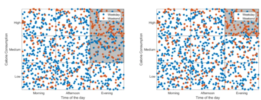
Consider a synthetic toy data set relating to someone’s dietary habits. It contains two (discretised) features: the time of the day, denoted asX1∈ {Morning,Afternoon, Evening} and the calorie consumption in the diet, denoted as X2∈ {Low,Medium, High}. The target variable isY ∈ {Weekday,Weekend}. Figure 1 visualises the data, with two potentially interesting subgroups (shaded areas). The subgroup on the right concentrates on the area of maximum statistical deviation (high calorie intake in the evening is more common during weekend), while the one on the left covers both medium and high calorie intake in the evening. In this paper we study reasons why one of these subgroups might be preferred over the other.

Fig. 1: An example bivariate data set with two subgroups (shaded areas) defined on the discretised features, both capturing an area of statistical deviation in comparison to the overall population. The subgroup on the left is preferred by a commonly used evaluation measure (WRAcc) while the right subgroup is preferred by the one of the measures we propose in this paper.

Clearly, if a subgroup is small, distributional differences may arise purely because of random chance in sampling, so a trade-off between subgroup size and distributional deviation needs to be made. Statistical tests such asχ2can be used, but are usually

over-emphasising size: a very large subgroup with small deviation is more likely to be picked up than a medium-sized subgroup with considerable deviation. p-values as reported in rule-based approaches [10] tend to suffer from the same issue.

Historically, SD developed as a variation on rule-learning and other logic-based approaches, and hence it is not surprising that many existing quality measures have been adapted from decision trees and rule-based classifiers. For instance, [1] explored the use of Gini-split (among several others) as quality measure for subgroups, which hypothesises that a good binary split in a decision tree also establishes a good subgroup. One of the most commonly used measures is Weighted Relative Accuracy (WRAcc), which can be seen as an adaptation of precision, a measure that is used as a search heuristic in rule learners such as CN2 [3]. Many other subgroup quality measures have been introduced in the literature, see [6] for an overview.

Evaluation methods for SD depend on the task for which subgroups need to be found. In [10], the subgroups are used to construct a ranking model, and the area un-der the corresponding ROC curve is used as an evaluation measure. In [1] the obtained subgroups are used as features for a decision tree and hence they can be evaluated ac-cording to the classification performance of the trees. However, the predictive task used in evaluation (ranking or classification) is then different from the descriptive Subgroup Discovery (SD) task, and it is unclear how the predictive task affects the choice of subgroup quality measure.

In this paper we propose a novel approach to evaluate subgroups as summaries which improve on the default summary of stating the overall distribution in the popu-lation. A natural way to evaluate such summaries is to quantify the difference between predicted and empirical distribution of the target. This obviates the use of proper scoring rules, a well-known family of evaluation measures for assessing the goodness of

proba-bility estimators, to obtain theoretically well-founded evaluation measures for subgroup discovery. From this perspective, one subgroup is better than another if it on average has lower divergence of target probability estimates from the actual labels.

We derive a novel SD method to directly optimise for the proposed evaluation mea-sure, from first principles. The method is based on a generative probabilistic model, which allows us to formally prove the validity of the method. We perform experiments on a synthetic data set where the theoretically optimal subgroup is known, and demon-strate that our method outperforms alternative methods in the sense that it finds sub-groups that are closer to the theoretically optimal one. Additionally, we perform exper-iments on 20 UCI data sets which demonstrate that the proposed method is superior in summarising the statistical properties of the data.

The structure of this paper is as follows. Section 2 introduces the notations and concepts for SD. Section 3 provides an overview of Proper Scoring Rules (PSRs) and describes related quality measures. In Section 4 we propose a novel generative mod-elling approach to address the summarisation problem, and derive the corresponding measures. Section 5 evaluates the proposed quality measures against existing measures and Section 6 presents related work. Section 7 concludes this paper and discusses pos-sible future research directions.

2

Subgroup Discovery

We start by introducing some notation. Consider a dataset(Xi,Yi),i=1, . . . ,nin the

in-stance space(X,Y). We assume a multi-class target variable, representing thekclasses

inYby unit vectors, i.e. class jis represented by the vector with 1 at position jand

0 everywhere else. The set of all considered subgroups is indicated byG⊂2X. This

set is typically generated by asubgroup language(e.g., the set of all conjunctions over some fixed set of literals) but here it suffices to deal with subgroups extensionally. A subgroupg∈Gcan then be identified with its characteristic functiong:X→ {0,1}

determining whether an instanceXiis in the subgroup (g(Xi) =1) or not (g(Xi) =0).

A subgroup quality measure is a functionφ:G→Rsuch that better subgroupsgget a

higherφ(g). The task of SD is then to find the subgroupg∗with the highest value ofφ, i.e.g∗=arg max_g∈Gφ(g).

A wide range of proposed quality measures can be found in the literature. The com-mon way of defining a quality measure is to separate them into two factors: the deviation factor and the size factor. The deviation factor is in charge of comparing the local statis-tic to the global statisstatis-tic. In the case of a discrete target variable, the deviation factor can be seen as a function that takes two estimates of class probabilities as input and outputs a single number to indicate how different these two estimates are. The size factor is normally treated as a correction term to encourage the method to find larger subgroups, as small subgroups tend to be less valuable.

One of the most widely adopted quality measures is the Weighted Relative Accu-racy (WRAcc) family [1, 2, 9, 10]. For a binary target this essentially is the covariance between the target variable and subgroup membership: since these are both Bernoulli variables this takes values in the interval[−0.25,0.25]. For a multi-class target we take the average of all one-against-rest binary WRAcc values, taking the absolute value of

the latter to avoid positive and negative covariances cancelling out [1]. For our purposes we derive a related but unnormalised quantity, as follows.

Denote the overall class distribution in the data set byπ= (∑ni=1Yi)/n(note thatYi

andπare vectors of lengthk). Letmdenote the number of training set instances

belong-ing to the subgroupg, i.e.m=∑ni=1g(Xi). Denote the class distribution in the subgroup

byρ(g), i.e.,ρ(g)= (∑ni=1g(Xi)·Yi)/m. Then an unnormalised version of Multi-class

Weighted Relative Accuracy (MWRAcc) can be calculated as:

φMW RAcc(g) =m· k

∑

|ρ(_jg)−πj| (1)

The definition of [1] is obtained from this by normalising with n·k, wheren is the number of training instances andkis the number of classes (both constant). Our version can be interpreted as absolute differences between observed and expected counts.

3

Proper Scoring Rules

The class distributionπ is a very simple way to summarise the target variable across

the whole training dataset. That is, we summarise the labels vectorsY1, . . . ,Ynwith the

summarySπ_{where we defineS}π

i =πfori=1, . . . ,n. Another possibility is to separately

summarise a particular subgroupgwith its class distributionρ(g)while its complement is summarised withπ. We denote this summary bySg,ρ(g),π, and for an instanceithis summary predictsSg_i,ρ(g),π=ρ(g)ifg(Xi) =1 andSg,ρ

(g)_,π

i =πifg(Xi) =0, which can

be jointly written asSg_i,ρ(g),π =ρ(g)g(Xi) +π(1−g(Xi)). One could then ask which

of the subgroups gives the best summary, and whether the summary is better than the default summarySπ_{. In order to assess this, we need a way to calculate the extent to}

which the probability estimates within the summary deviate from the actual labels. Proper Scoring Rules (PSRs) have been widely adopted in the area of machine learn-ing and statistics to assess the goodness of probability estimates [16]. A scorlearn-ing rule is a functionψ:S×Y→Rthat assigns a real-valued loss to the estimateSi within the

summarySwith respect to the actual labelYiof instancei. Two of the most commonly

adopted scoring rules are the Brier Score (BS) and Log-loss (LL), which are defined as:

ψBS(Si,Yi) = k

∑

whereYi,j=1 if thei-th instance is of the j-th class and 0 otherwise,Si,jis the

proba-bility estimate of class jfor thei-th instance, andSi,∗denotes the probability estimate

of thei-th instance for the true class as determined byYi.

The distance from a whole summarySto the actual labels can then be calculated as follows: ψ0(S,Y) = n

∑

The scoring rule ψ is proper if arg min_pψ0(Sp,Y) =π for anyY, i.e., if the actual class distribution is the minimiser of the scoring rule. In particular, both BS and LL are proper.

For every proper scoring ruleψ there is a corresponding divergence measure d

which quantifies how much a class probability distribution diverges from another class distribution. Formally, the divergence d(p,q)is the expected value of the difference

ψ(p,Y)−ψ(q,Y)whereY is drawn from the distributionq. The divergences

corre-sponding to BS and LL are the squared error and Kullback-Leibler (KL) divergence, respectively. dBS(p,q) = k

∑

∑

For more details see [8].

3.1 Information Gain

Suppose we now want to decide whether to summarise the whole dataset bySπ _{or by}

Sg,ρ(g),π for someg. For this let us take a proper scoring ruleψ0to quantify the loss of a summary with respect to actual labels. We can now define the quality of a subgroupg

as the gain inψ0of the summarySg,ρ(g),πover the default summarySπ_{, that is:}

φIG(g) =ψ0(Sπ,Y)−ψ0(Sg,ρ

(g)_,π

,Y) (7)

In principle, we could consider summaries Sg,ρ,π for any other class distribution ρ. However, the summary withρ(g) is special among these, as it is maximising the gain over the summarySπ_{due to properness of the scoring rule. This is stated in the}

follow-ing theorem:

Theorem 1. Letψ,ψ0,d be a proper scoring rule, its sum across the dataset, and its

corresponding divergence measure, respectively. Then for any given subgroup g the following holds:

arg max

ρ

ψ0(Sπ,Y)−ψ0(Sg,ρ,π,Y) =ρ(g) (8)

whereρ(g) denotes the class distribution within the subgroup g. The maximum value

achieved is m·d(π,ρ(g))where m is the size of the subgroup g.

Proofs of all theorems are provided in Appendix A.

The theorem implies that Eq.(7) can be rewritten as follows:

φIG(g) =m·d(π,ρ(g)) (9)

In words, this quality measure multiplies the size of the subgroup by the divergence of the overall class distribution from the distribution within the subgroup3.

3_{In general, divergence measures are not symmetric, sod(}

If we consider Log-loss as the proper scoring rule, then the corresponding informa-tion gain measure is:

φIG-LL(g) =m·KL(π,ρ(g)) (10)

whereKLis the KL-divergence. For Brier Score the corresponding measure is quadratic error: φIG-BS(g) =m· k

∑

whereρ(_jg)is the proportion of the j-th class in the subgroupg.

These information gain measures have a long history in machine learning, for exam-ple in decision tree learning where they measure the decrease in impurity when splitting a parent node into two children nodes. If we measure impurity by Shannon entropy this leads to Quinlan’s information gain splitting criterion; and if we measure impurity by the Gini index we obtain Gini-split. We have shown how they can be unified from the perspective of Proper Scoring Rules; we now proceed to improve them.

4

Generative Modelling

The general context in which SD is applied is where one observes a set of data points that belongs to a particular domain and the task is to extract information from the data. As mentioned in the introduction, such information can then be adopted to improve the performance of corresponding applications. Therefore, it is desirable that the subgroups as the representation of obtained knowledge would generalise to future data observed in the same domain.

Two problems need addressing when generalising to future data. First, the class dis-tributionρ(g)is calculated on a (small) sample and can therefore be a poor estimate of

the actual distribution in the future. Second, it is not certain whether the actual distri-bution of the subgroup is different from the overall distridistri-butionπ. In order to capture

these aspects we employ a generative model to generate a newtestinstanceY of the subgroupg. We assume that the observed (training) instances of subgroupgwere gen-erated according to the same model, which is defined as follows.

4.1 The Generative Model

First, we fix the defaultk-class distributionπ. We then decide whether the distribution

of the subgroupgis different from the default (Z=1) or the same as default (Z=0):

Z∼Bernoulli[γ] (12)

whereγis our prior belief thatZ=1. IfZ=1 then we generate the class distributionQ

for the subgroupg:

Q∼Dir[β] (13)

whereDir[β]is thek-dimensional Dirichlet distribution with parameter vectorβ.

all independent and identically distributed (iid). For simplicity of notation, let us assume that the training instances withingare the firstminstancesY1, . . . ,Ym. The distribution

ofY1, . . . ,Ymand the test labelYis as follows:

Y,Y1, . . . ,Ym∼Cat[ZQ+ (1−Z)π] (14)

whereCatis the categorical distribution with the given class probabilities. In the ex-periments reported later we used non-informative priors for Z and Q (γ =0.5 and β = (1, . . . ,1), respectively).

4.2 Proposed Quality Measures

The above model can be used to generate instances for a subgroupg. We will now ex-ploit this model to derive two subgroup quality measures, the first one of which takes into account the uncertainty about the true class distribution in the subgroup, while the second one also models our uncertainty whether it is different from the background distribution. Therefore, we consider the task of choosingρwhich would maximise the expected gain inψ0on thetestinstances. The following theorem solves this task, con-ditioning on the observed class distribution within the subgroup and on the assumption that this subgroup is different from background (Z=1).

Theorem 2. Consider a subgroup as generated with the model above. Denote the counts

of each class in the training set of this subgroup by C=∑mi=1Yi. Then

arg max

ρ

E[ψ0(π,Y)−ψ0(ρ,Y)|C=c,Z=1] = c+β

∑kj=1cj+βj

(15)

Denoting this quantity byρˆ, the achieved maximum is d(π,ρˆ), where d is the divergence measure corresponding toψ.

In the experiments we useβ= (1, . . . ,1)and hence the gain is maximised when predict-ing the Laplace-corrected probabilities, i.e., addpredict-ing 1 to all counts and then normalispredict-ing. According to this theorem we propose a novel quality measure which takes into account the uncertainty about the class distribution:

φd(g) =m·d(π,ρˆ) (16)

wheremis the size of the subgroup.

The following theorem differs from the previous theorem by not conditioning on

Z=1. Hence, it additionally takes into account the uncertainty about whether the dis-tribution of the subgroup is different from the background.

Theorem 3. Consider a subgroup as generated with the model above and denote C as

above. Then arg max ρ E[ψ0(π,Y)−ψ0(ρ,Y)|C=c] =a c+β ∑kj=1cj+βj + (1−a)π (17)

where a=_P[Z=1|C=c]. Denote this quantity byρˆˆ. Then the achieved maximum value

Following this theorem we propose another novel quality measure, which takes into account both the uncertainty about the class distribution and about whether it is different from the background distribution:

φPSR(g) =m·d(π,ρˆˆ) (18)

wheremis the size of the subgroup. In order to calculate the value ofa=P[Z=1|C=c]

we have the following theorem:

Theorem 4. Consider a subgroup as generated with the model above and denote C as

above. Then the following equalities hold:

P[Z=1|C=c] = γ·P[C=c|Z=1] γ·P[C=c|Z=1] + (1−γ)·P[C=c|Z=0] P[C=c|Z=1] = m c ·Γ(∑ k j=1βj) ∏kj=1Γ(βj) ·∏ k j=1Γ(cj+βj) Γ(m+β0) P[C=c|Z=0] = m c · k

∏

Referring back to Figure 1 in the introduction, the subgroup on the left was discov-ered withφW RAccas quality measure and the right one byφPSRwith Brier Score. While

WRAcc provides a larger coverage, it can be seen that the PSR measure captures a more distinct statistical deviation of the class distribution in the subgroup.

5

Experiments

In this section we experimentally investigate the performance of our proposed measures. The experiments are separated into two parts. For the first part we generated synthetic data, such that we know the true subgroup. In the second part we applied our methods to UCI data to investigate summarisation performance.

For our proposed measures, we adopt the generalised divergences of BS and LL as given in Section 3, Eqs.(5-6). Plugging these into Eqs.(16) and (18) we obtain four novel measures d-BS, d-LL, PSR-BS and PSR-LL. We compare these proposals against a range of subgroup evaluation measures used in the literature: Weighted Relative Ac-curacy (WRAcc), IG-LL (Eq.(10)), IG-BS (Eq.(11)), as well as theχ2statistic, which

is defined as follows: φChi2=C· K

∑

In the experiments on the synthetic data we evaluate how good the methods are in revealing the true subgroup used in generating the data, as well as in producing good summaries of the data.

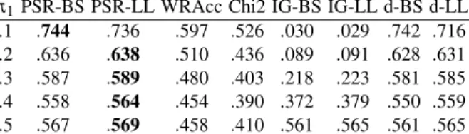
π1PSR-BS PSR-LL WRAcc Chi2 IG-BS IG-LL d-BS d-LL .1 .744 .736 .597 .526 .030 .029 .742 .716 .2 .636 .638 .510 .436 .089 .091 .628 .631 .3 .587 .589 .480 .403 .218 .223 .581 .585 .4 .558 .564 .454 .390 .372 .379 .550 .559 .5 .567 .569 .458 .410 .561 .565 .561 .565

Table 1: Micro-averaged F-scores on the artificial data, for different class distributions (π1). The best results for each row are shown in bold.

To provide a more intuitive illustration, we construct our data set according to a real-life scenario. Suppose one has been using a wearable device to record whether daily exercises were performed or not, for a whole year. As it turned out, there were 146 out of 365 days when the exercises were performed, which gives a probability about 2/5 that the exercises were performed on a random day. According to the website of the wearable device, the same statistics are about 1/3 for the general population. It is possible that the overall exercise frequency was different, but perhaps a more plausible explanation might be that more exercises were performed during a particular period only. SD can hence be applied to recognise the period of more intensive exercise and summarise the corresponding exercise frequency.

Following this scenario, the feature space consists of the 52 weeks of the year, hence_X={1, ...,52}. We define the subgroup language as the set of all intervals of weeks of length from 2 to 8 weeks. The data set is assumed to contain a single year from January to December. This setting allows us to perform exhaustive search on the subgroup language. As here our aim is to compare the performance among different quality measures, applying exhaustive search can avoid the bias introduced by other greedy search algorithms.

The way to generate the data is then as described in the previous section. Given the default class distributionπ, the subgroup class distributionQis sampled from a Dirichlet prior and a true subgroup is selected uniformly within the language. Therefore, all the 7 days within each week can be distributed either according toπor according to

Q.

We evaluate each subgroup quality measure by comparing the obtained subgroup against the true subgroup. This is done by measuring similarity of the respective indica-tor functionsZand ˆZ. For similarity we use the F-score as we are not really interested in the ‘true negatives’ (instances in the complements of both true and discovered sub-groups). The F-score for this case can be computed as (Ziand ˆZiare used to represent

whether an instance belongs to the true subgroup and the obtained subgroup respec-tively):

F1=

2·∑Ni=1I(Zi=1,Zˆi=1)

∑Ni=1(2·I(Zi=1,Zˆi=1) +I(Zi=1,Zˆi=0) +I(Zi=0,Zˆi=1))

(21)

The results are given in Table 1 as the micro-averaged F-scores from 5 000 synthetic sequences, for different values ofπ1(the first component of the class distribution

π1 PSR-BS PSR-LL WRAcc Chi2 IG-BS IG-LL d-BS d-LL .1 .195±.03.195±.03.207±.03.212±.03.231±.04.231±.04.195±.03.195±.03 .2 .326±.03.326±.03.334±.03.337±.03.350±.04.350±.04.326±.03.326±.03 .3 .419±.02.419±.02.424±.02.426±.02.430±.03.430±.03.420±.02.420±.02 .4 .475±.02.475±.02.479±.02.480±.01.478±.02.478±.02.476±.02.476±.02 .5 .494±.02.494±.02.497±.01.498±.01.494±.02.495±.02.494±.02.494±.02

Table 2: Average Brier scores on the artificial data. The best results are shown in bold.

π1 PSR-BS PSR-LL WRAcc Chi2 IG-BS IG-LL d-BS d-LL

.1 .344±.04.344±.04.359±.04.368±.04.406±.06.407±.06.344±.04.347±.04 .2 .507±.03.507±.03.517±.03.520±.03.539±.05.540±.05.508±.03.509±.03 .3 .610±.03.610±.03.616±.02.618±.02.624±.03.624±.03.611±.03.611±.03 .4 .668±.02.668±.02.673±.02.674±.02.671±.02.671±.02.670±.02.669±.02 .5 .687±.02.686±.02.690±.01.691±.01.688±.02.687±.02.688±.02.687±.02

Table 3: Average Log-loss on the artificial data. The best results are shown in bold.

with a slight advantage for Log-loss over Brier score. The information gain-based meth-ods perform particularly poorly, as they have a preference for pure subgroups, whereas for skewedπit would be advantageous to look for subgroups with a more uniform class

distribution. Asπ becomes more uniform, the ‘true’ subgroup becomes more random

and harder to identify, which is why all methods are expected to perform poorly for

π1≈0.5. The variance is quite high across all methods, probably because the data set

is quite small (52·7=364 instances).

Since a better statistical summary is essentially our aim, the results are also evalu-ated according to their overall loss on a test set (also of length 1 year) drawn from the same distribution. For each quality measure, a subgroup is obtained from the training fold together with the local statistical summary ( ˆˆρ forφPSR, ˆρ for other quality

mea-sures). The loss for the obtained summarisation can then be calculated as in Eq.(4). The corresponding results are given in Tables 2-3 for both Brier score and Log-loss. We see a similar pattern as with the F-score results.

5.2 UCI Data

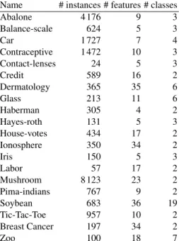
We proceed to compare our method with existing approaches on UCI data sets [13]. We selected the same 20 UCI datasets as described in [1]. The information regarding the number of attributes and instances are provided in the appendix.

The subgroup language we used here is conjunctive normal form, with disjunctions (only) between values of the same feature, and conjunctions among disjunctions in-volving different features. All features are treated as nominal. If the original feature is numeric and contains more than 100 values, it is discretised into 16 bins.

Since for most data sets in this experiment exhaustive search is intractable we per-form beam search instead. The beam width is set to be 32 (i.e., 32 candidate subgroups are kept to be refined in the next round). The number of refinement rounds is set to 8.

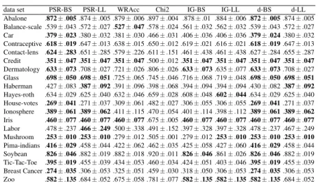
data set PSR-BS PSR-LL WRAcc Chi2 IG-BS IG-LL d-BS d-LL Abalone .872±.005.874±.005.879±.006.897±.004 .878±.01 .884±.006.872±.005.874±.005 Balance-scale.539±.043.572±.027.527±.047.578±.024.561±.032.562±.032.539±.043.572±.027 Car .379±.023.380±.032.381±.030.466±.031.406±.036.406±.036.379±.024.380±.032 Contraceptive.618±.019.647±.013.638±.015.650±.012.619±.021.616±.021.618±.019.647±.013 Contact-lens .624±.283.651±.285.579±.226.611±.151.461±.438.461±.438.627±.284.655±.287 Credit .351±.047.351±.047.351±.047.500±.012.351±.047.351±.047.351±.047.351±.047 Dermatology .633±.073.708±.027.721±.026.806±.026.633±.073.635±.077.633±.073.708±.027 Glass .698±.050.698±.051.725±.065.745±.046.716±.068.719±.048.698±.050.698±.051 Haberman .427±.083.387±.092.391±.096.398±.068.394±.094.394±.094.430±.082.387±.092 Hayes-roth .634±.029.625±.040.632±.046.659±.028.608±.048.602±.044.634±.029.625±.040 House-votes .269±.041.271±.037.309±.061.482±.027.306±.055.306±.055.269±.041.271±.037 Ionosphere .389±.061.389±.062.411±.115.470±.054.401±.114.398±.112.389±.061.389±.062 Iris .460±.077.460±.077.460±.077.675±.005.460±.077.460±.077.460±.077.460±.077 Labor .478±.237.466±.249.500±.338.491±.152.397±.328.397±.328.478±.237.467±.249 Mushroom .253±.010.253±.010.279±.012.505±.001.279±.012.253±.010.253±.010.253±.010 Pima-indians .416±.029.458±.044.422±.062.462±.035.425±.058.427±.060.416±.029.458±.044 Soybean .826±.046.882±.019.882±.018.920±.011.826±.046.861±.026.826±.046.882±.019 Tic-Tac-Toe .395±.019.455±.039.434±.053.460±.034.424±.051.403±.046.395±.019.455±.039 Breast Cancer.274±.035.306±.053.325±.051.459±.030.318±.050.306±.053.274±.035.306±.053 Zoo .582±.135.684±.052.675±.058.781±.077.582±.135.582±.135.582±.135.684±.052

Table 4: Average Brier scores for the UCI data sets. The best results are shown in bold.

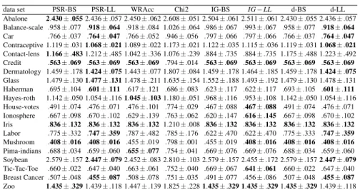
The resulting average Brier scores and Log-loss are given in Tables 4-5. All the results are obtained by 10-fold cross-validation. As in the previous experiment, a sub-group is learned on the training folds and the class distribution estimated on the test fold is then used to compute the corresponding loss.

Given these results, it can be seen that our proposed measures generally outper-form WRAcc,Chi2 and both versions of information gain. The PSR measures (first two columns) are never outperformed by the generalised divergence (last two columns) so we recommend using the former unless simplicity of implementation is an issue (as the latter don’t need estimation ofa). Regarding the choice between (BS,LL), this is still an ongoing debate in the community. Here we used both to demonstrate that our novel measure can apply either as the two most well-known Proper Scoring Rules.

6

Related Work

As is the case for supervised rule learning in general, SD comprises three major compo-nents: description language, quality measure and search algorithm. A detailed compar-ison with rule learning can be found in [15]. While early work in SD has been surveyed in [6], we briefly describe some recent progress in the area.

Regarding the subgroup description language, most existing work defines it through logical operations on attribute values. In [14] the authors present an approach to con-struct more informative descriptions on numeric and nominal attributes in linear time. The proposed algorithm is able to find the optimal interval for numeric attributes and optimal set of values for nominal attributes.The results show improvements on the qual-ity of obtained subgroups comparing to traditional descriptions.

In terms of quality measures, recent work has focused on the extension of tradi-tional measures with improved statistical modelling. In [4, 11] Exceptradi-tional Model Min-ing (EMM) was introduced as a framework to support improved target concepts with

data set PSR-BS PSR-LL WRAcc Chi2 IG-BS IG−LL d-BS d-LL Abalone 2.430±.0552.436±.057 2.450±.062 2.608±.051 2.504±.061 2.511±.061 2.430±.055 2.436±.057 Balance-scale .958±.077 .918±.064 .918±.084 1.026±.064 .986±.067 .993±.067 .958±.077 .918±.064 Car .766±.037 .764±.047 .766±.052 .946±.056 .797±.066 .797±.066 .766±.037 .764±.047 Contraceptive 1.119±.0311.068±.0211.089±.022 1.173±.021 1.122±.035 1.115±.036 1.119±.0311.068±.021 Contact-lens 1.166±.4831.212±.485 1.042±.336 1.076±.239 .884±.735 .884±.735 1.175±.488 1.223±.492 Credit .563±.069 .563±.069 .563±.069 .794±.014 .563±.069 .563±.069 .563±.069 .563±.069 Dermatology 1.459±.1781.424±.0751.443±.077 1.807±.084 1.459±.178 1.464±.185 1.459±.1781.424±.075 Glass 1.479±.1301.477±.1311.478±.211 1.635±.154 1.552±.188 1.493±.192 1.479±.130 1.478±.131 Haberman .695±.104 .601±.111 .617±.121 .686±.083 .623±.117 .622±.117 .693±.105 .601±.111 Hayes-roth 1.142±.050 1.054±.1161.045±.1031.180±.051 .968±.116 .953±.108 1.142±.050 1.054±.116 House-votes .491±.074 .476±.071 .476±.101 .774±.029 .467±.088 .467±.088 .491±.074 .476±.071 Ionosphere .667±.098 .670±.102 .629±.139 .763±.062 .620±.147 .616±.145 .667±.098 .670±.102 Iris .836±.132 .836±.132 .836±.1321.210±.008 .836±.132 .836±.132 .836±.132 .836±.132 Labor .775±.332 .747±.359 .787±.482 .785±.176 .622±.470 .622±.470 .775±.333 .747±.359 Mushroom .408±.016 .408±.016 .455±.019 .798±.001 .455±.019 .408±.016 .408±.016 .408±.016 Pima-indians .688±.034 .659±.060 .655±.077 .754±.041 .669±.076 .669±.076 .688±.034 .659±.060 Soybean 2.579±.1572.447±.0792.452±.083 2.810±.103 2.579±.157 2.455±.172 2.579±.1572.447±.079 Tic-Tac-Toe .660±.022 .647±.040 .663±.061 .752±.040 .669±.067 .641±.061 .660±.022 .647±.040 Breast Cancer .507±.048 .455±.087 .508±.078 .751±.035 .491±.077 .456±.086 .507±.048 .455±.087 Zoo 1.435±.3291.439±.118 1.447±.139 1.825±.2281.435±.329 1.435±.3291.435±.3291.439±.118

Table 5: Average Log-loss for the UCI data sets. The best results are shown in bold.

different model classes. For example, if linear regression models are trained on the whole data set and different candidate subgroups, the quality of subgroups can be eval-uated by comparing the regression coefficient between the global model and the local subgroup model. In [5] the authors extend the framework to support predictive statisti-cal information. This further allows subgroups to be found where a scoring classifier’s performance deviates from its overall performance.

With respect to the search algorithm, while greedy search algorithms have been widely adopted in existing implementations, recent work in [12] presents a fast exhaus-tive search strategy for numerical target concepts. The authors propose and illustrate novel bounds on different types of quality measures. The exhaustive search can then be performed efficiently via additional pruning techniques.

7

Conclusion

In this paper we investigated how to discover subgroups that are optimal in the sense of maximally improving the global statistical summary of a given data set. By assuming that the (discrete) statistical summary is to be evaluated by the Proper Scoring Rule, we derived the corresponding quality measures from first principles. We also proposed a generative model to consider the optimal statistical summary for any candidate sub-group. By performing experiments on both synthetic data and UCI data, we showed that our measures provide better summaries in comparison with existing methods.

The major advantage of adopting our generative model is that it prevents finding small subgroups with extreme distributions. This can be seen as applying a regulari-sation on the class distribution, similar to performing Laplace smoothing in decision tree learning. Given the experiments, we can observe that the novel measures tend to perform better on small data sets (e.g. Contact-lenses, Labor).

Since in this paper we assume that only the subgroup with the highest gain will be discovered, one major direction for further work is to investigate multiple subgroups that can together improve the overall statistical summary. Previous Subgroup Discov-ery algorithms have extended the covering algorithm to weighted covering in order to promote the discovery of overlapping subgroups [10]. We expect that the PSR approach will be able to derive appropriate weight updates in a principled fashion.

Another direction would be to generalise our approach to numeric target variables. Although in general PSRs are designed to work with discrete random variables, Log-loss has been widely adopted in Bayesian analysis, which provides an interface to ex-tend our approach to a general form of statistical modelling.

Acknowledgements This work was supported by the SPHERE Interdisciplinary

Re-search Collaboration, funded by the UK Engineering and Physical Sciences ReRe-search Council under grant EP/K031910/1; and the REFRAME project granted by the Euro-pean Coordinated Research on Long-Term Challenges in Information and Communica-tion Sciences & Technologies ERA-Net (CHIST-ERA), and funded by the Engineering and Physical Sciences Research Council in the UK under grant EP/K018728/1. Hao Song would like to thank Toshiba Research Europe Ltd, Telecommunications Research Laboratory, for funding his doctoral research within SPHERE.

References

1. Abudawood, T., Flach, P.: Evaluation measures for multi-class subgroup discovery. In: Ma-chine Learning and Knowledge Discovery in Databases, pp. 35–50. Springer (2009) 2. Atzmueller, M., Lemmerich, F.: Fast subgroup discovery for continuous target concepts. In:

Foundations of Intelligent Systems, pp. 35–44. Springer (2009)

3. Clark, P., Boswell, R.: Rule induction with CN2: Some recent improvements. In: Machine learning EWSL 91. pp. 151–163. Springer (1991)

4. Duivesteijn, W., Feelders, A.J., Knobbe, A.: Exceptional model mining. Data Mining and Knowledge Discovery pp. 1–52 (2013)

5. Duivesteijn, W., Thaele, J.: Understanding where your classifier does (not) work–the SCaPE model class for EMM. In: Data Mining (ICDM), 2014 IEEE International Conference on. pp. 809–814. IEEE (2014)

6. Herrera, F., Carmona, C.J., Gonz´alez, P., del Jesus, M.J.: An overview on subgroup dis-covery: foundations and applications. Knowledge and information systems 29(3), 495–525 (2011)

7. Kl¨osgen, W.: Explora: A multipattern and multistrategy discovery assistant. In: Fayyad, U.M., Piatetsky-Shapiro, G., Smyth, P., Uthurusamy, R. (eds.) Advances in Knowledge Dis-covery and Data Mining, pp. 249–271. American Association for Artificial Intelligence, Menlo Park, CA, USA (1996)

8. Kull, M., Flach, P.: Novel decompositions of proper scoring rules for classification: Score adjustment as precursor to calibration. In: Machine Learning and Knowledge Discovery in Databases, pp. 68–85. Springer International Publishing (2015)

9. Lavraˇc, N., Flach, P., Zupan, B.: Rule evaluation measures: A unifying view. In: Interna-tional Conference on Inductive Logic Programming. pp. 174–185. Springer Berlin Heidel-berg (1999)

10. Lavraˇc, N., Kavˇsek, B., Flach, P., Todorovski, L.: Subgroup discovery with CN2-SD. The Journal of Machine Learning Research 5, 153–188 (2004)

11. Leman, D., Feelders, A.J., Knobbe, A.: Exceptional model mining. In: Machine Learning and Knowledge Discovery in Databases, pp. 1–16. Springer (2008)

12. Lemmerich, F., Atzmueller, M., Puppe, F.: Fast exhaustive subgroup discovery with numeri-cal target concepts. Data Mining and Knowledge Discovery 30(3), 711–762 (2016) 13. Lichman, M.: UCI machine learning repository (2013), http://archive.ics.uci.edu/ml 14. Mampaey, M., Nijssen, S., Feelders, A., Knobbe, A.: Efficient algorithms for finding richer

subgroup descriptions in numeric and nominal data. In: IEEE International Conference on Data Mining. pp. 499–508 (2012)

15. Novak, P.K., Lavraˇc, N., Webb, G.I.: Supervised descriptive rule discovery: A unifying sur-vey of contrast set, emerging pattern and subgroup mining. The Journal of Machine Learning Research 10, 377–403 (2009)

16. Winkler, R.L.: Scoring rules and the evaluation of probability assessors. Journal of the Amer-ican Statistical Association 64(327), 1073–1078 (1969)

17. Wrobel, S.: An algorithm for multi-relational discovery of subgroups. In: Principles of Data Mining and Knowledge Discovery, pp. 78–87. Springer (1997)

Appendix A: Proofs

Lemma 1. Letψ be a proper scoring rule and d its respective divergence measure.

If S,S0 are random vectors representing two sets of class probability estimates for a random variable T representing the actual class, then

E[ψ(S,T)−ψ(S0,T)] =_E[d(S,T)−d(S0,T)] =_E[d(S,_E[T])−d(S0,_E[T])] (22)

Proof. By using Lemma 1 from the supplementary of [8] we get the decomposition

E[ψ(S,T)] =E[d(S,T)] =E[d(S,E[T])] +E[d(E[T],T)]and the analogous

decompo-sition forS0. The second term is shared and hence when subtracting it cancels, yielding the required result.

Theorem 1. Letψ,ψ0,d be a proper scoring rule, its sum across the dataset, and its

corresponding divergence measure, respectively. Then for any given subgroup g the following holds:

arg max

ρ

ψ0(Sπ_,Y)−

ψ0(Sg,ρ,π,Y) =ρ(g) (23)

whereρ(g) denotes the class distribution within the subgroup g. The value of achieved maximum is m·d(π,ρ(g))where m is the size of the subgroup g.

Proof. For simplicity of notation, let us assume that the training instances withing

areY1, . . . ,Ym(the firstminstances). Consider a random variableT obtaining its value

by uniformly choosing oneYi that belongs tog amongY1, . . . ,Ym. The summariesSπ

andSg,ρ(g),π are equal for instancesm+1, . . . ,n, henceψ0(Sπ_,Y)−ψ0_(Sg,ρ(g)_,π ,Y) = m·_E[ψ(π,T)−ψ(ρ(g),T)]. Using Lemma 1 this is in turn equal tom·_E[d(π,E[T])−

m·_E[d(ρ(g),E[T])]. However, sinceE[T] =ρ(g)then the second term is zero and the

Theorem 2. Consider a subgroup as generated with the model above. Denote the counts of each class in the training set of this subgroup by C=∑mi=1Yi. Then

arg max

ρ

E[ψ0(π,Y)−ψ0(ρ,Y)|C=c,Z=1] = c+β

∑kj=1cj+βj

(24)

Denoting this quantity byρˆ, the achieved maximum is d(π,ρˆ), where d is the divergence measure corresponding toψ.

Proof. Consider a random variableT obtaining its value by uniformly choosing one

Yi that belongs tog amongY1, . . . ,Ym. Then E[ψ0(π,Y)−ψ0(ρ,Y)|C=c,Z =1] =

E[ψ(π,T)−ψ(ρ,T)|C=c,Z=1]. Using Lemma 1 this is in turn equal tod(π,E[T|C=

c,Z=1])−d(ρ,E[T|C=c,Z=1]). Since the first term does not depend onρ this quantity is maximised by minimising the second divergence. As with any divergence, the minimal value is zero and it is obtained if the two terms are equal, i.e.,ρ=E[T|C=

c,Z=1]. It remains to prove that_E[T|C=c,Z=1] = c+β

∑k_j=1cj+βj

. This holds because it is a posterior distribution under the Dirichlet priorDir(β)after observingc1, . . . ,ckof

the classes 1, . . . ,k, respectively.

Theorem 3. Consider a subgroup as generated with the model above and denote C as

above. Then arg max ρ E[ψ0(π,Y)−ψ0(ρ,Y)|C=c] =a c+β ∑kj=1cj+βj + (1−a)π (25)

where a=_P[Z=1|C=c]. Denote this quantity byρˆˆ. Then the achieved maximum value is d(π,ρˆˆ), where d is the divergence measure corresponding toψ.

Proof. Consider a random variableT obtaining its value by uniformly choosing oneYi

that belongs togamongY1, . . . ,Ym. ThenE[ψ0(π,Y)−ψ0(ρ,Y)|C=c] =_E[ψ(π,T)− ψ(ρ,T)|C=c]. Using Lemma 1 this is in turn equal tod(π,E[T|C=c])−d(ρ,E[T|C=

c]). Since the first term does not depend onρ this quantity is maximised by

minimis-ing the second divergence. As with any divergence, the minimal value is zero and it is obtained if the two terms are equal, i.e.,ρ =E[T|C=c]. It remains to prove that E[T|C=c] =aρˆ+ (1−a)ρˆ where ˆρ is defined in the previous Theorem 2. Indeed,

E[T|C=c] =P(Z=1|C=c)E[T|C=c,Z=1] +P(Z=0|C=c)E[T|C=c,Z=0] =

aρˆ+ (1−a)π, whereE[T|C=c,Z=0] =π due toY (and thereforeT) drawn from

Bernoulli with the meanZQ+ (1−Z)π. The achieved maximum isd(π,ρˆˆ).

Theorem 4. Consider a subgroup as generated with the model above and denote C as

above. Then the following equalities hold:

P[Z=1|C=c] = γ·P [C=c|Z=1] γ·P[C=c|Z=1] + (1−γ)·P[C=c|Z=0] P[C=c|Z=1] = Γ(∑kj=1βj) ∏kj=1Γ(βj) ·∏ k j=1Γ(cj+βj) Γ(m+β0) · _m c P[C=c|Z=0] = m c · k

∏

whereβ0=∑kj=1βj.

Proof. Due toP[Z=1] =γ, we can obtain the first result from the Bayes formula with

P[Z=1|C=c] = P[C=c_P|Z_[C=₌1]_cP_][Z=1]. To obtain the second result we note that in the

sub-groupZ=1 the class distribution is drawn fromDir(β), therefore the distribution ofC

follows the Dirichlet-Multinomial distribution. The stated result represents simply the probability distribution function of the Dirichlet-Multinomial withDir(β)and multi-nomial of sizem. The third result is simply the probability distribution function of the Multinomial Distribution.

Appendix B: Information for the UCI Data

Name # instances # features # classes

Abalone 4 176 9 3 Balance-scale 624 5 3 Car 1 727 7 4 Contraceptive 1 472 10 3 Contact-lenses 24 5 3 Credit 589 16 2 Dermatology 365 35 6 Glass 213 11 6 Haberman 305 4 2 Hayes-roth 131 5 3 House-votes 434 17 2 Ionosphere 350 34 2 Iris 150 5 3 Labor 57 17 2 Mushroom 8 123 23 2 Pima-indians 767 9 2 Soybean 683 36 19 Tic-Tac-Toe 957 10 2 Breast Cancer 197 34 2 Zoo 100 18 7