Combining Gradient-Based With Evolutionary Online Learning:
An Introduction to Learning Classifier Systems
Martin V. Butz
Department of Psychology, Cognitive Psychology III
University of W¨urzburg, R¨ontgenring 11, 97070, W¨urzburg, Germany
[email protected]
Abstract
Learning Classifier Systems (LCSs), introduced by John H. Holland in the 1970s, are rule-based evolutionary online learning systems that combine gradient-based rule evalu-ation with evolutionary-based rule structuring techniques. Since the introduction of the accuracy-based XCS classi-fier system by Stewart W. Wilson in 1995, LCSs showed to be flexible, online learning methods that are applica-ble to datamining, reinforcement learning, and function ap-proximation problems. Comparisons showed that perfor-mance is competitive with state-of-the art machine learning algorithms, but the learning algorithms applied are usu-ally more flexible and highly adaptive. Moreover, problem knowledge can be extracted easily. This tutorial provides a gentle introduction to LCSs and their general functioning. It then gives further details on the XCS classifier system and highlights various successful applications. In conclusion, promising future directions of LCS research and applica-tions are discussed.
1. Introduction
This tutorial introduces Learning Classifier Systems (LCSs) [6, 19, 21] from a hybrid intelligent systems per-spective. LCSs combine machine learning techniques with evolutionary learning techniques to evolve distributed prob-lem solutions. These solutions are represented by a set of
rules, the so-calledpopulation of classifiers. Each classifier
is locally applicable in a problem subspace, specified in a rule condition, and provides a problem solution classifica-tion or predicclassifica-tion. Classifiers compete within their specified problem space with other, overlapping classifiers for repro-ductions. The classifiers that win the competition represent moresuitableproblem solutions, as specified in the chosen fitness approach.
Different classifier implementations modify the notion of
fitness, the machine learning techniques used for the gener-ation of prediction and fitness estimates, the representgener-ation of conditions and predictions, as well as the evolutionary learning component. Two general types of LCSs can be distinguished: Michigan-style and Pittsburgh-style LCSs.
Michigan-style LCSs were originally introduced as
Cogni-tive Systems[19, 21], simulating some animal-like behav-ior. In general, Michigan-style LCSs evolve iteratively on-line one global problem solution in their population of clas-sifiers. Each classifier represents a solution in a problem subspace and competes with other classifiers for reproduc-tions. Pittsburgh-style approaches evolve multiple problem solutions so that complete problem solutions, represented by a set of classifiers, compete for reproductions [1, 15, 26]. Since Pittsburgh-style LCSs are very similar to genetic al-gorithms [17] and usually do not integrate gradient-based update mechanisms, we focus on Michigan-style LCSs in the remainder of this tutorial.
We further focus on the currently most applied Michigan-style LCS: the XCS Classifier System, which was introduced by Stewart W. Wilson in 1995 [35]. XCS has been shown both to be flexibly applicable in various prob-lem domains, including classification probprob-lems (datamin-ing), reinforcement learning problems, and function ap-proximation problems. and may be the most applied LCS today.
First, we now provide some historical background on LCS research. Next, we introduce LCSs from a very gen-eral perspective specifying the gengen-eral framework and basic components. We then focus on the XCS classifier system providing further system details as well as exemplary appli-cations. A short outlook concludes the paper.
2. Historical Remarks
Inspired by stimulus-response theories, behaviorism, and other psychological principles of learning and behavior at the time, John H. Holland proposed the basic LCS
work as acognitive system model [19, 21]. Holland de-signed his cognitive system to evolve a set of production rules. These rules converted (sensory or perceptual) in-put into useful (motor or internal state) outin-put. Internal
states were represented in amessage list, which could
situ-ate the system in its current environmental context. Lsitu-ater,
Holland proposed the infamous bucket-brigadealgorithm
[20], which predated later temporal difference learning
ap-proaches such as TD(λ) or SARSA [30].
Consequently, most of the early LCS implementations focused on the cognitive system aspects. In the first clas-sifier system implementation, Holland and Reitman [21] designed an LCS that evolved goal-directed, stimulus-response-based behavior, which satisfied multiple needs, or motivations, represented in internal resource reservoirs. Booker [5] extended Holland’s approach by experiment-ing with an agent that needs to avoid aversive stimuli and reach attractive stimuli. Wilson confirmed the potential of
LCSs to simulate artificial animals, which he termed
ani-mats[32, 33].
However, LCSs were not only applied as cognitive sys-tems. Goldberg [16] successfully applied an LCS to the control of a simulated pipeline system, confirming that LCSs are valuable learning systems for real-world appli-cations as well. Despite the variety and promising initial results, the hybrid nature of the learning system in LCSs made it hard to analyze and comprehend the interaction of the mechanisms at work in the LCS implementations at the
time. In their“Critical review of classifier systems”,
Wil-son and Goldberg [38] pointed out several unresolved ques-tions that made it hard to design working LCS systems with-out the need of many trials and errors. The most important challenges raised were: (1) the learning and maintenance of reward chains by the bucket-brigade algorithm; (2) the rule fitness approaches, which often obstructed generalization, enabled overgeneralization, or prevented the formation of useful hierarchical structures; (3) rule syntax, which prohib-ited effective feature processing as well as the effective cov-erage of continuous problem spaces or large binary spaces. Furthermore, it was suggested that planning and lookahead mechanisms, representations of expectations, implementa-tions of short-term memory, and population sizing equa-tions need to be developed further and understood in more detail.
Unfortunately—and probably due to the lack of solid theoretical knowledge on any of the aspects—LCSs did not receive much research attention for several years. One of the few researchers that continued to work with LCSs was Stewart Wilson who then heralded an LCS renaissance by designing two of the most influential LCS systems to date: (1) the zeroth level classifier system ZCS [34] and (2) the accuracy-based classifier system XCS [35]. Both classifier systems overcome many of the previously
en-countered challenges. The credit assignment mechanism in ZCS and XCS is directly related to the well-understood Q-learning algorithm [31]. This enabled effective rule reward estimation and propagation. Overgeneralization problems were overcome by proper fitness sharing techniques or an accuracy-based fitness approach. Meanwhile, effective gen-eralization was achieved by a niche reproduction combined with population-wide deletion, as stated in Wilson’s gener-alization hypothesis [35].
Theoretical analyses and applications later confirmed the great potential of XCS and its offspring systems. Investiga-tions showed machine learning competitiveness in datamin-ing applications, in the reinforcement learndatamin-ing domain, as well as in function approximation problems [2, 3, 7, 8, 14, 23, 36, 37]. However, before we delve into the XCS system, we first give a general overview of LCSs and their interact-ing representations and learninteract-ing algorithms.
3. Learning Classifier Systems
Michigan-style LCSs [19, 21, 6] are rule-based evolu-tionary online learning systems [8]. Generally, an LCS con-sists of (1) a set of rules, that is, apopulation of classifiers, (2) a rule evaluation mechanism, and (3) a rule evolution mechanism.
System knowledge is represented in the population, which encodes the (evolving) problem solution. Each clas-sifier consists usually out of (i) a condition part, (ii) an ac-tion part, and (iii) a predicac-tion part. The condiac-tion part spec-ifies in which problem subspace the classifier is applicable. The action part specifies the proposed classification or ac-tion. The prediction part specifies a function value or re-ward prediction, dependent on the problem type the LCS is applied to.
The prediction part and the correlated rule evaluation mechanisms are usually realized by gradient-based (often linear) approximation approaches. The original prediction updates in ZCS and XCS [34, 35] were derived from rein-forcement learning (RL) [30] techniques and effectively re-placed the bucket-brigade algorithm. Rule evaluation, that is, the determination of rule fitness, is then usually derived from the prediction estimate. Two approaches have shown most useful: A fitness approach based on reward sharing, as done in ZCS [34, 22] or a fitness approach based on the
accuracyof reward predictions [35, 22].
Based on the estimated utilities, an evolutionary compu-tation approach [18, 17, 28] generates offspring classifiers and deletes less useful classifiers. Thus, based on the fitness estimates, the evolutionary approach searches for rule struc-tures that can improve prediction and fitness even further.
Learning takes place iteratively online. Each iteration a problem instance is received and processed by the LCS. First, those classifiers in the population are identified that
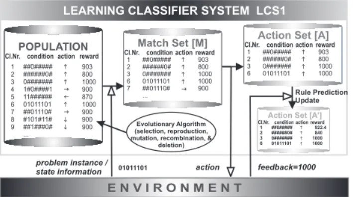
LEARNING CLASSIFIER SYSTEM LCS1 POPULATION condition ##0##### ######0# 0####### 1#0####1 11###### 01011101 ##01110# #101#11# ##1###0# ... action h h h g f h g i i reward 903 800 1000 900 870 1000 900 900 900 Cl.Nr. 1 2 3 4 5 6 7 8 9 problem instance / state information 01011101 condition ##0##### ######0# 0####### 01011101 ##01110# ... action h h h h g reward 903 800 1000 1000 900 Match Set [M] Cl.Nr. 1 2 3 6 7
Action Set [A]
condition ##0##### ######0# 0####### 01011101 ... action h h h h reward 903 800 1000 1000 Cl.Nr. 1 2 3 6 action
Action Set [A’]
condition ##0##### ######0# 0####### 01011101 ... action h h h h reward 922.4 840 1000 1000 Cl.Nr. 1 2 3 6 Rule Prediction Update Evolutionary Algorithm (selection, reproduction, mutation, recombination, &
deletion)
feedback=1000 E N V I R O N M E N T
Figure 1. LCS iteratively interacts and learns from a problem / environment.
matchthe current given problem instance forming amatch
set. The classifiers in the match set essentially specify the
current knowledge of the LCS about the problem instance. Consequently, the match set is used to decide on the clas-sification, action, or prediction, dependent on the problem type and exploration strategy applied. If an action is
cho-sen, anaction set is formed that contains all classifiers in
the match set that specify the chosen action. Once feed-back is available about the decision made, predictions and fitness values of the classifiers in the action set are updated Finally, the evolutionary component is applied. Usually, a steady-state genetic algorithm reproduces some classifiers and deletes others based on the fitness estimates. Figure 1 illustrates the learning process.
Thus, two learning mechanisms are at work. Gradient-based methods generate maximally suitable predictions and derive the fitness measure out of it. Dependent on the fit-ness measure used, classifiers are reproduced that yield high payoff, as done in the ZCS system [34], or also that generate accurate predictions, as done in the XCS system [35]. Thus, since the evolutionary algorithm relies on a fitness estimate generated by the chosen gradient-based method applied, it is essential that the LCS is designed in such a way that the gradient method identifies better classifiers as fast as possi-ble so that the evolutionary component can lead the evolu-tionary process towards a suitable solution representation.
4. Problem Types
Generally, an LCS can be applied to any type of pre-diction problem imaginable. LCSs are designed to evolve solutions by partitioning the problem space into subspaces in which suitable predictions can be formed. Thus, LCSs are designed to detect those problem input features, or in-put subspaces, that are relevant to form effective or accurate predictions. We now discuss three distinct, albeit related,
problem types and the problem solution representation that an LCS would typically evolve in such a problem.
Classification Problems A classification problem is
typ-ically defined over a set of problem instances that consists of a set of features and a corresponding problem class. For example, in datamining, we intend to analyze datasets that contain various problem instances.
For example, the UCI repository [4] contains a mush-room dataset. Each instance in the dataset describes prop-erties of a particular mushroom and partitions the mush-rooms into edible and poisonous ones. The task for an LCS would then be to learn to be able to decide if a mushroom, given its properties, is edible or not. Classification prob-lems can have various input features, such as nominal ones, real-valued ones, and binary ones and they may also contain more than two problem classes.
Comparisons of various LCSs with standard machine learning techniques have shown that the classification qual-ity is comparable to those of state-of-the art machine learn-ing techniques [2, 3, 8]. Also binary classification prob-lems, such as the well-studied multiplexer problem [8, 35, 36], are part of this problem class.
Reinforcement Learning Problems Besides
classifica-tion problems, LCSs have been successfully applied to be-havioral policy learning problems, typically describable by a Markov decision process [30]. In RL problems, feedback is provided only in the form of reward values, which needs to be propagated over the problem space to be able to decide on a proper action to execute. Thus, LCSs learn to propa-gate reward and evolve those classifiers that either predict the reward accurately or that predict the correct action ac-curately. While classification problems are usually single-step problems in which the successive problem inputs are independent of each other, in RL problems successive in-stances typically depend on each other and a solution can
only be found if reward ispropagatedthroughout the
prob-lem space.
A typical example of an RL problem is a path finding problem in a maze, in which reward is only provided at cer-tain goal locations and the learning algorithm has to find the shortest path to the goal (or the closest goal) from all posi-tions in the maze. LCS systems, and in particular the XCS classifier system, have shown robust performance in various maze tasks [11] but also in the mountain car problem [25] and blocks world problems [8, 10].
Function Approximation Problems Besides
classifica-tion and RL problems, another class of problems can be de-scribed as function approximation problems. In these prob-lems, the LCS learns the underlying function of a particu-lar problem. That is, given certain input values, the LCS
predicts the output value(s). Often, LCSs evolve overlap-ping, piecewise linear function value approximations, as is the case for the XCS system [37, 7].
The wide variety of problems above suggests that there are multiple domains of potential applications of LCSs. We now proceed to specify the general structure of the XCS classifier system, its learning approach, and its solution rep-resentation.
5. The XCS Classifier System
The XCS classifier system [35, 36] is an LCS that evolves its classifiers by an accuracy-based fitness ap-proach. XCS has been successfully applied to various prob-lem types and may be the most widely used classifier system today. We now first give an overview over the system and next highlight some of the major successful applications.
5.1. XCS in a Nutshell
XCS’s main differences to earlier LCS systems are (1) its accuracy-based fitness approach and (2) its niche based reproduction process. To accomplish this, several modifi-cations in classifier representation and GA application were necessary.
Knowledge Representation As other LCSs, XCS
repre-sents its knowledge by a population of classifiers. The pop-ulation size in XCS is usually set to a fixed upper bound. Each classifier contains the usual condition, action, and re-ward prediction parts. Additionally, though, each classifier contains a prediction error estimate and a fitness estimate, which reflects the accuracy (inverse error) of a classifier rel-ative to overlapping, competing classifiers. Thus, fitness represents the relative accuracy of a classifier with respect to current competing classifiers (those in common match or action sets).
Evolutionary Component Consequently, the
evolution-ary component propagates classifiers with more accu-rate prediction values. Since the evolutionary component evolves classifier structure (condition and action parts), structures evolve that allow the generation of maximally accurate predictions. Dependent on the problem and the condition representation used, the problem space is conse-quently clustered for the generation of accurate predictions.
Unlike population-wide reproduction and deletion in
previous LCSs, XCS reproduces in the current match or ac-tion set while it continuous to delete classifiers in the whole population. Thus, the evolutionary component searches in the current problem niche, defined by the given problem instance, for better problem sub-solutions, based on the
matching classifiers. In this way, evolution searches more locally in problem subspaces. Moreover, since deletion still takes place in the whole population, an intrinsic general-ization pressure applies because the average classifier con-dition in the match set covers on average a larger problem subspace than the average classifier condition in the pop-ulation, so that (without additional fitness influence) more general classifiers will be reproduced and less general clas-sifiers will be deleted.
This combination leads to the desired learning process that generates maximally accurate and maximally general classifiers. Consequently, the solution representation as a whole becomes maximally accurate and maximally general and is represented by partially overlapping classifiers [12, 13, 8].
5.2. Capabilities
After highlighting the novel features of the XCS clas-sifier system, we now proceed to give an overview over the major system capabilities. We essentially highlight that XCS, in its various forms, can accurately solve large, chal-lenging classification problems, RL problems, as well as function approximation problems.
Classification Various studies have shown that XCS can
solve very large and noisy classification problems. Maybe the most common test function in the LCS literature is the multiplexer problem [34, 35]. It has been show that XCS is able to even solve the highly challenging 70-bit multi-plexer [13]. To solve the problem successfully, it requires a
population size of at least20kclassifiers and about3
mil-lion learning iterations [8]. With population sizes less than
N = 20k, performance sometimes does not reach
com-plete accuracy but gets stuck in a sub-optimal, overgeneral solution representation. Bounding models that determine a minimum population size to ensure successful learning with high probability can be found elsewhere (cf. [8] and references therein). Besides the successful solution of the multiplexer problem and other binary classification prob-lems, XCS has also been applied to datamining problems. In these cases, several studies have shown that XCS per-forms machine-learning competitively, that is, it classifies data similarly well when compared to other machine learn-ing techniques [2, 3, 8].
Reinforcement Learning Besides classification
prob-lems, XCS has been applied successfully to various rein-forcement learning problems. Particularly, various maze tasks have been studied including mazes with discrete and continuous representations as well as mazes that require the formation of long reward chains. Hereby, it is important to use a stabilization component in the gradient-based update
to ensure learning success [11]. In discrete domains, it has been shown that XCS is particularly noise robust as well as very efficient to identify prediction-relevant parameters eas-ily handling (and efficiently identifying and consequently ignoring) even 90 irrelevant additional, randomly fluctuat-ing binary input features [8]. Most recently, XCS for con-tinuous inputs has been shown to be able to also solve the Mountain car problem [25] effectively.
Function Approximation In the above applications,
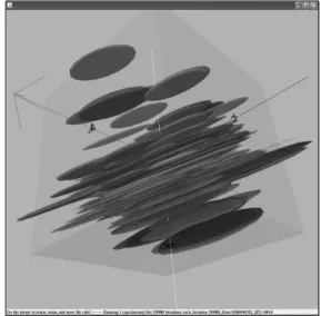
XCS mostly learned constant prediction values. Recently, though, this representation has been expanded to linear rep-resentations and others [24, 25, 37]. In function approx-imation problems, XCSF (the ’F’ stands for function ap-proximation) has been shown to solve various challeng-ing functions includchalleng-ing superimposed sine and ridge func-tions with partially overlapping linear approximators. Re-cent investigations [14] have shown that XCSF outperforms self-organizing map approaches, such as the NeuralGAS algorithm [27], and performs comparably to statistical lo-cal learning approaches, such as constructive incremental learning by Schaal and Atkeson [29]. Meanwhile, however, XCS is a much more general learning approach that can be applied to more problems than those suitable for Neu-ralGAS nets or the constructive incremental learning ap-proach. With respect to scalability, it has been shown that XCS can handle even seven dimensional real-valued input spaces, developing, for example, an accurate approximation surface for the oblique sinusoidal functionf(x1, ..., x7) = sin(4π(x1+...+x7)).
XCSF is now also available online as a Java implemen-tation [9]. Figure 2 shows a screenshot of a typical final problem solution representation of XCSF in the specified oblique sinusoidal sine function in a three dimensional in-put space. It can be seen that XCSF detects the oblique ori-entation of the sine function and consequently partitions the problem space along the axis (0,0,0) to (1,1,1) to be able to form maximally accurate linear predictions with maximally general classifier conditions. Note that the representation scales the condition sizes down in order to make the space partitioning observable.
6. Conclusions
This LCS introduction has provided a glimpse at the functioning and current capabilities of LCSs and the XCS classifier system in particular. LCS form problem solu-tions represented by partially overlapping subsolusolu-tions. It learns such solutions by a combination of gradient-based subsolution approximation and evolutionary-based subso-lution structuring. More recent LCS research has begun to understand the dynamics of the systems sufficiently well, generating scalable and robust LCSs.
Figure 2. Representation of the conditions of a typical, final, accurate classifier population in a three dimensional oblique sine function.
In comparison to other machine learning techniques, per-formance has been shown to be competitive and sometimes even superior. While being competitive, the LCS technique is much more broadly applicable than the systems compared with. Current research focuses on the optimization of clas-sifier operators, further application studies, and more de-tailed rigorous system analysis. What remains to be shown is in which problem types the flexibility of the evolutionary algorithm in combination with efficient gradient-based ap-proximation techniques is superior to other machine learn-ing techniques. It seems that this will be particularly the case in problem domains in which either many local minima prevent other local, distributed gradient-based techniques to fail or in which gradient-based techniques cannot be applied at all since the gradient information can not be used directly to structure the problem space.
References
[1] J. Bacardit. Pittsburgh Genetic-Based Machine Learning in the Dame Mining Era: Representations, Generalization,
and Run Time. PhD thesis, Computer Engineering
Depart-ment, University of Ramon Llull, Barcelona, Spain, 2004. [2] E. Bernad´o, X. Llor`a, and J. M. Garrell. XCS and GALE:
A comparative study of two learning classifier systems and six other learning algorithms on classification tasks. In P. L. Lanzi, W. Stolzmann, and S. W. Wilson, editors,Advances
in Learning Classifier Systems (LNAI 2321), pages 115–132.
Springer-Verlag, Berlin Heidelberg, 2002.
[3] E. Bernad´o-Mansilla and J. M. Garrell-Guiu. Accuracy-based learning classifier systems: Models, analysis, and
ap-plications to classification tasks.Evolutionary Computation, 11:209–238, 2003.
[4] C. Blake, E. Keogh, and C. Merz. UCI repos-itory of machine learning databases, 1998. (http://www.ics.uci.edu/mlearn/MLRepository.html). [5] L. B. Booker. Intelligent Behavior as an Adaptation to the
Task Environment. PhD thesis, The University of Michigan,
1982.
[6] L. B. Booker. Classifier systems that learn internal world models.Machine Learning, 3:161–192, 1988.
[7] M. V. Butz. Kernel-based, ellipsoidal conditions in the real-valued XCS classifier system. GECCO 2005: Genetic and
Evolutionary Computation Conference, pages 1835–1842,
2005.
[8] M. V. Butz. Rule-Based Evolutionary Online Learning
Sys-tems: A Principled Approach to LCS Analysis and Design.
Springer-Verlag, Berlin Heidelberg, 2006.
[9] M. V. Butz. Documentation of XCSFJava 1.1 plus visual-ization. MEDAL Report 2007008, Missouri Estimation of Distribution Algorithms Laboratory, University of Missouri in St. Louis, MO, 2007.
[10] M. V. Butz and D. E. Goldberg. Generalized state val-ues in an anticipatory learning classifier system. In M. V. Butz, O. Sigaud, and P. G´erard, editors,Anticipatory Behav-ior in Adaptive Learning Systems: Foundations, Theories,
and Systems, pages 282–301. Springer-Verlag, Berlin
Hei-delberg, 2003.
[11] M. V. Butz, D. E. Goldberg, and P. L. Lanzi. Gradient descent methods in learning classifier systems: Improving XCS performance in multistep problems. IEEE
Transac-tions on Evolutionary Computation, 9:452– 473, 2005.
[12] M. V. Butz, D. E. Goldberg, and K. Tharakunnel. Analysis and improvement of fitness exploitation in XCS: Bounding models, tournament selection, and bilateral accuracy.
Evo-lutionary Computation, 11:239–277, 2003.
[13] M. V. Butz, T. Kovacs, P. L. Lanzi, and S. W. Wilson. To-ward a theory of generalization and learning in XCS.IEEE
Transactions on Evolutionary Computation, 8:28–46, 2004.
[14] M. V. Butz, P. L. Lanzi, and S. W. Wilson. Function ap-proximation with XCS: Hyperellipsoidal conditions, recur-sive least squares, and compaction. IEEE Transactions on
Evolutionary Computation, in press.
[15] K. A. DeJong, W. M. Spears, and D. F. Gordon. Using ge-netic algorithms for concept learning. Machine Learning, 13(2/3):161–188, 1993.
[16] D. E. Goldberg. Computer-aided gas pipeline operation us-ing genetic algorithms and rule learnus-ing. Dissertation
Ab-stracts International, 44(10):3174B, 1983. Doctoral
disser-tation, University of Michigan.
[17] D. E. Goldberg. Genetic Algorithms in Search,
Optimiza-tion and Machine Learning. Addison-Wesley, Reading, MA,
1989.
[18] J. H. Holland.Adaptation in Natural and Artificial Systems. University of Michigan Press, Ann Arbor, MI, 1975. second edition, 1992.
[19] J. H. Holland. Adaptation. In R. Rosen and F. Snell, editors,
Progress in theoretical biology, volume 4, pages 263–293.
Academic Press, New York, 1976.
[20] J. H. Holland. Properties of the bucket brigade algorithm.
Proceedings of an International Conference on Genetic
Al-gorithms and their Applications, pages 1–7, 1985.
[21] J. H. Holland and J. S. Reitman. Cognitive systems based on adaptive algorithms. In D. A. Waterman and F. Hayes-Roth, editors,Pattern directed inference systems, pages 313–329. Academic Press, New York, 1978.
[22] T. Kovacs. Strength or Accuracy: Credit Assignment in
Learning Classifier Systems. Springer-Verlag, Berlin
Hei-delberg, 2003.
[23] P. L. Lanzi. An analysis of generalization in the XCS clas-sifier system. Evolutionary Computation, 7(2):125–149, 1999.
[24] P. L. Lanzi, D. Loiacono, S. W. Wilson, and D. E. Goldberg. Extending XCSF beyond linear approximation. GECCO
2005: Genetic and Evolutionary Computation Conference,
pages 1827–1834, 2005.
[25] P. L. Lanzi, D. Loiacono, S. W. Wilson, and D. E. Goldberg. Classifier prediction based on tile coding. GECCO 2006:
Genetic and Evolutionary Computation Conference, pages
1497–1504, 2006.
[26] X. Llor`a and J. M. Garrell. Knowledge independent data mining with fine-grained parallel evolutionary algorithms.
Proceedings of the Third Genetic and Evolutionary
Compu-tation Conference (GECCO-2001), pages 461–468, 2001.
[27] T. M. Martinetz, S. G. Berkovitsch, and K. J. Schulten. ”Neural-gas” network for vector quantization and its appli-cation to time-series prediction.IEEE Transactions on
Neu-ral Networks, 4:558–569, 1993.
[28] I. Rechenberg. Evolutionsstrategie Optimierung
technis-cher Systeme nach Prinzipien der biologischen Evolution.
Friedrich Frommann Verlag, Stuttgart-Bad Cannstatt, 1973. [29] S. Schaal and C. G. Atkeson. Constructive incremental learning from only local information.Neural Computation, 10:2047–2084, 1998.
[30] R. S. Sutton and A. G. Barto. Reinforcement learning: An
introduction. MIT Press, Cambridge, MA, 1998.
[31] C. J. C. H. Watkins. Learning from Delayed Rewards. PhD thesis, King’s College, Cambridge, UK, 1989.
[32] S. W. Wilson. Knowledge growth in an artificial animal.
Proceedings of an International Conference on Genetic
Al-gorithms and Their Applications, pages 16–23, 1985.
[33] S. W. Wilson. Classifier systems and the animat problem.
Machine Learning, 2:199–228, 1987.
[34] S. W. Wilson. ZCS: A zeroth level classifier system.
Evolu-tionary Computation, 2:1–18, 1994.
[35] S. W. Wilson. Classifier fitness based on accuracy.
Evolu-tionary Computation, 3(2):149–175, 1995.
[36] S. W. Wilson. Generalization in the XCS classifier system.
Genetic Programming 1998: Proceedings of the Third
An-nual Conference, pages 665–674, 1998.
[37] S. W. Wilson. Classifiers that approximate functions.
Natu-ral Computing, 1:211–234, 2002.
[38] S. W. Wilson and D. E. Goldberg. A critical review of clas-sifier systems.Proceedings of the Third International