Knowledge extraction from
biomedical data using machine
learning
Nicola Lazzarini
Submitted for the degree of Doctor of
Philosophy in the School of Computing
Science, Newcastle University
June 2017
I declare that this thesis is my own work unless otherwise stated. No part of this thesis has previously been submitted for a degree or any other qualification at Newcastle University or any other institution.
Date...
“
world that wasn’t in the world before. It doesn’t matter what it is. It doesn’t matter if it’s a table or a film or gardening - everyone should create. You should do something, then sit back and say: “I did that.”
”
Thanks to the breakthroughs in biotechnologies that have occurred during the recent years, biomedical data is accumulating at a previously unseen pace. In the field of biomedicine, decades-old statistical methods are still commonly used to analyse such data. However, the simplicity of these approaches often limits the amount of useful information that can be extracted from the data. Machine learning methods represent an important alternative due to their ability to capture complex patterns, within the data, likely missed by simpler methods.
This thesis focuses on the extraction of useful knowledge from biomedical data using machine learning. Within the biomedical context, the vast majority of machine learn-ing applications focus their e↵ort on the generation and validation of prediction models. Rarely the inferred models are used to discover meaningful biomedical knowledge. The work presented in this thesis goes beyond this scenario and devises new methodologies to mine machine learning models for the extraction of useful knowledge.
The thesis targets two important and challenging biomedical analytic tasks: (1) the inference of biological networks and (2) the discovery of biomarkers. The first task aims to identify associations between di↵erent biological entities, while the second one tries to discover sets of variables that are relevant for specific biomedical conditions. Successful solutions for both problems rely on the ability to recognise complex inter-actions within the data, hence the use of multivariate machine learning methods. The network inference problem is addressed with FuNeL: a protocol to generate networks based on the analysis of rule-based machine learning models. The second task, the biomarker discovery, is studied with RGIFE, a heuristic that exploits the information extracted from machine learning models to guide its search for minimal subsets of variables.
The extensive analysis conducted for this dissertation shows that the networks inferred with FuNeL capture relevant knowledge complementary to that extracted by standard inference methods. Furthermore, the associations defined by FuNeL are discovered
data, RGIFE confirmed the importance of previously identified biomarkers, whilst also extracting novel biomarkers with possible future clinical applications.
Overall, the thesis shows new e↵ective methods to leverage the information, often remaining buried, encapsulated within machine learning models and discover useful biomedical knowledge.
Part of the work within this thesis have been documented in the following publications:
J. Bacardit, P. Widera,N. Lazzarini, and N. Krasnogor. “Hard data analytics prob-lems make for better data analysis algorithms: bioinformatics as an example”Big data, vol. 2, no. 3, pp. 164-176, sep 2014.
F Eduati et. al. “Prediction of human population responses to toxic compounds by a collaborative competition”. Nature Biotechnology, vol. 33, pp. 933-940, aug 2015.
N. Lazzarini, P. Widera, S. Williamson, R. Heer, N. Krasnogor, and J. Bacardit. “Functional networks inference from rule-based machine learning models” BioData
Mining, vol. 9, sep 2016.
S. Baron, N. Lazzarini and J. Bacardit. “Characterising the influence of rule-based knowledge representations in biological knowledge extraction from transcriptomics data”EvoBio 2017, Evolutionary Computation, Machine Learning and Data Mining for Biology and Medicine, in press, apr 2017.
N. Lazzariniand J. Bacardit. “RGIFE: a ranked guided iterative feature elimination heuristic for the identification of biomarkers”BMC Bioinformatics, in press 2017.
Under review:
N. Lazzarini, J. Runhaar, A.C. Bay-Jensen, C.S. Thudium, S.M.A. Bierma-Zeinstra, Y.Henrotin and J. Bacardit. “A machine learning approach for the identification of reduced panels of biomarkers and its application to knee osteoarthritis incidence in overweight and obese women”Osteoarthritis and Cartilage
First and foremost I wish to thank my supervisors, Dr. Jaume Bacardit and Prof. Natalio Krasnogor for giving me the chance to pursue a Ph.D. at Newcastle University. Your advice and guidance during these years have been truly invaluable and helped me in enhancing the quality of my work.
A special thank goes to Dr. Pawel Widera. Your support has been fundamental during my Ph.D. adventure since the first day. All your help, advice and suggestions made me a better scientist.
I would also like to thank all the colleagues from the ICOS (Interdisciplinary Comput-ing and Complex BioSystems) research group. I am grateful to the people in 922 that had to hear me ranting and complaining during the last four years. They helped me to see the brighter side of things and always gave me hope. I was lucky to complete my Ph.D. together with supporting people, especially Dr. Jurek Kozyra, Dr. Annunziata Lopiccolo and Dr. G¨oksel Misirli. Finally, I need to mention Fedor Shmarov, Jens Geyti and Dr. Joseph Mullen that made my Ph.D. experience a bit lighter.
I wish to thank the School of Computing Science and Newcastle University. Also, the Engineering and Physical Sciences Research Council (EPSRC) that supported my work [EP/L001489/2, EP/J004111/2, EP/I031642/2, EP/N031962/1]. Furthermore, I am thankful to the European Union Seventh Framework Programme (FP7/2007-2013) that funded part of this work under the “D-BOARD” project (grant agreement number 305815). I am also thankful to my examiners Prof. John H. Holmes and Prof. Anil Wipat for their time dedicated to my dissertation and for the valuable feedback received.
Last but not least, a very special thanks must go to my parents and my brother. Your continuous support and encouragement helped me towards my whole decennial academic path until the finish line. Thank you.
1 Introduction 21
1.1 Background and motivation . . . 22
1.2 Overview of the problem . . . 24
1.3 Aims and scope . . . 26
1.4 Thesis Structure . . . 28
1.5 Main contributions . . . 29
2 Background Research 30 2.1 Types of biological data . . . 31
2.2 Introduction to machine learning . . . 33
2.2.1 Machine learning paradigms . . . 33
2.2.2 Supervised learning . . . 35
2.2.2.1 The classification problem . . . 35
2.2.2.2 The knowledge representation in supervised learning . 40 2.2.3 Unsupervised learning . . . 47
2.3 Machine learning for the inference of biological networks . . . 50
2.4 Similarity-based approaches for the inference of biological networks . . 53
2.4.1 Correlation-based methods . . . 54
2.4.2 Mutual information-based methods . . . 55
2.5 Network inference via the integration of multiple data . . . 56
2.6 Statistical approaches for biomarkers identification . . . 57
2.7 Machine learning for biomarkers identification . . . 61
2.8 Knowledge integration in machine learning methods for biomarkers identification . . . 63
2.9 Biomedical evaluation of the results . . . 64
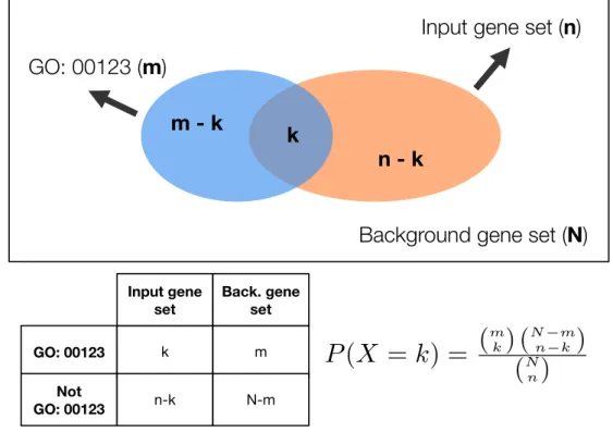
2.9.1 Enrichment analysis . . . 65
2.9.2 Gene-disease associations . . . 69
3.1 Introduction . . . 73
3.2 Material and Methods . . . 77
3.2.1 The co-prediction paradigm . . . 77
3.2.2 The FuNeL protocol . . . 79
3.2.3 Datasets . . . 83
3.2.4 Co-expression networks . . . 84
3.2.5 Enrichment analysis . . . 86
3.2.6 Disease association analysis . . . 86
3.3 Results . . . 87
3.3.1 Identification of predefined relationships in synthetic datasets . 88 3.3.2 Topological comparison of the inferred networks . . . 89
3.3.3 Complementarity of enriched terms . . . 93
3.3.4 Quantifying the amount of captured biological knowledge . . . . 99
3.3.5 Evaluation of the networks in a disease context . . . 101
3.3.6 Prostate cancer case study: enriched terms . . . 103
3.3.7 Prostate cancer case study: disease associations . . . 110
3.4 Discussion . . . 113
3.5 Future work . . . 116
4 RGIFE: a ranked guided iterative feature elimination heuristic for biomarkers identification 118 4.1 Introduction . . . 119
4.2 Material and Methods . . . 123
4.2.1 The RGIFE heuristic . . . 123
4.2.1.1 Relative block size . . . 127
4.2.1.2 Parameters of the classifier . . . 127
4.2.1.3 RGIFE policies . . . 128
4.2.2 Benchmarking algorithms . . . 128
4.2.3 Datasets . . . 130
4.2.4 Experimental design . . . 132
4.2.4.1 Relevant features identification . . . 132
4.2.4.2 Predictive performance validation . . . 133
4.2.4.3 Biomedical relevance analysis of the signatures . . . . 134
4.3.3 Identification of relevant attributes in synthetic datasets . . . . 142
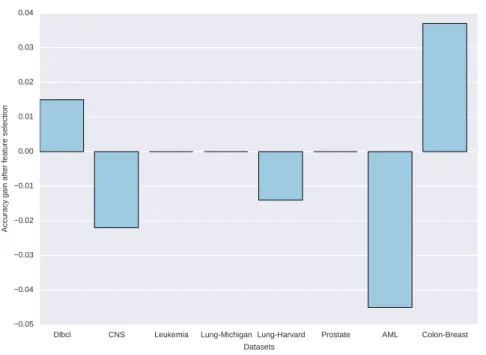
4.3.4 Comparison of the predictive performance with other feature selection methods . . . 145
4.3.5 Analysis of the signatures size . . . 147
4.3.6 Biomedical relevance of the signatures . . . 147
4.4 Discussion . . . 155
4.5 Future work . . . 160
5 Identification of biomarkers for knee osteoarthritis 163 5.1 Introduction . . . 164
5.2 Material and methods . . . 167
5.2.1 Datasets and individuals . . . 167
5.2.2 Extension of RGIFE to analyse the PROOF study data . . . 170
5.2.3 Discovery and evaluation of small sets of biomarkers . . . 172
5.2.3.1 Generation and selection of reduced predictive models using RGIFE . . . 173
5.2.3.2 Permutation tests . . . 175
5.2.3.3 Variable importance . . . 176
5.2.3.4 Variable direction . . . 176
5.2.3.5 Inference of functional networks with FuNeL . . . 177
5.3 Results . . . 178
5.3.1 2.5 years predictive models . . . 178
5.3.1.1 Additive values of the biomarkers . . . 181
5.3.1.2 Biomarkers association with knee OA . . . 184
5.3.1.3 Comparison with literature findings . . . 190
5.3.2 6.5 years predictive models . . . 193
5.3.2.1 Selected models from TNO data . . . 194
5.3.2.2 Additive values of the biomarkers from TNO data . . . 197
5.3.2.3 Biomarkers association with knee OA from TNO data 199 5.3.2.4 Functional networks from TNO data . . . 202
5.3.2.5 Selected models from UNOTT data . . . 204
5.3.2.6 Merging TNO and UNOTT data . . . 206
5.4 Discussion . . . 207
6.2 Evaluation of the research question . . . 217
6.3 Contribution to the area of bio-data mining . . . 219
6.4 Limitations . . . 220
6.4.1 Computational time . . . 221
6.4.2 Co-prediction paradigm . . . 221
6.4.3 Data pre-processing . . . 222
6.4.4 Lack of ground truth and field limitations . . . 222
6.5 Future work . . . 223
6.5.1 Integration of FuNeL and RGIFE . . . 223
6.5.2 Knowledge integration for a better learning . . . 224
6.5.3 Exploring the role of di↵erent knowledge representations . . . . 225
6.5.4 Application to other fields . . . 226
A Appendix 227 A.1 Enrichment score analysis . . . 228
A.2 Disease association analysis . . . 229
A.3 Case study: prostate cancer dataset . . . 232
A.3.1 Overlap of networks enriched terms . . . 232
A.3.2 Genomic alteration in independent dataset . . . 235
A.4 Time complexity analysis . . . 238
B Appendix 240 B.1 Predictive performance with synthetic datasets . . . 241
B.2 Signatures analysed in the case study . . . 242
B.3 Time complexity analysis . . . 244
C Appendix 246 C.1 PROOF study information . . . 247
C.2 Lipidomics functional networks . . . 252
1.1 Example of machine learning applications in bioinformatics . . . 23
1.2 DIKW pyramid model . . . 27
1.3 Knowledge extraction from machine learning models . . . 27
2.1 The central dogma of molecular biology . . . 32
2.2 Illustration of the classification problem . . . 36
2.3 Validation of a predictive model . . . 36
2.4 Example of a ROC curve . . . 39
2.5 Example of a decision tree . . . 41
2.6 Example of a classification rule set . . . 42
2.7 Representation of a classifier using ALKR . . . 43
2.8 Example of linear models . . . 46
2.9 Example of clustering . . . 49
2.10 Example of a PCA plot . . . 50
2.11 The co-expression paradigm . . . 53
2.12 Comparison of PCC and MIC association measures . . . 56
2.13 Taxonomy of feature selection methods . . . 62
2.14 Example of enrichment analysis . . . 66
2.15 Last update of common enrichment tools . . . 69
2.16 The knowledge extraction process from machine learning models . . . . 71
3.1 Comparison of similarity-based and machine learning-based approaches 75 3.2 The FuNeL protocol . . . 76
3.3 The co-prediction paradigm . . . 78
3.4 Changes in accuracy when using SVM-RFE . . . 81
3.5 Example of a BioHEL classification rule set. . . 81
3.6 FuNeL networks generated from the Dlbcl dataset . . . 90
3.7 FuNeL networks generated from the Lung-Michigan dataset. . . 91
3.8 Pearson networks generated from the Lung-Michigan dataset . . . 94
3.9 ARACNE networks generated from the Lung-Michigan dataset . . . 94
3.10 MIC networks generated from the Lung-Michigan dataset . . . 95
3.14 Hubs GO terms comparison between FuNeL and ARACNE networks . 108
3.15 Hubs GO terms comparison between FuNeL and MIC networks . . . . 109
3.16 GO terms overlap between the best (G-D association) FuNeL and co-expression networks . . . 110
3.17 Genomic alteration in independent dataset . . . 112
4.1 Data accumulation at EMBL-EBI . . . 120
4.2 The iterative nature of the RGIFE heuristic and its overall behaviour. 126 4.3 Accuracy comparison for di↵erent RGIFE policies . . . 137
4.4 Number of selected attributes by di↵erent RGIFE policies . . . 139
4.5 Execution time of the original and the new RGIFE . . . 140
4.6 RGIFE iterative process output . . . 141
4.7 Number of selected attributes by di↵erent methods . . . 148
4.8 Analysis of the signatures in a disease-context. . . 149
4.9 Normalised genomic alteration of the signatures in independent data . . 151
4.10 Signature induced network . . . 153
4.11 ClueGO enrichment analysis of the signature induced network . . . 154
5.1 Pipeline for the identification, validation and interpretation of biomarkers173 5.2 Pipeline for the best predictive model selection . . . 174
5.3 ROC curves of the selected models from the 2.5 years data . . . 180
5.4 Variable importance for the ACR criteria model (2.5 years) . . . 182
5.5 Variable importance for the knee pain model (2.5 years) . . . 182
5.6 Variable importance for the lateral JSN model (2.5 years) . . . 183
5.7 Variable importance for the medial JSN model (2.5 years) . . . 184
5.8 Variable importance for the K&L score incidence model (2.5 years) . . 185
5.9 Variable direction for the ACR criteria model (2.5 years) . . . 186
5.10 Variable direction for the knee pain model (2.5 years) . . . 187
5.11 Variable direction for the lateral JSN model (2.5 years) . . . 188
5.12 Variable direction for the medial JSN model (2.5 years) . . . 190
5.13 Variable direction for the K&L score incidence model (2.5 years) . . . . 191
5.14 ROC curves of the selected models from the 6.5 years data . . . 195
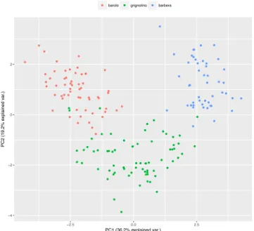
5.15 PCA plot from the ACR criteria biomarkers . . . 196
5.19 Variable direction for the ACR criteria model (6.5 years) . . . 199 5.20 Variable direction for the knee pain model (6.5 years) . . . 200 5.21 Variable direction for the K&L score incidence model (6.5 years) . . . . 201 5.22 The main clusters of the FuNeL networks . . . 205
A.1 Unique GO terms from FuNeL and ARACNE networks . . . 233 A.2 Unique GO terms from FuNeL and MIC networks . . . 234 A.3 Genomic alterations of FuNeL network hubs in independent data . . . . 235 A.4 Genomic alterations of FuNeL network central nodes in independent data236 A.5 Genomic alterations of Pearson network hubs in independent data . . . 236 A.6 Genomic alterations of Pearson network central nodes in independent
data . . . 236 A.7 Genomic alterations of ARACNE network hubs in independent data . . 237 A.8 Genomic alterations of ARACNE network central nodes in
independent data . . . 237 A.9 Genomic alterations of MIC network hubs in independent data . . . 237 A.10 Genomic alterations of MIC network central nodes in independent data 238 A.11 BioHEL execution time . . . 239
B.1 Average execution times of each method across di↵erent datasets . . . . 244
C.1 FuNeL network generated using the ACR criteria data (6.5 years) . . . 253 C.2 FuNeL network generated using the knee pain data (6.5 years) . . . 254 C.3 FuNeL network generated using the KL score incidence data (6.5 years) 255
2.1 Example of a confusion matrix . . . 37
3.1 Description of the FuNeL configurations . . . 82
3.2 Description of the datasets used to infer networks . . . 84
3.3 FuNeL success rate in the identification of disease-predicting SNPs. . . 88
3.4 Topological properties of FuNeL and Pearson co-expression networks. . 91
3.5 Topological properties of FuNeL and ARACNE co-expression networks. 92 3.6 Topological properties of FuNeL and MIC co-expression networks. . . 93
3.7 Enriched GO terms overlap between FuNeL configurations . . . 95
3.8 Enriched GO terms overlap between FuNeL and co-expression networks 96 3.9 Enriched GO terms di↵erence between FuNeL and random networks . . 97
3.10 Enriched pathways di↵erence between FuNeL and random networks . . 98
3.11 Enriched GO terms overlap between FuNeL and random networks. . . . 98
3.12 Enriched pathways overlap between FuNeL and random networks. . . . 98
3.13 Average (best) networks ranks based on the Enrichment Score . . . 100
3.14 Average networks ranks based on the Enrichment Score . . . 101
3.15 Average (best) networks ranks based on the G-D associations . . . 102
3.16 Average networks ranks based on the G-D associations (curated) . . . . 103
3.17 Average networks ranks based on the G-D associations (Malacards) . . 103
3.18 Unique and common terms from networks’ hubs . . . 106
3.19 Average genomic alterations in independent dataset . . . 113
4.1 Description of the synthetic datasets used in the experiments . . . 131
4.2 Description of the real-world datasets used in the experiments. . . 132
4.3 Average performance ranks for di↵erent RGIFE policies . . . 137
4.4 Comparison of BioHEL and random forest classification accuracy . . . 138
4.5 Average Success Index on synthetic datasets . . . 143
4.6 Summary of the analysis on the SD datasets . . . 143
4.7 Summary of the analysis on the madsim datasets . . . 145
4.8 Accuracy comparison for di↵erent methods . . . 146
4.9 EnrichNet analysis of the signature induced network . . . 155
5.4 Summary of the models inferred from the 2.5 years data . . . 179
5.5 Summary of the K&L score incidence models found in the specialised literature . . . 192
5.6 Summary of the knee pain models found in the specialised literature . . 193
5.7 Summary of the models inferred from the 6.5 years data . . . 194
5.8 Topological properties of the lipidomics functional networks . . . 202
5.9 Role of the RGIFE selected lipids within the FuNeL networks. . . 203
5.10 Summary of the inferred models from the 6.5 years data (TNO+UNOTT) . . . 207
A.1 ES based ranks for FuNeL networks . . . 228
A.2 ES based ranks for Pearson networks . . . 228
A.3 ES based ranks for ARACNE networks . . . 228
A.4 ES based ranks for MIC networks . . . 229
A.5 Malacards G-D based ranks for FuNeL networks . . . 229
A.6 Malacards G-D based ranks for Pearson networks . . . 230
A.7 Malacards G-D based ranks for ARACNE networks . . . 230
A.8 Malacards G-D based ranks for MIC networks . . . 230
A.9 Curated G-D based ranks for FuNeL networks . . . 231
A.10 Curated G-D based ranks for Pearson networks . . . 231
A.11 Curated G-D based ranks for ARACNE networks . . . 231
A.12 Curated G-D based ranks for MIC networks . . . 231
B.1 Accuracies of di↵erent methods using the synthetic datasets . . . 241
B.2 Accuracies of di↵erent methods using the madsim datasets . . . 242
ACR American College of Rheumatology AUC Area Under the ROC Curve
DB-SCV Distributed Balanced-Stratified Cross Validation G-D Gene-Disease association
GO Gene Ontology
GNB Gaussian Naive Bayes JSN Joint Space Narrowing KL Kellgren & Lawrence KNN K-nearest neighbour
LOOCV Leave One Out Cross Validation MIC Maximal Information Coefficient OA Osteoarthritis
PCA Principal Component Analysis PCC Pearson Correlation Coefficient PPI Protein Protein Interaction SPL Shortest Path Length SVM Support Vector Machine RF Random Forest
1
Introduction
Contents
1.1 Background and motivation . . . 22
1.2 Overview of the problem . . . 24
1.3 Aims and scope . . . 26
1.4 Thesis Structure . . . 28
1.1
Background and motivation
During the last few decades, the advances in high-throughput technologies have led to an explosion in the availability of biomedical data, which subsequently increased the understanding of how those data can be used to improve human life. The analysis of such a large amount of data can help us in revealing and explaining the complex mechanisms that characterise biological and medical conditions. However, this goal can only be achieved if appropriate analytical tools are designed to fully exploit the large quantity of available information and extract relevant knowledge.
Statistical-based and computational methodologies have been extensively applied for data analysis in the field of biomedicine, trying to underline difficult biological and medical processes [1–3]. However, due to the simplicity of these approaches (e.g. lin-ear models or univariate techniques), the amount and the kind of information that can be extracted from the data is limited [4]. Machine learning represents a powerful alternative that can o↵er better, more robust and flexible solutions and is currently rising in the field of biomedicine [5]. The advantageous position of machine learning methods is given by the use of complex multivariate knowledge representations that allow, when mining the data, to discover interesting patterns that are often missed by simpler approaches. Thanks to such a rich and diverse knowledge representation, ma-chine learning approaches are well suited for the analysis of biomedical data that often are characterised by: large dimensionality (high number of variables), class imbalance distribution (e.g. many more healthy patients than sick), vast number of samples, information collected from di↵erent sources (e.g. clinical examination, gene expression levels, protein abundances), etc. Hence, over the years, the use of machine learning methods has proven successful in many di↵erent biosciences: medicine [6], biology [7], chemistry [8], etc.
Machine learning is defined as the set of methods that automatically learn from experi-ence [9]. Machine learning algorithms analyse the data and generate solutions (models) to address a large variety of complex problems. Now, once the model is inferred, if we understand why the algorithm performed certain choices or we interpret the structure of the solutions, we have the possibility to learn something. The experienced gained
by the algorithms when analysing the data can help us in improving the understanding of biomedical questions. For example, the presence of certain features or the relation-ships between specific components of the computational models are information that can reveal new unexpected insights. The challenges in identifying and extract this information provide the primary motivation for this thesis. Inspired by the possibility to gain new interesting and relevant knowledge, novel methodologies are presented for the mining of machine learning models generated from biomedical data.
In addition to all these applications, computa-tional techniques are used to solve other problems, such as efficient primer design for PCR, biological image analysis and backtranslation of proteins (which is, given the degeneration of the genetic code, a complex combinatorial problem).
Machine learning consists in programming computers to optimize a performance criterion by using example data or past experience. The optimized criterion can be the accuracy provided by a predictive model—in a modelling problem—, and the value of a fitness or evaluation function—in an optimization problem.
In amodelling problem, the ‘learning’ term refers to running a computer program to induce a model by using training data or past experience. Machine learning uses statistical theory when building computational models since the objective is to
make inferences from a sample. The two main steps in this process are to induce the model by processing the huge amount of data and to represent the model and making inferences efficiently. It must be noticed that the efficiency of the learning and inference algorithms, as well as their space and time complexity and their transparency and inter-pretability, can be as important as their predictive accuracy. The process of transforming data into knowledge is both iterative and interactive. The iterative phase consists of several steps. In the first step, we need to integrate and merge the different sources of information into only one format. By using data warehouse techniques, the detection and resolution of outliers and inconsistencies are solved. In the second step, it is necessary to select, clean and transform the data. To carry out this step, we need to eliminate or correct the uncorrected data, as well as
Figure 1: Classification of the topics where machine learning methods are applied.
88 Larran‹aga et al.
by guest on August 27, 2016
http://bib.oxfordjournals.org/
Downloaded from
Fig 1.1: Example of the possible applications of machine learning in biomedicine as illustrated in [10].
In biomedicine, machine learning methods have been used to solve many di↵erent tasks [10]. As presented in Figure 1.1, machine learning applications can be useful within diverse domains: gene network inference, microarray analysis, pathways investigation, protein function prediction, phylogenetic tree construction, etc. Among them, this thesis focuses on proposing new methodologies that can tackle two main analytic tasks: (1) the inference of biological networks and (2) the discovery of biomarkers (short for biological markers, that is a measure of a biological state). Both are highly relevant and challenging tasks in the field of biomedicine [11, 12]. Their successful resolution requires the ability to capture and exploit the relationships between the entities of
data. Machine learning, with its rich knowledge representations, can contribute in proposing alternative solutions to what is currently existing.
As a consequence of the growth of public biomedical data, the scientific community has been able to disprove theories and beliefs formulated in the past. For example, in 1941 Beadle and Tatum proposed the “one-gene/one-enzyme/one-function” paradigm [13]. Over the years, with the improvement of technologies and the analysis of relevant data, we learnt how the picture is far more complex. It has been established that biological processes and diseases are rarely caused by a single molecule, but they are instead the result of many interactions between several factors. The complicated mechanisms behind those biological processes and diseases can be modelled by complex networks to facilitate their comprehension. When coupled with large-scale data, networks have been proven to provide a useful conceptual framework. Machine learning, with its ability to discover hidden and relevant patterns, can contribute towards filling the gap created by traditional methods based on simple and sometimes limiting approaches.
The large amount of information associated with biomedical data motivates the other research task tackled in this thesis. Modern high-throughput experiments allow the analysis of the relationships and the properties of many biological entities at once. Therefore, the observations included in the data result defined in a high dimensional space. Unfortunately, a vast abundance of irrelevant and sometimes misleading data is encapsulated within those dimensions. Therefore, there is a need for adequate com-putational approaches to recognise and filter out insignificant information. The iden-tification of factors that are important, and potentially can drive a specific condition or disease, assumes the name of biomarkers discovery. Machine learning methods in this context become important, as they can efficiently mine the data and, taking into account possible dependencies among the variables, discard irrelevant information.
1.2
Overview of the problem
When coming to the use of machine learning in biomedicine, most of the research e↵ort tends to focus exclusively on the core data mining tasks of building and applying mod-els [14]. Typical examples in which machine learning is employed are: classification
problems where the goal is the discrimination of patients that belong to di↵erent cat-egories such as controls vs. cases [15], regression problems where the aim is to predict the values of a continuous variable such as the chemical level of a compound [16], clus-tering problems where di↵erent samples (patients) need to be grouped together based on common characteristics [17], etc. Quite often the success of the proposed solution is purely based on performance metrics such as the classification accuracy (i.e. how many patients can the model correctly classify?). Far less interest and e↵ort have gone into the knowledge discovery and the hypothesis generation from the analysis of the data. In this context, machine learning models are simply treated as a “black box” that, given some data as input provide somehow a “magical” solution as output.
The difficulty in interpreting the machine learning solutions is generating a gap with the bioscience experts and is preventing a wider adoption of machine learning tech-niques. Currently, the proposed methods do not always entirely fulfil the needs and the expectations of the bioscientists. As mentioned earlier, mere “black box” solutions are not enough anymore. For example, an oncologist is not interested in a model that can only slightly outperform his ability in identifying cancer cells. On the contrary, he would be fascinated to discover how the classifier recognises cancer cells and which criteria it uses to discriminate them from healthy cells. Machine learning models, if exploited with appropriate techniques, have the potential to fulfil the expressed needs. Thus, as it is currently a common practice, the usage of machine learning narrowed to solve core data mining tasks (e.g. predict the category of the samples) is limiting the advance in the understanding of many biomedical problems, far more can be achieved.
Besides, generic computational algorithms, including machine learning, not always provide the best solution for biomedical problems. Sometimes they cannot adapt to better address the problem in hand. For example, in biomarker discovery, the number of candidates is crucial as the fewer they are, the more likely is to have them experimen-tally validated. Generic machine learning methods which simply aim to maximise the predictive performance of the candidate sets, regardless their size, are not always the best choice. Thus, in this context, better methods are needed. For instance, an algo-rithm that can trade small drops in predictive performance in favour of a smaller set of biomarker candidates, so that is more likely to have them experimentally tested.
Fur-thermore, many methods, based on specific types of knowledge representation, might be able only to capture a limited kind of information. An intrinsic bias is associated to each knowledge representation [18], this narrows down the overall information that each method can extract. Therefore, flexible approaches that can use di↵erent knowl-edge representations and ideally, can identify the best type based on the data being analysed, can improve the provided solution.
Overall, there is an increasing need for methodologies that are designed to solve biomedical problems and can bridge the gap between the generation of computational models and their interpretability for the gaining of new research insights. The work proposed in this thesis is intended to fill this gap and tackle the mentioned problems.
1.3
Aims and scope
Overall, this dissertation tries to verify the following research hypothesis:
Research hypothesis
Can we extract relevant knowledge from the analysis of machine learning models generated from biomedical data?
To test this research hypothesis, the thesis concentrates on the mining and the analysis of the structure of various machine learning models generated from di↵erent biomedical data. The aim is to move a step further from the inference of computational mod-els and verify whether their structure can be used to discover new knowledge. Using the DIKW (Data, Information, Knowledge, Wisdom) model [19] as a reference, rep-resented in Figure 1.2, a typical application of machine learning methods would stop at the model generation (information). Conversely, the research performed through this dissertation, using biomedical data, explores the output of the model generation step (information) to discover new insights (knowledge) that potentially can help to understand complex biomedical problems better (wisdom).
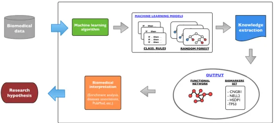
The general process used to extract knowledge from biomedical data is depicted in Figure 1.3. As evident from the figure, the process of exploiting machine learning models can result in di↵erent outputs: from biological networks to the identification
DATA INFORMATION
KNOWLEDGE WISDOM
Fig 1.2: The DIKW (Data, Information, Knowledge, Wisdom) pyramid model.
of biomarkers, from patient stratification to phylogenetic tree inference, etc. For ex-ample, by checking which elements characterise the generated models and how they are used to perform computational tasks, it is possible to deduce if biological entities interact with each other or if they are evolutionarily related. Following the steps illus-trated in Figure 1.3, this dissertation proposes solutions for two important biomedical problems: (1) the inference of biological networks and (2) the identification of small sets of predictive biomarkers. The presented methods aim to: discover relevant knowl-edge and be generic, that is not tailored to handle a specific type of data but instead capable of dealing with a wide variety of biomedical data.
Biomedical data ML algorithm modelML Knowledge extraction Biological networks Phylogenetic trees Patients stratification Network inference Biomarker discovery Patients stratification Phylogenetic tree
Fig 1.3: The process of knowledge extraction through the analysis of machine learning (ML) models generated from biomedical data. In bold are highlighted the research topics on which this thesis is focused.
1.4
Thesis Structure
This thesis is organised into six chapters: the introduction, a preliminary chapter that presents the context and the background material on which the dissertation is built on, three content chapters that describe the contributions of this work to the bio-data mining field and one final chapter that underlines the conclusions and further work. The overall structure of the thesis, excluding this introductory chapter, is the following:
Chapter 2 - Background research introduces the key concepts necessary to un-derstand the content of the dissertation fully. The di↵erent types of biological data are described and is given an introduction to machine learning. This is followed by the presentation of the state-of-the-art approaches employed for (1) the inference of biological networks and (2) the identification of biomarkers. Af-terwards, is included a description of the common approaches employed for the biomedical validation of the knowledge extraction process.
Chapter 3 - FuNeL: a protocol for the inference of functional networks from machine learning modelsdescribes FuNeL, a protocol for the inference of functional networks generated from rule-based machine learning models. The chapter provides an extensive analysis of the networks inferred with FuNeL using both synthetic and real-world data. In addition, FuNeL is contrasted with the state-of-the-art methods for network inference. The comparison is performed from both a biomedical and a topological point of view.
Chapter 4 - RGIFE: a ranked guided iterative feature elimination heuristic for biomarkers identification introduces, improves and evaluates RGIFE: a heuristic for the identification of small sets of biomarkers. The analysis consists of a thorough validation of the new features implemented in the heuristic. Further-more, RGIFE is contrasted with classic methods used for biomarker discovery employing both real-world and synthetic data. The comparison is done in terms of predictive performance and biomedical relevance of the selected biomarkers.
Chapter 5 - Identification of biomarkers for knee osteoarthritis describes the application of machine learning techniques to a variety of biomedical data (from
lipids abundance to clinical measurements) obtained from a knee osteoarthri-tis study. A machine learning-based pipeline, using RGIFE at its core, is used to generate predictive models for the presence of knee osteoarthritis. The pro-posed models are extensively analysed and contrasted with literature findings. In addition, FuNeL is used to infer networks from a subset of the available data.
Chapter 6 - Conclusionssummarises the results and the main findings of the disser-tation. The chapter also includes a discussion of the limitations of the proposed methodologies and possible future work.
1.5
Main contributions
The main contribution of this dissertation is the introduction of new methods for the discovery of relevant knowledge, from machine learning models, for biomedicine. The research performed for this thesis resulted in the:
• definition and evaluation of a protocol, called FuNeL, for the inference of func-tional networks from the analysis of rule-based machine learning models, in Chap-ter 3
• characterisation of a systematic approach to evaluate biological networks based on biomedical knowledge (gene-disease associations), in Chapter 3
• computational improvements and biomedical validation of RGIFE, a heuristic for the identification of small sets of biomarkers guided, in its search for the optimal solutions, by the information extracted from machine learning models, in Chapter 4
• identification of knee osteoarthritis biomarkers via the application of machine learning methods to biomedical data and their characterisation in a network context, in Chapter 5.
2
Background Research
Contents
2.1 Types of biological data . . . 31 2.2 Introduction to machine learning . . . 33 2.2.1 Machine learning paradigms . . . 33 2.2.2 Supervised learning . . . 35 2.2.3 Unsupervised learning . . . 47
2.3 Machine learning for the inference of biological networks . . 50
2.4 Similarity-based approaches for the inference of biological
networks . . . 53 2.4.1 Correlation-based methods . . . 54 2.4.2 Mutual information-based methods . . . 55
2.5 Network inference via the integration of multiple data . . . . 56
2.6 Statistical approaches for biomarkers identification . . . 57 2.7 Machine learning for biomarkers identification . . . 61
2.8 Knowledge integration in machine learning methods for
biomarkers identification . . . 63 2.9 Biomedical evaluation of the results . . . 64 2.9.1 Enrichment analysis . . . 65 2.9.2 Gene-disease associations . . . 69 2.10 Summary . . . 70
Abstract
This chapter introduces the main concepts behind each step of the knowl-edge extraction process employed in this dissertation. The chapter covers the data and the methodologies used to generate both models and hy-pothesis. Afterwards, the approaches available to evaluate the extracted knowledge are presented. More in details, the chapter o↵ers an overview of the type of biological data that can be generated nowadays. In addition, the state-of-the-art approaches for both the inference of biological networks and the discovery biomarkers are described. Finally, the chapter provides an introduction to the methodologies commonly employed to validate the output of the knowledge extraction process in biomedicine.
2.1
Types of biological data
In 1958, Francis Crick proposed a concept that is believed to provide the underpinning of all biology: the central dogma of molecular biology [20]. The dogma describes the flow of genetic information within a biological system. A simplified version of the dogma is illustrated in Figure 2.1. The DNA is transcribed into RNA strands, messenger RNA strands are then translated into proteins that are virtually involved in all the cell functions. Current technologies can provide measurements made on di↵erent tiers of the central dogma and beyond. Those measurements lead to the generation of the so called -omics data. The suffix -omics refers to the collective technologies used to explore the roles, the relationships and the actions of the various types of molecules that make up the cellular activity of an organism.
As suggested in [22], -omics fields can be grouped as:
• Genomics: probably represents the most mature of the di↵erent -omics fields. It is defined as the study of the whole genome sequence (the complete DNA sequence of an organism’s genome) and the information contained therein. A GWAS, also known as Genome Wide Association Study, provides an examina-tion of a genome-wide set of genetic variants in di↵erent individuals to check if any variant is associated with a trait. GWASs mainly focus on the association
DNA
RNA
Proteins
Sugars Nucleotides Amino
acids Lipids Metabolites Genomics Transcriptomics Proteomics Metabolomics Transcription Translation
Fig 2.1: The central dogma of molecular biology and the connections with the type of -omics data obtained from each tier (based on diagram by Lmaps [21]).
between SNPs (Single Nucleotide Polymorphism) and human traits. A SNP is a variation at a single DNA site, they are the most frequent type of variation that can be found in the genome and they have been extensively studied to identify diseases susceptibility and for assessing the efficacy of drug therapies.
• Transcriptomics: contain information about both the presence and the relative abundance of RNA transcripts, by that illustrating the active components within the cell. Microarrays are the most well-established approaches and have been extensively used in many fields of bioinformatics over the years.
• Proteomics: identify and quantify the cellular levels of each protein being en-coded by the genome. Proteomics data can be used for di↵erent purposes such as: biomarkers discovery, analysis of functional pathways and quantification of proteins [23].
• Metabolomics: seek to analyse the set of metabolites (also known as the metabolome) of the cell. The metabolome is the output that results from the cellular integration of the transcriptome and proteome, so it o↵ers both a list
of metabolite components and functional readout of the cellular state. Among the metabolomics data, lipidomics are recently receiving much interest, they have been found to major an important role in many metabolic diseases such as obesity, atherosclerosis, stroke, hypertension and diabetes [24].
The analysis performed for this dissertation involved only the use of transcrip-tomics and lipidomics data. However, the methodologies presented are generic enough to be applied to other types of biological data. Prior to every kind of analysis on -omics data, several pre-processing steps need to be performed (e.g. background correction, normalisation, summarisation, etc.) Di↵erent types of -omics data require di↵erent pre-processing approaches [25]. All the data used for this dissertation were either taken from public repositories or provided by clinicians. In both cases, the data were already pre-processed, so there will be no mention of such techniques in this dissertation.
2.2
Introduction to machine learning
2.2.1
Machine learning paradigms
Many di↵erent definitions have been proposed, over the years, for the term machine learning. In 1959 Arthur Samuel [26] stated that:
“
Machine learning is the subfield of computer science that gives com-puters the ability to learn without being explicitly programmed”
It means that machine learning algorithms are able to perform a specific task without being directly told how to do it. Let’s assume we would like to create a program that can distinguish between spam and valid email messages. We can define a set of rules that highlights the messages that contain certain features such as specific words (e.g. viagra) or explicitly fake adverts. Unfortunately, the generation of an efficient set of rules can be difficult because spammers tend to use strategies to avoid spam filters (e.g vi@gr@ instead of viagra). In this context, machine learning is the solution because, given a set of manually labelled good and bad email examples, an algorithm can automatically learn a set of rules that distinguish them.
Another famous machine learning definition was proposed by Tom Mitchell [9]:
“
Machine Learning as the set of computer algorithms that automati-cally learn from experience”
Following this definition, we can define the learning as:
Definition 2.2.1. A computer program is said to learn from experienceE with respect to some class of tasks T and performance measure P, if its performance at tasks inT, as measured by P, improves with experience E.
According to this definition, we can reformulate the email problem as the task of identifying spam messages (taskT) using the data of previously labelled email messages (experience E) through a machine learning algorithm with the goal of improving the future email spam labelling (measure P).
According to how E, P and T are defined, we can identify di↵erent machine learning paradigms. A classical division of the learning paradigms includes:
• Supervised learningis defined as a learning process where the system is guided (either automatically or by human interaction) and receives feedback about the correctness of its performance. In this type of paradigm, the performance mea-sure P allows the system to improve its learning process continuously.
• Unsupervised learning is characterised by the absence of the performance feedbackP. The machine learning system needs to infer the hidden structure of the data without any information about the potential solution. It is important, for the learning system, to avoid the regularities existing inEin order to generate a well-performing solution.
• Semi-supervised learning is a middle point between the two previous paradigms where some of the input data are labelled, while some are not.
• Reinforcement learning is a paradigm where the system receives an indirect feedback about the appropriateness of its response. Di↵erent than in supervised learning, in reinforcement learning the system only knows that the behaviour was inappropriate and (usually) how inappropriate it was.
The next sections will provide more detailed information about the two most used types of learning: supervised and unsupervised. However, the work presented in this thesis only employs supervised learning approaches. Therefore, most of the focus of the chapter will be on this paradigm.
2.2.2
Supervised learning
In supervised learning, the system receives feedback about the correctness of its so-lution using the information available in the data. More specifically, in supervised learning, the system tries to solve a problem known as classification. The next sec-tions will describe the classification problem and the di↵erent types of knowledge representations that can be used to solve it.
2.2.2.1 The classification problem
In machine learningclassification is defined as the problem of identifying the category to which a new observation belongs based on the similarities with previously analysed data, for which, the category membership is known. A more formal definition of classification is:
Definition 2.2.2. Given a set of data pointsX ={x1, ..., xn}, each of them belonging
to a finite set of classes Y = {y1, ..., ym}, the task of classification is to generate a
function f :X !Y which maps elements of X to Y.
Each data point xi is commonly called instance (or sample) and is characterised by a
finite set of featuresF ={f1, ..., fl}that can be either categorical or numerical. Often,
the features are known asattributes or variables, in this dissertation the three names will be used interchangeably. Each data point xi is also associated with a label yi
which indicates its class from a finite set Y. The goal is to define a model that given a data point xi can determine its label yi.
The classification process is summarised in Figure 2.2, it can be split into two phases: model construction andmodel usage. In the first phase, given a set of data representing a target concept, the goal is to build a model that can “explain” the concept. The next phase consists in using the inferred model to classify future unlabelled samples. It is crucial to generate a system able to model the concept represented by the instances
Data Learning
algorithm Model
Input Output
Prediction
Fig 2.2: Classification as the task of generating a model to map the input features into class labels.
rather than just reproduce the instances themselves. If the system has not been able to capture and generalise the concept of the data, there will be a large generalisation error, that is the future unseen instances will likely be incorrectly classified. However, when developing a learning system, future instances are not available; therefore it is necessary to simulate the model usage phase. By simulating the future behaviour of the model it is possible to sense whether the learning part was successful and we can estimate the future generalisation error rate. The simulation can be done by splitting the available data into two non-overlapping sets called: training and test set. First, the model is generated by learning from the training set, then the test set is used to assess if the concept represented by the input data was correctly identified. If the learning algorithm has inferred an accurate model, then the instances of the test set will be correctly classified. An overview of the model usage simulation is illustrated in Figure 2.3. Data Training set Test set Learning
algorithm Model Prediction performancePredictive
Fig 2.3: The general approach to build and validate a predictive model.
The validation of a model consists of assessing how well the labels of the test in-stances (unseen during the learning phase) can be predicted. For binary classification problems, where the samples belong to only two classes (positive and negative), the performance of a model are commonly visualised using 2 ⇥ 2 table called confusion matrix (or contingency table). In biomedicine and bioinformatics, the positive class usually represents individuals a↵ected by a medical condition (case) or treated with a
drug, while the negatives represent the controls or healthy patients. As can be seen in Table 2.1, the confusion matrix summarises the correct and incorrect prediction for each class.
Real class
Positive Negative Predicted class
Positive True positive False positive
(TP) (FP)
Negative False negative True negative
(FN) (TN)
Table 2.1: Example of a confusion matrix
A variety of metrics is defined from the confusion matrix. Each performance metric might be more or less informative based on the task T that the classifier is expected to solve. Some of the most common metrics are:
• accuracy: is probably the most simple and adopted metric. It is defined as the rate of the correctly classified instances over the total number of instances in the test set:
accuracy = T P +T N
T P +T N +F P +F N
• balanced accuracy: can be used in the presence of imbalanced datasets, where the samples of one class outnumber the samples of the other one. It equally weights the correct number of classified instances for each class:
balanced accuracy = 1 2 ✓ T P T P +F P + T N T N+F N ◆
• sensitivity, specificity: they respectively measure the proportion of positives and negatives that are recognised as such. The sensitivity is also known asrecall:
sensitivity(recall) = T P
T P +F N specif icity=
T N T N +F P
• Gmean: is the geometric mean ofsensitivity andspecificity [27]. It is commonly used when the performance of both classes are expected to be considered:
• Precision: is also called positive predictive value (PPV) and calculates the ability of not labelling as positive a sample that is negative:
precision= T P
T P +F P
Many other metrics (e.g. F1-score, Matthews correlation coefficient, etc.) exist to assess the predictive performance of machine learning models. In this section, only the metrics most relevant to this dissertation have been listed.
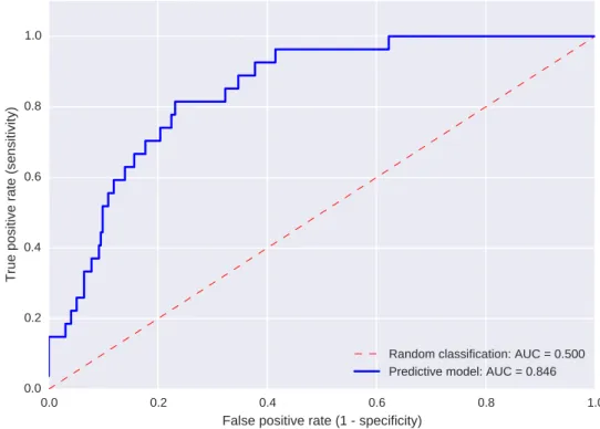
In a clinical context, the performance of a model is often evaluated via the analysis of the Receiver Operating Characteristics (ROC) curve. A ROC curve is a plot that illustrates the performance of the model based on the true and the false positive rate [28], an example of ROC curve is provided in Figure 2.4. The true positive rate is equivalent to the sensitivity and represents the ratio of positive instances that are correctly classified (e.g. percentage of sick people that have been accurately recognised as a case). The false positive rate indicates the proportion of negative samples that are incorrectly labelled as cases (e.g. percentage of healthy people diagnosed with a disease). A ROC curve can be generated only when the classifier can compute a “score” (real value) for each instance. This score, typically in the range between 0 and 1, is often intended to indicate the probability that an instance has to belong to the a specific class. The ROC curve is plotted by varying the threshold setting at which the instances are assigned to a specific class. For example, if the threshold is set to 0.2, all the samples that received a score (predicted output), equal or higher than 0.2 are predicted as positive. Once all the test samples have been classified, the sensitivity and specificity values are calculated and added as data points in the space of the true and false positive rate. ROC curves are typically used to determine the threshold that best suits the goal of the research question (e.g. at which value the sensitivity is maximised while having at least a false positive rate of 0.7). The ROC curve can also be summarised into a single value by calculating the area under it, called Area Under the ROC Curve (AUC). The AUC represents the probability that the classifier will rank a positive instance, randomly picked, higher than a randomly selected negative one (when assuming that positive samples rank higher than negatives). For a binary classification problem, a perfect classifier generates an AUC of 1, while a random
classifier (that assigns with 50% chance one of the two class labels) obtains an AUC of 0.5. Every model providing an AUC lower than 0.5 is considered to perform worse than a random one. Similar to the ROC curve, the Precision-Recall (PR) curve shows the performance of a classifier based on precision and recall. The AUPRC (area under the PR curve) summarises, as the AUC, the performance with a single value that ranges between 0 and 1. The PR curve represents a valid alternative to the ROC curve, that, on the other hand, is widely used and adopted in the biomedical field.
Fig 2.4: Example of a ROC curve summarising the performance of a predictive model.
Data are usually heterogeneous, therefore when dividing, often randomly, the instances into training and test set, one of the two sets might not properly represent the concept of the data. A standard approach used to reduce the bias of the data being split into training and test set is the cross-validation. A typical n-fold cross-validation scheme randomly divides the dataset D in n equally-sized disjoint subsets D1, D2, ..., Dn . In
turn, each fold is used as test set while the remaining n 1 are used as training set. A stratified cross-validation aims to partition the dataset into folds where the original dis-tribution of the classes is preserved [29]. The drawback of the stratified cross-validation is that it does not take into account the presence of clusters (similar samples) within each class. As observed in [30], this might lead to a distorted measure of the
perfor-mance. When dealing with datasets having a small number of observations, as typical in a biomedical context, such distortion in performances can be amplified. To solve this problem, Zeng and Martinez proposed the Distributed Balanced-Stratified Cross Validation (DB-SCV) scheme [31]. The DB-SCV is designed to assign close-by samples to di↵erent folds so that each fold will end up with enough representatives of every possible cluster. When n is equal to the total number of samples, the cross-validation is known as Leave One Out Cross Validation (LOOCV). Each instance is in turn used as test set while all the remaining are used for the training phase. Two reasons make the leave-one-out attractive, first it maximises the number of samples used for the training phase and therefore increases the chance to have and accurate model. Secondly, it does not involve random sampling (bias) as the procedure is deterministic (only one way to divide the dataset with a LOOCV) and there is no need in repeating it multiple times. On the other hand, it has been demonstrated that such approach tends to overestimate the performance of the models [30], mainly because no strat-ification can be applied. Nevertheless, when dealing with small datasets having few samples, perhaps concentrated in one class, the leave-one-out is one of the few avail-able options. Regardless the type of cross-validation chosen, the overall performance of the model are assessed by averaging the performance values obtained in each test set. Overall, with the cross-validation, it is possible to simulate the model usage and better estimate how the learning algorithm was able to generalise the concept repre-sented by the input data. In addition, this process provides a hint on how the model will perform when dealing with future instances.
2.2.2.2 The knowledge representation in supervised learning
The learning can also be classified according to the knowledge representation used to reproduce the output [32]. Russell and Norvig [33] stated that:
“
The object of the knowledge representation is to express knowledge in computer-tractable form, such that it can be used to help agents perform well.The main di↵erent knowledge representations that can be found in the supervised learning are:
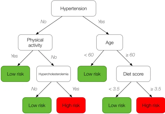
• Decision Trees are tree-like graphs that define a series of questions about the attributes to predict the label of the data samples. An example of a decision tree, for the classification of stroke risk (low or high), can be seen in Figure 2.5. Each node of the tree divides the instances according to a test over an attribute; the leaves correspond to the final predicted label. When decision trees are used to predict numeric values they are called regression trees. C4.5 is in absolute the most representative algorithm based on decision trees [34].
Hypertension
Age
Low risk
Physical activity
Low risk High risk Diet score Low risk No Yes ≥ 60 < 60 ≥ 3.5 < 3.5 No Yes
Low risk High risk
Hypercholesterolemia
Yes No
Fig 2.5: Example of a decision tree for a stroke risk classification problem.
• Classification rules consist of a series of rules that assign each instance to a class if a condition is met. The rule is usually represented using anIf-Then form: “IF condition C Then Class A”. The condition C is called rule antecedent or precondition and is defined by one or more attribute tests logically combined. The then part is called rule consequent and consists of the class prediction. A learning system that employs rules typically produces a set of di↵erent classifi-cation rules, each one matching a di↵erent area of the input space. An example
of a classification rule set is represented in Figure 2.6. RIPPER [35] and PART [36] are two of the most well known rule-based algorithms.
IF
age
≤
30
AND
student
= “no”
⟶
buy computer = “no”
IF
age
≤
30
AND
student
= “yes”
⟶
buy computer = “yes”
IF
age
> 40
AND
credit rating
= “excellent”
⟶
buy computer = “yes”
IF
age
≤
30
AND
credit rating
= “fair”
⟶
buy computer = “no”
Fig 2.6: Example of a classification rule set for a computer purchase problem.
The Learning Classifier System (LCS) is a machine learning paradigm introduced by Holland [37] that exploits evolutionary computation to develop a set of con-ditional rules (classifiers). LCSs have been extensively used in the biomedical domain as a powerful tool for knowledge discovery given their elevated inter-pretability [38]. There exist two main distinct types of LCSs: Michigan-Style and Pittsburgh-Style. In the Pittsburgh approach each individual is a complete solu-tion for the classificasolu-tion problem, tradisolu-tionally an individual is a variable-length set of rules. Conversely, in the Michigan approach, each individual is a single rule and the whole population cooperates to solve the classification problem. Al-though di↵erent, both approaches share the goal of finding sets of classifiers that provide a solution for the analysed task.
BioHEL (Bioinformatics-Oriented Hierarchical Learning) [39] is a rule-based evolutionary machine learning system designed to handle large-scale biological datasets. BioHEL generates sets of classification rules using an approach di↵ er-ent than the Michigan and Pittsburgh style: the iterative rule learning (IRL) principle. The IRL creates the classification rules sequentially using a standard genetic algorithm (GA). After every rule is generated (the best individual of the GA population), the samples from the training set covering that rule are removed. This learning process is repeated until there are no more examples in the training set. BioHEL uses an explicit default rule in each rule set, the IRL process also terminates if the system cannot generate rules that are better than the default one. The fitness function used by BioHEL is based on the Minimum Description Length (MDL) principle and is defined to promote accurate, general
and compact (simple) rules. BioHEL employs a rule representation called At-tribute List Knowledge Representation (ALKR), illustrated in Figure 2.7. ALKR has been designed to cope with biomedical data that often are large-scale, noisy, ambiguous and usually described by a large number of attributes [39]. Each classifier condition is defined by five structures: (1) the number of represented attributes (2) a list of the identifiers of the represented attributes, (3) a list of values for the represented attributes, (4) a list of the positions where each attribute can be found in the classifier and (5) the class of the classifier. The rationale behind this design is that most of the successful rules obtained from biomedical datasets contain only a few key attributes (from the large set of available ones). Hence, automatically discovering these key attributes and only keeping track of them, contributes to a substantial speed-up of the learning phase as it avoids useless match operations with irrelevant attributes. ALKR, rather than coding all the domain attributes, uses a list containing only the expressed ones, this avoids irrelevant match operations (computationally expensive) with non-expressed attributes. In addition, the ALKR structure facilitates important operations during the learning process such as specialisation and generalisation that add and remove attributes from the list with a certain probability. Overall, the ALKR provides competent learning performance and manages to reduce the system run-time considerably.
0 2 4 0.5 0.7 1 1 0 0.3 0.4 3 0 2 5 3 numAtt whichAtt predicates offsetPred class
Fig 2.7: Representation of a classifier using ALKR.
• SVMnamely Support Vector Machine, belongs to the family of the linear mod-els, a set of model-based learning approaches that expresses the output as a linear combination of the input attributes. The SVM is based on the concept of deci-sion planes that define decideci-sion boundaries [40]. A decision plane, or hyperplane,
tries to separate a set of objects that belong to di↵erent classes. Thus, the SVM attempts to generate hyperplanes that separate the samples while maximising the margin, that is the distance between data points from distinct classes. An SVM example is represented in Figure 2.8 (a). More formally, having {(xi, yi)}
withi= 1, ...l xi 2 <dand yi,2{ 1,1}, wherexi are data points andyi are the
corresponding labels, an hyperplane that separates the objects can be defined as:
f(x) = (w>·x) +b
wherewis ad-dimensional coefficient vector that is normal to the hyperplane and
b is the o↵set from the origin. A linear SVM tries to maximise the margin (the distance of the points from the hyperplane) by solving the following optimisation task: min w kwk2 2 subject to: yi(w>·x) +b 1 i= 1, .., l
This approach works well only when dealing with data that are linearly separable. If the data are non-linear, SVM, but also other linear classifiers, provides an easy and efficient way to overcome the problem. This is known as the “the kernel trick” [41] and it consists of defining a mathematical function : Kn ! H
that maps the data into a higher dimensional space where is possible to generate an hyperplane that separates objects from di↵erent classes. The most common kernel functions, for two data points x1 and x2 are:
I RBF (Radial basis function): exp kx1 x2k2 I Polynomial: (x1·x2+ 1)d
I Sigmoid: tanh (x1·x2)
where d and are user-defined parameters (common default values are 3 and 1/(number of features), respectively).
• ANN namely Artificial Neural Network [42], is inspired by the natural neurons and is another example of a linear model. A perceptron represents an artificial neuron, an ANN simply consists of a set of perceptrons connected to each other. The output of the ANN is generated as the weighted sum (strength) of the connections between perceptrons. The set of perceptrons that connects the input nodes (input layer) with the output nodes is defined as thehidden layer. A typical ANN with one hidden layer is illustrated in Figure 2.8. The back propagation algorithm is commonly used to train the ANN and identify the best set of weights for a particular problem [43]. When having multiple levels of representation, such as an ANN with many hidden layers, we fall into the class of techniques called deep learning, nowadays one of the most studied field of machine learning. Deep learning methods are defined by multiple levels of representation (i.e. layers) that are generated by composing simple (non-linear) modules (i.e. neurons). Each module transforms the representation at one level (starting with the input) into a representation at a higher, slightly more abstract level [44]. With such composition of layers, very complex functions can be learned, thus very complex problems can be addressed. Di↵erent types of deep neural networks exist, each one better suited for a specific task. For example, convolutional networks (neural networks where the connectivity pattern between the neurons is inspired by the organisation of the animal visual cortex) are ideal for the analysis of data with structured variables such as images, text and audio, recurrent networks (neural networks that contain connection within neurons of the same layer) perform well in the analysis of sequential data such as text and speech, autoencoders are special types of neural networks that receive unlabelled data (unsupervised learning) and aim to transform the input into the output with the least possible amount of distortion (typically used for dimensionality reduction), etc. Deep learning is currently the fastest growing field in machine learning, new successful approaches are continuously proposed to tackle a wide range of problems from predicting the potential of drug molecules to the analysis of particle accelerator data. An interesting overview of deep learning can be found in [44], more detailed information are outside the scope of this thesis.
Hyperplane
Support vector Support vector
Margin
(a) Support Vector Machine
Input #1
Input #2
Input #3
Input layer Hidden layer Output layer
Output
Weight wi,j
(b) Artificial Neural network
Fig 2.8: Example of linear models: an SVM classifier (left) and a simple artificial neural network (right).
• Bayesian networks are acyclic directed graphs in which each node represents a random variable and the edges define probabilistic dependencies among the corresponding random variables. Bayesian networks can be used as models to represent the probability that a certain sample belongs to one class:
P(lung cancer =yes|smoking=no, positiveXray =yes) =?
The probability of the event to occur can be calculated by applying the Bayes’ theorem:
P (A|B) = P (B |A)P (A)
P(B)
where are P (A) and P (B) are the probabilities of observing A and B without regard to each other, P(A|B) and P(B |A) are the probabilities of observing the eventA given that the eventB is true and viceversa. Naive Bayes [45] is the most simplistic Bayesian network classifier. It has been shown to perform well on many classification problems despite its simplicity and strong assumptions [46]. More complex classifiers have been presented based the Bayesian approach. For example, ABC-Miner learns the structure of a Bayesian network Augmented Naive-Bayes (a Bayesian network graph with no restrictions on the number of parents of a node) using Ant Colony Optimisation [47]. Its extension has also been used for the hierarchical classification of ageing-related proteins [48].
![Fig 1.1: Example of the possible applications of machine learning in biomedicine as illustrated in [10].](https://thumb-us.123doks.com/thumbv2/123dok_us/9777283.2469462/23.892.287.740.369.753/fig-example-possible-applications-machine-learning-biomedicine-illustrated.webp)
![Fig 2.1: The central dogma of molecular biology and the connections with the type of -omics data obtained from each tier (based on diagram by Lmaps [21]).](https://thumb-us.123doks.com/thumbv2/123dok_us/9777283.2469462/32.892.215.793.122.519/central-dogma-molecular-biology-connections-obtained-diagram-lmaps.webp)
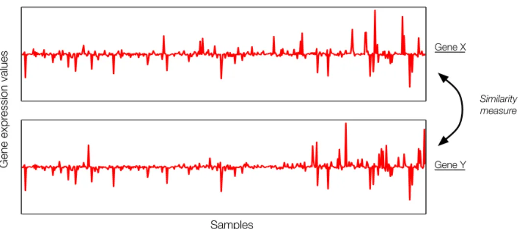
![Fig 2.12: Comparison of the similarity measures calculated with PCC and MIC for di↵erent type of associations between two variables [88].](https://thumb-us.123doks.com/thumbv2/123dok_us/9777283.2469462/56.892.263.766.437.667/fig-comparison-similarity-measures-calculated-erent-associations-variables.webp)