The de-biased group Lasso estimation for varying coefficient models

Title The de-biased group Lasso estimation for varying coefficient models

Author(s) Honda, Toshio Citation

Issue Date 2019-08

Type Technical Report

Text Version publisher

URL http://hdl.handle.net/10086/30520

Graduate School of Economics, Hitotsubashi University

Discussion Paper Series No. 2018-04

The de-biased group Lasso estimation

for varying coefficient models

Toshio HONDA

First version : November 2018

This version : August 2019

The de-biased group Lasso estimation

for varying coe

ffi

cient models

Toshio Honda

There has been a lot of attention on the de-biased or de-sparsified Lasso since it was proposed in 2014. The Lasso is very useful in variable selection and obtaining initial es-timators for other methods in high-dimensional settings. However, it is well-known that the Lasso produces biased estimators. Therefore several authors simultaneously proposed the de-biased Lasso to fix this drawback and carry out statistical inferences based on the de-biased Lasso estimators. The de-biased Lasso procedures need desirable estimators of high-dimensional precision matrices for bias correction. Thus the research is almost limited to linear regression models with some restrictive assumptions, generalized linear models with stringent assumptions and the like. To our knowledge, there are a few papers on linear regression models with group structure, but no result on structured nonpara-metric regression models such as varying coefficient models. In this paper, we apply the de-biased group Lasso to varying coefficient models and closely examine the theoretical properties and the effects of approximation errors involved in nonparametric regression. Some simulation results are also presented.

Keywords: high-dimensional data; B-spline; varying coefficient models; group Lasso; bias correction.

1

Introduction

We consider the following high-dimensional varying coefficient model : Yi =

p

j=1

gj(Zi)Xi,j+i, (1)

where (Yi,Xi,Zi), i = 1, . . . ,n, are i.i.d. observations, Yi is a dependent variable, Xi =

(Xi,1, . . . ,Xi,p)T ∈RpandZi∈ Rare random covariates, and an unobserved errorifollows the

normal distribution with mean zero and varianceσ2

independently of (Xi,Zi). Note thata T _is

the transpose of a vector or matrixa. In (1),Zi is a key variable sometimes called an index

variable andXi,1satisfiesXi,1≡1. Besides,Zitakes values on [0,1] andgj(Zi)j=1, . . . ,p,are

Toshio Honda is Professor, Graduate School of Economics, Hitotsubashi University, 2-1 Naka, Kunitachi, Tokyo 186-8601, Japan (Email: [email protected]). This research is supported by JSPS KAKENHI Grant Number JP 16K05268.

unknown smooth functions on [0,1] to be specified later in Section 3. The varying coefficient model is one of the most popular structured nonparametric regression models. For example, see [11] for an excellent review on varying coefficient models. Such structured nonparametric regression models alleviate the curse of dimensionality, but they allow much more flexibility in modelling and data analysis than linear regression models.

Nowadays a lot of high-dimensional datasets are available because of rapid advances in data collecting technology and it is inevitable to apply structured nonparametric regression models to such kinds of high-dimensional datasets for more flexible data analysis. In this pa-per, we takep=O(ncp_{) for some positive constantc}

pand this excludes ultra-high dimensional

cases. This is because the technical conditions and the proofs are complicated and we give priority to readability. In practice we have to pay some cost for nonparametric estimation of coefficient functions and have some difficulty dealing with ultra-high dimensional cases. Note that the actual dimension ispL, whereLis the dimension of the spline basis.

In high-dimensional settings, even if pis very large compared to the sample size n, the number of active or relevant covariates are much smaller than p and we need some vari-able selection procedures for high-dimensional datasets like the Lasso(e.g.[26] and [1]), the SCAD(e.g.[7]), feature screening procedures based on marginal models or some index be-tween the dependent variable and individual covariates(e.g.[9]), and forward variable selec-tion procedures(e.g.[30] and [17]). [21] is an excellent review paper of feature screening procedures. The adaptive Lasso and the group Lasso are important variants of the Lasso. For example, see [35], [33], [22]. There are too many papers on high-dimensional issues to mention and we just name a few books for recent developments, [3], [13], and [27].

Several authors considered ultra-high dimensional or high-dimensional varying coefficient models by employing the group Lasso(e.g.[31]), the group SCAD(e.g.[5]), feature screening procedures based on marginal models and so on (e.g.[8] and [20]), and forward variable selec-tion procedures(e.g.[6]). In [14] and [15], the authors considered Cox regression models with high-dimensional varying coefficient structures.

The Lasso is very useful in variable selection and obtaining initial estimators for other methods like the SCAD in high-dimensional settings. However, it is well-known that the Lasso is not necessarily selection consistent and produces biased estimators. We need some suitable initial estimators or screening procedures to reduce the number of covariates when we implement the SCAD. Screening procedures are based on marginal models or some index betweenYi and individual covariates. And the procedures crucially depend on assumptions

like the one that marginal models reflect the true model faithfully. When we need some reli-able estimates maintaining the original high dimensionality, these procedures may not be very useful. The SCAD has the nice oracle property, but it gives no information about removed or

unselected covariates. When a covariate of interest is not selected, we have no information other than being not selected. On the other hand, the de-biased Lasso gives some useful in-formation such as p-values. The SCAD selects covariates and set the coefficient to be 0 if the covariate is not selected. Statistical inference under the original model is impossible for the SCAD.

Several authors([34], [18], and [28]) simultaneously proposed the de-biased Lasso to fix the fore-mentioned drawbacks of the Lasso and the SCAD. It is also called the de-sparsified Lasso. We can carry out statistical inferences based on the de-biased Lasso estimators while maintaining the high dimensionality and get information about all the covariates of the orig-inal high-dimensional model. The de-biased Lasso procedures need desirable estimators of high-dimensional precision matrices for bias correction. Thus the research is almost limited to linear regression models with some restrictive assumptions, generalized linear models with stringent assumptions, and the like. To our knowledge, there are a few papers on linear re-gression models with group structure(e.g. [23], [25]). The authors of these papers derived interesting and useful results. But we have found no result on structured nonparametric re-gression models such as varying coefficient models. Besides their assumptions on covariate variables cannot cover our setup since we have to deal withW defined in (4) and our design matrixW has a special structure due to the B-spline basis and{Zi}.

We have to examine the properties carefully by carrying out conditional arguments on{Zi}

and using the properties of the B-spline basis. We also have to take care of approximation er-rors to true coefficient functions. Our purpose is to estimate coefficient functions and different from that of [23] and [25] does not deal with random design cases. Both of them consider only linear models. In this paper, we apply the de-biased group Lasso to varying coefficient models and closely examine the theoretical properties of estimated coefficients and the effects of approximation errors involved in nonparametric regression.

This paper is organized as follows. In Section 2, we describe the de-biased group Lasso procedure for varying coefficient models. Then we present our assumptions and main theo-retical results in Section 3. Simulation study results are presented in Section 4. The results suggest that the proposed de-biased group Lasso will work well. Additional numerical results are given in the Supplement. We prove the main theoretical results in Section 5. The technical proofs are also relegated to the supplement.

We end this section with some notation used throughout the paper.

In this paper, we write A Bwhen we defineAby B. C,C1,C2,. . ., are generic positive

constants and their values may change from line to line. Note thatan∼bnmeansC1<an/bn<

C2and thata∨banda∧bstand for the maximum and the minimum ofaandb, respectively.

complement and the number of the elements of an index set S ⊂ {1, . . . ,p}, respectively. When we have two random vectorsU and V, U|V stands for the conditional distribution of U on V. And N(μ, σ2) means the normal distribution with mean μand variance σ2 and we writeU ∼ N(μ, σ2_{) when U follows the normal distribution with mean μ and variance σ}2_.

Convergence in distribution is denoted by→d.

For a vectora, a is the Euclidean norm and g 2and g ∞stand for theL2and sup norms

of a function g on the unit interval, respectively. We denote the maximum and minimum eigenvalues of a symmetric matrix A by λmax(A) and λmin(A), respectively. For a matrix A, A Fandρ(A) stand for the Frobenius and spectral norms, respectively. We write (A)s,t for the

(s,t) element of a matrixAandIk is thek-dimensional identity matrix.

2

The de-biased group Lasso estimator

In this section, we define the de-biased group Lasso estimatorbfrom the group Lasso estima-torβ. Then we need some desirable estimator of the precision matrix ofΣin Assumption S1 below and we denote the estimator byΘ. We presentΘafter we defineβandb.

•Regression spline model : First we explain our regression spline model for (1). We de-note theL-dimensional equispaced B-spline basis on [0,1] byB(z)= (B1(z), . . . ,BL(z))T with

L

k=1Bk(z)≡ √

L, not 1. We employ a quadratic or smoother basis here. The conditions onL and coefficient functions are given Section 3, e.g. in Assumptions G and L.

By choosing a suitableβ0j ∈RL, we can approximategj(z) byBT(z)β0j as

gj(z)= BT(z)β0j+rz j(z),

whererz j(z) is a small approximation error. Then (1) is rewritten as

Yi= p

j=1

Xi,jBT(Zi)β0j+ri+i, (2)

whereri =p_j=1(g(Zi)−BT(Zi)β0j)Xi,j. Note that we takeβ0j =0∈RLifgj(z)≡0.

Now we define new pL-dimensional covariate vectors and then×(pL) design matrix for the regression spline model as

W_i X_i⊗B(Zi)=(Xi,1BT(Zi), . . . ,Xi,pBT(Zi))T ∈RpL, (3)

where⊗is the Kronecker product, and W ⎛ ⎜⎜⎜⎜⎜ ⎜⎜⎜⎜⎜ ⎜⎜⎜⎝ WT 1 ... WT_n ⎞ ⎟⎟⎟⎟⎟ ⎟⎟⎟⎟⎟ ⎟⎟⎟⎠=(W1, . . . ,Wp), (4)

whereW is ann×(pL) matrix andWjis ann×Lmatrix. Note that we haveni.i.d. W_i ∈RpL. We write Wj =(W(1)_j , . . . ,W_j(L)) and W(_jl)= ⎛ ⎜⎜⎜⎜⎜ ⎜⎜⎜⎜⎜ ⎜⎜⎜⎝ W₁(l_,)_j ... W_n(l_,)_j ⎞ ⎟⎟⎟⎟⎟ ⎟⎟⎟⎟⎟ ⎟⎟⎟⎠∈Rnforl=1, . . . ,L.

Note thatWjis a covariate matrix forgj(Zi)Xi,jand thatW_i(_,l_j)= Xi,jBl(Zi) is an element ofW.

By using the above notation, we can representnobservations in a matrix form :

Y = p j=1 Wjβ0j+r+ =W β0+r+, where Yi =WT_iβ0+ri+i, (5) Y=(Y1, . . . ,Yn)T,r=(r1, . . . ,rn)T,=(1, . . . , n)T, andβ0 =(βT₀₁, . . . , βT_0p)T ∈RpL.

We state a standard assumption on the design matrixW. This is assumed throughout this paper.

Assumption S1

ΣE(W_iWT_i) and λmin(Σ)>C1

for some positive constantC1. Note thatΣis a (pL)×(pL) matrix.

Note that Σ = n−1E(WT_{W) and we usually denote the inverse of Σ by Θ, not Σ}−1_{, as}

in the literature on high-dimensional precision matrices. The sample version of Σ isΣ n−1WTW. When pL is larger than n, we cannot define the inverse of Σ. Therefore we need a reliable substitute of the inverse ofΣ in high-dimensional setups and we denote our estimator of the inverseΘbyΘ. We define ann×(p−1)LmatrixW−jby removingWj from

W =(W1, . . . ,Wp). We consider regression ofWj toW−jwhen we construct ourΘ. •Group Lasso estimatorβ: We define the group Lasso estimatorβfor (2) and (5) :

β =(βT₁, . . . ,βT_p)T argmin β∈RpL 1 n Y−W β 2_+2λ 0P1(β) , (6)

whereβ = (βT₁, . . . , βT_p)T with βj ∈ RL for j = 1, . . . ,p, λ0 is a suitably chosen tuning

pa-rameter, and P1(β)

p

j=1 βj . We also use this P1(·) for vectors of smaller dimension.

We describe the properties of this group Lasso estimator in Proposition 1 for completeness although the proposition is almost known.

The first order condition of the optimality ofβyields

−1

nW

T_(Y−Wβ)+λ

0κ0=0∈RpL, (7)

whereκ0 = (κT_0,1, . . . , κT_0,p)T withκ0,j ∈ RL for j = 1, . . . ,p, κ0,j ≤ 1 for j = 1, . . . ,p, and

•De-biased group Lasso estimatorb : Thisβis a biased estimator due to the L1 penalty

as we mentioned in Section 1. Thus by constructingΘ such thatΘΣis sufficiently close to IpL, we define our de-biased group Lasso estimatorb =(bT₁, . . . ,bTp)T ∈ RpL withbj ∈ RL for

j=1, . . . ,pfor the varying coefficient model (1) and (5) as _{bβ+Θλ0κ0=β+} 1 nΘW T_{(Y−Wβ) (8)} =β+ΘΣ(β0−β)+ 1 nΘW T_(r+) =β0+ 1 n(ΘΣ−IpL)(β0−β)+ 1 nΘW T_(r+) =β0+ 1 nΘW T_−Δ 1+ Δ2,

where we used (7) in the first line,

Δ1=(ΔT1,1, . . . ,Δ T 1,p) T 1 n(ΘΣ−IpL)(β−β0)∈R pL_, Δ2=(ΔT2,1, . . . ,Δ T 2,p)T 1 nΘW T_r∈RpL_, Δ1 = ⎛ ⎜⎜⎜⎜⎜ ⎜⎜⎜⎜⎜ ⎜⎜⎜⎝ Δ1,1 ... Δ1,p ⎞ ⎟⎟⎟⎟⎟ ⎟⎟⎟⎟⎟ ⎟⎟⎟⎠ 1n(ΘΣ−IpL)(β−β0)∈ R pL_{, Δ} 2 = ⎛ ⎜⎜⎜⎜⎜ ⎜⎜⎜⎜⎜ ⎜⎜⎜⎝ Δ2,1 ... Δ2,p ⎞ ⎟⎟⎟⎟⎟ ⎟⎟⎟⎟⎟ ⎟⎟⎟⎠ 1nΘW T_r∈RpL_,

andΔ1,j ∈ RL and Δ2,j ∈ RL for j = 1, . . . ,p. We will prove that Δ1 and Δ2 are negligible

compared ton−1ΘWT _{in Propositions 3 and 4, respectively and closely examinen}−1_ΘWT

in Proposition 5 in Section 3.

The evaluation ofΔ2requires more smoothness of the coefficient functionsgj(z) than usual

as in Assumption G in Section 3. This is because it is difficult to evaluate the effects of approx-imation errors while maintaining high-dimensionality as shown in the proof of Proposition 3. Any model may have some kind of approximation error and it is very important to exam-ine such effects in the de-biased Lasso method closely. If we are interested in only some of Xi,1, . . . ,Xi,p, not all of them, we do not have to compute the wholeband should concentrate

on only the corresponding blocks.

•Construction of Θ : At the end of this section, we construct Θ by employing the group Lasso and adapting the idea in [28] to the current group structure. Note that our construction is different from those of [23] and [25] and that we can exploit just the standard R package for the Lasso for computation. We also describe some idea of how toΘin (9)-(11) after the notation.

We need some more notation before we present ourΘ. Hereafter, we writea⊗2 aaT _for

Σ−j,j, and a (p−1)L×(p−1)LmatrixΣ−j,−j: Σj,k E{X1,jX1,kB⊗2(Z1)}= 1 nE(W T jWk) Σj,−j E[{X1,j(X1,1, . . . ,X1,j−1,X1,j+1, . . . ,X1,p)} ⊗B⊗2(Z1)]= 1 nE(W T jW−j) Σ−j,−j E[{(X1,1, . . . ,X1,j−1,X1,j+1, . . . ,X1,p)T}⊗2⊗B⊗2(Z1)]= 1 nE(W T −jW−j)

andΣ₋j,j ΣT_j,−j. Note that they can be defined also fromΣas its submatrices. Furthermore we

define a (p−1)L×LmatrixΓjasΓj Σ−1₋j,−jΣ−j,j and writeΓj=(γ(1)j , . . . ,γ

(L)

j ), whereγ

(l)

j ∈

R(p−1)L _{forl = 1, . . . ,L. We need to estimate this Γ}

j to defineΘ. In this paper, we estimate

Γj = Σ−1_−j,−jΣ−j,j = (γ_l(1), . . . , γ(_lL)) columnwise by employing the group Lasso differently from

[25]. See Remark 1 at the end of this section.

To present an idea on the construction ofΘ, we give some insightful expressions such as (10)-(12). Then we define ann×LmatrixEjand its columnsη(jl)∈ Rn, j=1, . . . ,L,as

Ej =(η(1)_j , . . . , η(_jL))Wj−W−jΓj. (9) SinceΣ₋j,j−Σ−j,−jΓj =n−1E(W₋T_jEj)=0, we have 1 nE(W T_E 1)= 1 nE{W T_(W 1−W−1Γ1)}=(Θ−11,1,0,0, . . . ,0) T · · · · 1 nE(W T_E j)= 1 nE{W T_(W j−W−jΓj)}=(0,Θ−1j,j,0, . . . ,0)T (10) · · · · 1 nE(W T_E p)= 1 nE{W T (Wp−W−pΓp)}=(0, . . . ,0,0,Θ−p,1p) T_,

where symmetricL×LmatricesΘj,jwill be defined shortly. The above equations imply

1 nE{W T_(E 1, . . . ,Ep)} ⎛ ⎜⎜⎜⎜⎜ ⎜⎜⎜⎜⎜ ⎜⎜⎜⎜⎜ ⎜⎜⎜⎜⎜ ⎜⎜⎜⎜⎜ ⎜⎜⎝ Θ−1 1,1 0 0 · · · 0 0 Θ−1_2,2 0 · · · 0 0 0 Θ−1_3,3 · · · 0 ... ... ... ... ... 0 0 0 · · · Θ−1_p,p ⎞ ⎟⎟⎟⎟⎟ ⎟⎟⎟⎟⎟ ⎟⎟⎟⎟⎟ ⎟⎟⎟⎟⎟ ⎟⎟⎟⎟⎟ ⎟⎟⎠ −1 =IpL. (11)

Recalling thatn−1E(WTW)= Σand (9), we defineΘby employing the sample version of the LHS of (11). Thus we need to estimateΓj, j=1, . . . ,p. See also (19) below.

LetΘj,kbe anL×Lsubmatrix ofΘexactly asΣj,kis a submatrix ofΣ. Then we have

Θ−1 j,j = Σj,j−Σj,−jΣ−₋1j,−jΣ−j,j = 1 nE(E T jEj)= 1 nE(W T jEj). (12)

We explain how we estimate Γj. Looking at (9) andn−1E(W₋T_jEj) = 0 columnwise, we have η(l) j =W (l) j −W−jγ (l) j ∈R n_{, l=} 1, . . . ,Land j=1, . . . ,p,

and then we estimateΓj =(γ(1)_l , . . . , γ_l(L)) columnwise by employing the group Lasso:

γ(l) j =(γ (l)T j,1 , . . . ,γ (l)T j,j−1,γ (l)T j,j+1, . . . ,γ (l)T j,p ) T _argmin γ∈R(p−1)L 1 n W (l) j −W−jγ 2_+2λ(l) j P1(γ) , (13) where P1(γ) is defined as in (6),γ( l) j,k ∈ R L _{for k j, γ = (γ}T 1, . . . , γ T j−1, γ T j+1, . . . , γ T p)T with

γk ∈ RL fork j, andλ(jl) is a suitably chosen tuning parameter. We deal with the theoretical

properties ofγ(_jl)in Proposition 2 in Section 3. As in (7), we have −1 nW T −j(W (l) j −W−jγ (l) j )+λ (l) j κ (l) j =0∈ R (p−1)L_{, (14)}

whereκ(_jl) =(κ(_jl_,1)T, . . . , κ(_j,l)_jT₋₁, κ(_jl_,)_jT₊₁, . . . , κ(_jl_,)_pT)T withκ(_jl_,)_k ∈RLfork j, κ(_jl_,)_k ≤1 fork j, and

κ(l) j,k =γ (l) j,k/γ (l) j,k if γ (l) j,k 0.

Collectingγ(_jl), κ(_jl_,)_k, and regression residuals into matrices, respectively, we define (p− 1)L×LmatricesΓj andKjand ann×LmatrixEjas

_Γj (γ(1)_j , . . . ,γ(_jL)), Kj (κ(1)_j , . . . ,κ(_jL)), and EjWj−W−jΓj (15) and write _Γj =(ΓTj,1, . . . ,Γ T j,j−1,ΓTj,j+1, . . . ,Γ T j,p)T, Kj =(KTj,1, . . . ,K T j,j−1,KTj,j+1, . . . ,K T j,p)T, and Ej =W(−ΓTj,1, . . . ,−Γ T j,j−1,IL,−ΓTj,j+1, . . . ,−Γ T j,p) T_, (16)

whereΓj,k(k j) and Kj,k(k j) areL×Lmatrices. Then by (14), we have

1 nW

T

−jEj =KjΛj, (17)

whereΛj =diag(λ(1)_j , . . . , λ(_jL)). The elements of the RHS of (17) will be small because of the

properties of the group Lasso. Recall thatn−1E(W₋T_jEj)=0.

We are ready to defineΘby adapting the idea of [28] to the current setup. LetT2

j be our

estimator ofΘ−1_j,j and defined later. See also (9), (11), and (16).

ΘT ⎛ ⎜⎜⎜⎜⎜ ⎜⎜⎜⎜⎜ ⎜⎜⎜⎜⎜ ⎜⎜⎜⎜⎜ ⎜⎜⎜⎜⎜ ⎜⎜⎝ IL −Γ2,1 −Γ3,1 · · · −Γp,1 −Γ1,2 IL −Γ3,2 · · · −Γp,2 −Γ1,3 −Γ2,3 IL · · · −Γp,3 ... ... ... ... ... −Γ1,p −Γ2,p −Γ3,p · · · IL ⎞ ⎟⎟⎟⎟⎟ ⎟⎟⎟⎟⎟ ⎟⎟⎟⎟⎟ ⎟⎟⎟⎟⎟ ⎟⎟⎟⎟⎟ ⎟⎟⎠ ⎛ ⎜⎜⎜⎜⎜ ⎜⎜⎜⎜⎜ ⎜⎜⎜⎜⎜ ⎜⎜⎜⎜⎜ ⎜⎜⎜⎜⎜ ⎜⎜⎝ T2 1 0 0 · · · 0 0 T2 2 0 · · · 0 0 0 T2 3 · · · 0 ... ... ... ... ... 0 0 0 · · · T2 p ⎞ ⎟⎟⎟⎟⎟ ⎟⎟⎟⎟⎟ ⎟⎟⎟⎟⎟ ⎟⎟⎟⎟⎟ ⎟⎟⎟⎟⎟ ⎟⎟⎠ −1 . (18)

Hereafter the second matrix on the RHS will be denoted by diag(T₁−2, . . . ,T_p−2). Note thatT−2_j stands for the inverse ofT2

j and is an estimator ofΘj,j.

(16)-(18) give the following equations if we takeT2

j 1 nW T j Ej. Compare (11) and (19), too. _ΣΘT ₌ 1 nW T (WΘT)= 1 nW T (E1, . . . ,Ep)diag(T1−2, . . . ,T−2p ) (19) = ⎛ ⎜⎜⎜⎜⎜ ⎜⎜⎜⎜⎜ ⎜⎜⎜⎜⎜ ⎜⎜⎜⎜⎜ ⎜⎜⎜⎜⎜ ⎜⎜⎝ T2 1 K2,1Λ2 K3,1Λ3 · · · Kp,1Λp K1,2Λ1 T₂2 K3,2Λ3 · · · Kp,2Λp K1,3Λ1 K2,3Λ2 T₃2 · · · Kp,3Λp ... ... ... ... ... K1,pΛ1 K2,pΛ2 K3,pΛ3 · · · T2p ⎞ ⎟⎟⎟⎟⎟ ⎟⎟⎟⎟⎟ ⎟⎟⎟⎟⎟ ⎟⎟⎟⎟⎟ ⎟⎟⎟⎟⎟ ⎟⎟⎠ diag(T₁−2, . . . ,T−2p ) and _ΣΘT _−I pL= ⎛ ⎜⎜⎜⎜⎜ ⎜⎜⎜⎜⎜ ⎜⎜⎜⎜⎜ ⎜⎜⎜⎜⎜ ⎜⎜⎜⎜⎜ ⎜⎜⎝ 0 K2,1Λ2T₂−2 K3,1Λ3T₃−2 · · · Kp,1ΛpTp−2 K1,2Λ1T₁−2 0 K3,2Λ3T₃−2 · · · Kp,2ΛpTp−2 K1,3Λ1T1−2 K2,3Λ2T2−2 0 · · · Kp,3ΛpTp−2 ... ... ... ... ... K1,pΛ1T₁−2 K2,pΛ2T₂−2 K3,pΛ3T₃−2 · · · 0 ⎞ ⎟⎟⎟⎟⎟ ⎟⎟⎟⎟⎟ ⎟⎟⎟⎟⎟ ⎟⎟⎟⎟⎟ ⎟⎟⎟⎟⎟ ⎟⎟⎠ . (20)

The elements of the off-diagonal blocks will be small due to the properties of the group Lasso in (13).

Taking the transpose of (20), we obtain

ΘΣ−IpL= ⎛ ⎜⎜⎜⎜⎜ ⎜⎜⎜⎜⎜ ⎜⎜⎜⎜⎜ ⎜⎜⎜⎜⎜ ⎜⎜⎜⎜⎜ ⎜⎜⎝ 0 T−2T 1 Λ1K T 1,2 T−2 T 1 Λ1K T 1,3 · · · T−2 T 1 Λ1K T 1,p T−2T 2 Λ2K T 2,1 0 T− 2T 2 Λ2K T 2,3 · · · T− 2T 2 Λ2K T 2,p T−2T 3 Λ3K T 3,1 T−2 T 3 Λ3K T 3,2 0 · · · T−2 T 3 Λ3K T 3,p ... ... ... ... ... T−2T p ΛpKT_p,1 Tp−2TΛpK_pT_,2 T−2p TΛpKT_p,3 · · · 0 ⎞ ⎟⎟⎟⎟⎟ ⎟⎟⎟⎟⎟ ⎟⎟⎟⎟⎟ ⎟⎟⎟⎟⎟ ⎟⎟⎟⎟⎟ ⎟⎟⎠ . (21) We denote (T−2_j )T _byT−2T

j . We will closely examine

T−_j2TΛjKTj,k =T− 2T j ⎛ ⎜⎜⎜⎜⎜ ⎜⎜⎜⎜⎜ ⎜⎜⎜⎝ λ(1) j κ (1)T j,k ... λ(L) j κ (L)T j,k ⎞ ⎟⎟⎟⎟⎟ ⎟⎟⎟⎟⎟ ⎟⎟⎟⎠ to deal withΔ1in Proposition 3.

Finally note that T2

j = n− 1_WT j Ej, our estimator of Θ− 1 j,j = Σj,j −Σj,−jΣ− 1 −j,−jΣ−j,j, satisfies

min_1≤j≤pρ(T2j) >C with probability tending to 1 for some constantCas proved in Lemma 6

in Section 5. See also (12) about this definition ofT2

In Section 4, we choseλ0andλ(

l)

j by cross validation. In the next section, we give

theoret-ically proper ranges of these tuning parameters. But we have no theory for tuning parameter selection.

Remark 1 In [25], the authors considered fixed design regression models and estimated all the columns ofΓj simultaneously in a single Lasso-type penalized regression. On the other

hand, we estimateΓj columnwise and we can apply the standard theory and also employ the

standard R package to get our estimator of Γj. We can define another estimator of Θ just

formally even if we estimate Γj simultaneously. Then the properties will be different from

those of this paper and we cannot apply the standard Lasso theory and R packages then.

3

Theoretical results

In this section, we state the standard result on the group Lasso estimatorsβandγ(_jl)in Propo-sitions 1 and 2 together with technical assumptions. Then we evaluateΔ1 and Δ2 in (8) and

ΘΣΘT _{in Propositions 3-5. Finally we state the main result on the de-biased group Lasso}

esti-matorbin Theorem 1. We will prove Propositions 3-5 in Section 5. Theorem 1 immediately follows from those propositions. Propositions 1 and 2 will be proved in the Supplement since we can prove them by just following the standard arguments in the Lasso literature. The proofs of all the technical lemmas will also be given in the Supplement.

•Basic assumptions : We describe some notation and assumptions before we present the results on the group Lasso estimators. We define the set of active covariates and the number of active covariates :

S0 {j| gj 2 >0} ⊂ {1, . . . ,p} and s0|S0|. (22)

We begin with some definitions to state basic assumptions on the properties of covariates of our varying coefficient model:

X_i=(Xi,2, . . . ,Xi,p)T and X˘_i =X_i−μX(Zi),

whereμX(Zi)= (μX,2(Zi), . . . , μX,p(Zi))T is the conditional mean ofXi givenZi. We denote the

conditional covariance matrix ofX_i givenZi by ΣX(Zi). We define X_i by removing the first

constant element fromX_idefined in (1). Assumption VC

(1)E(Xi,j) = 0, j = 2, . . . ,p. Besides, μX,j ∞ < C1for j = 2, . . . ,pandC2 < λmin(ΣX(z))≤

λmax(ΣX(z))< C3 uniformly inzon [0,1] for some positive constantsC1,C2, andC3. Recall

(2)There is a constant σ2 _{independent ofZ}

i such that E{exp(αTX˘_i)|Zi} ≤ exp( α 2σ2/2) for

anyα∈Rp−1_.

(3) The index variable Zi has density fZ(z) satisfying C4 < fZ(z) < C5 on [0,1] for some

positive constantsC4andC5.

The second one, the sub-Gaussian design assumption, allows us to use Bernstein’s inequal-ity. The first two assumptions may look restrictive. However, we need to construct a desirable estimator of a precision matrix and even more restrictive assumptions such as normality are imposed in [28] and [19]. Especially, the arguments in [19] crucially depend on the normality assumption on the design matrix although it has improved the previous results on the de-biased Lasso. The assumption on{i}is the standard one in the literature of the de-biased Lasso. In

[4], the authors developed the theory of the de-biased Lasso for linear models without nor-mality or sub-Gaussian assumption on design matrices, but they need a restrictive assumption on the order of psuch as p nand other alternative conditions. The third one is a standard assumption for varying coefficient models.

Next we state the assumptions on coefficient functions. Assumption G

(1)gj(z), j=1, . . . ,p, are three times continuously differentiable.

(2)If we choose suitableβ0j ∈ RL anddj j =1, . . . ,p, the approximation errorri,j defined as

ri,j =gj(Zi)−BT(Zi)β0jsatisfies |ri,j|<C1L−3djfori=1, . . . ,nand j∈ S0, j∈S0 dj <C2, and j∈S0 d2_j <C3 (23)

for some positive constantsC1,C2, andC3.

In this paper,_kL₌₁Bk(z) ≡ √

L. Then we have for some positive constantsC1 andC2that C1 < λmin(ΩB) ≤ λmax(ΩB) <C2, whereΩB =

1 0 B(z)B

T_{(z)dz. See e.g. [16] about this fact.}

We employ a quadratic or smoother basis. We give a remark on other spline bases in Remark 2 later in this section.

The former half of Assumption G may be a little more restrictive. However, we need this assumption to evaluateΔ2. If we takedj = gj ∞+ gj ∞+ gj ∞+ g

(3)

j ∞and some suitable

β0j, this{dj}satisfies the first one in (23). See e.g. Corollary 6.26 of [24]. This{dj}should

satisfy the second and third ones in (23). Note that we takeβ0j =0 for j S0 and thatg(3)_j (z)

is the third order derivative ofgj(z).

We denote the conditional mean and variance of L3

j∈S0ri,jXi,j given Zi by μr(Zi) and

σ2

r(Zi), respectively. Then under Assumptions VC and G, we have

for some positive constantsC1andC2. The above results, the sub-Gaussian design assumption,

and the use of Bernstein’s inequality imply

|ri| <C3(logn)1/2L−3 (24)

uniformly iniwith probability tending to 1 for some positive constantC3. Recallriis defined

in (2).

• Results on β: The theoretical results on the Lasso crucially depends on the deviation condition (Lemma 1) and the restrictive eigenvalue (RE) condition or a similar one (Lemma 2). If both of the conditions are established, the standard theoretical results (Proposition 1) follow almost automatically from them.

Lemma 1 Suppose that Assumptions VC and G hold and that(L−3logn+ n−1Llogn)→0. Then for some large constant C, we have

P_∞(n−1WT)<C

Llogn

n and P∞(n

−1_WT_r)<CL−3_logn

with probability tending to 1, whereP_∞(v)max_1≤j≤p vj forv =(vT₁, . . . ,vTp)T ∈ RpLwith

vj ∈RLfor j=1, . . . ,p.

We also use P_∞(·) for vectors of lower dimension as we use P1(·).

Some preparations are necessary to define the RE condition. For an index setS ⊂ {1, . . . ,p} and a positive constantm, we define a subset ofRpL_{as in the literature on the Lasso :}

Ψ(S,m){β ∈RpL|P1(β_S)≤mP1(βS) andβ 0},

whereβ_Sconsists of{βj}j∈S, βS consists of{βj}_j∈S, and P1(·) is conformably adjusted to the

dimension of the arguments. Recallβj ∈ RL in this paper. Then we define φ2_Ω(S,m) for a

non-negative (pL)×(pL) matrixΩas

φ2

Ω(S,m)_β∈min_Ψ(S,m)β

T_Ωβ

βS 2.

In the theory of the Lasso, φ2

Σ(S0,m) plays a crucial role and the lower bound is given in

Lemma 2 below.

Lemma 2 Suppose that Assumptions VC and S1 hold and that s0

n−1_L3_logn→_{0. Then}

2φ2_Σ(S0,3)≥φ2_Σ(S0,3)≥λmin(Σ) with probability tending to 1.

Notice that the second inequality is trivial from the definition ofφ2

Σ(S0,3) and always holds.

The next result may be almost known, but we present and prove it for completeness.

Proposition 1 Suppose that Assumptions VC, S1, and G hold and that (s0

n−1L3_logn)∨

(L−3logn+ n−1Llogn)→0. Then ifλ0 =C(L−3logn+

n−1Llogn)for sufficiently large C, we have with probability tending to 1,

1 n W(β−β0) 2_≤18 λ 2 0s0 φ2 Σ(S0,3) and P1(β−β0)≤24 λ0 s0 φ2 Σ(S0,3) .

We will prove this proposition in the Supplement including the case where we have some prior knowledge onS0. Note thatC in the definition of λ0 is from Lemma 1. We will follow the

proof in [4] and we can also deal with the weighted group Lasso as in [4] with just conformable changes. Note that [4] considered the adaptive Lasso for linear regression models. We didn’t present the adaptively weighted Lasso version since the notation is very complicated in the current setup of the group Lasso procedures. If an estimator has the oracle property, e.g. the SCAD estimator and a kind of suitably weighted Lasso estimators as in [10], it is not biased and we don’t have to apply the de-biased procedure to those estimators. However, as we mentioned before, no statistical inference is possible while maintaining the original high-dimensionality.

•Results onγ(_jl) for Θ: We consider the properties of another group Lasso estimator γ(_jl) defined in (13). We deal with the deviation condition and the RE condition in Lemma 3 and Lemma 4, respectively. Then Proposition 2 about the group Lasso estimatorγ(_jl) in (13) follows almost automatically from them.

We define the active index setS(_jl) ⊂ {1, . . . , j−1, j+1, . . . ,p}ofγ(_jl)in almost the same way asS0 ofβ0and let s(_jl) |S(_jl)|. We assumeS(_jl)is not empty since we can include some

index in it even if it is actually empty. We need some technical assumptions. Assumption S2

(1) γ(_jl) ≤C1uniformly inl(1≤l≤L) and j(1≤ j≤ p) for some positive constantC1.

(2)λmax(Σj,j)≤C2uniformly in j(1≤ j≤ p) for some positive constantC2.

Assumptions S1 and S2(2) imply

C3≤λmin(Θ−1j,j)= 1 λmax(Θj,j) ≤λ max(Θ−1j,j)= 1 λmin(Θj,j) ≤ C4 (25)

uniformly in jfor some positive constantsC3andC4.

We give some comments on the implications of Assumptions VC, S1, and S2 to consider the properties of the group Lasso estimator ofγ(_jl)in (13). Then we writeη(_jl) =(η₁(l_,)_j, . . . , η(_nl_,)_j)T ∈

Rn_{. SinceΣ}

−j,j−Σ−j,−jΓj =0 and our observations are i.i.d., we have

E(W_i,−jη_i(_,l)_j)=0∈R(p−1)L, i=1, . . . ,n, l=1, . . . ,L, and j=1, . . . ,p, (26) where defineW_i,−j by removingXi,jB(Zi) fromW_i and we haveW−j=(W_1,−j, . . . ,W_n,−j)T.

We denote the conditional mean and variance of η(_i,l)_j given Zi by μ_η,(l)j(Zi) and σ_η,(l)2j(Zi),

respectively. Under Assumption S2(2), we have

E{η(_il_,)2_j }=E[{μ(_η,l)_j(Zi)}2+σ_η,(l)2_j(Zi)]=O(1) (27)

uniformly inl(1 ≤ l ≤ L) and j(1≤ j ≤ p). Besides, Assumptions VC and S2(1), and the properties of the B-spline basis suggest

σ(l)2

η,j ∞=O(L) (28)

uniformly in l and j. Assumption S1 is closely related to Assumption S2(1) since Γj =

Σ−1 −j,−jΣ−j,j.

We need an assumption onμ(_η,l)_j(z) similar to (28) to deal with the deviation condition. We give a comment on this assumption in Remark 3 at the end of this section.

Assumption EUnder Assumption VC, we have uniformly inl(1≤l≤ L) and j(1≤ j≤ p) ,

μ(l)

η,j ∞=O( √

L).

Next we state Assumptions on the dimension of the B-spline basisL,s0, ands(_jl). We allow

them to depend onnas long as they satisfy the assumptions. Assumption L

(1)n−1_s(l)2

j L

3_{logn→0 uniformly inl(1≤l≤ L) and j(1≤ j≤ p).}

(2)n−1s(_jl)L4_{logn→0 uniformly inl(1≤l≤L) and j(1≤ j≤ p).}

(3)n−1s2 0L

4_(logn)2 _→0.

Lemma 3 Suppose that Assumptions VC, S2, and E hold and that n−1L2_{logn→0. Then for} some large constant C, we have

P_∞(n−1W₋Tjη (l) j )<C L2_logn n

uniformly in l(1≤l≤L)and j(1≤ j≤ p)with probability tending to 1.

The convergence rate is worse than that in Lemma 1. This is due to the structure ofW, (28), and Assumption E. There may be possibility of improvement in this convergence rate. See Remark 4 at the end of this section.

Lemma 4 DefineΣ₋j,−jasΣ−j,−j 1_nW₋T_jW−j. Then suppose that Assumptions VC, S1, and L(1) hold. Then 2φ2_Σ −j,−j(S (l) j ,3)≥φ 2 Σ−j,−j(S (l) j ,3)≥λmin(Σ)

uniformly in l(1≤l≤L)and j(1≤ j≤ p)with probability tending to 1.

Proposition 2 Suppose that Assumptions VC, S1, S2, E, and L(1) hold and takeλ(_jl) =Cn−1L2_logn for sufficiently large C. Then we have

1 n W−j(γ (l) j −γ (l) j ) 2 _≤18λ (l)2 j s (l) j λmin(Σ) and P1(γ(jl)−γ (l) j )≤24 λ(l) j s (l) j λmin(Σ) uniformly in l(1≤l≤L)and j(1≤ j≤ p)with probability tending to 1.

ActuallyCin Proposition 2 can depend onland jif it belongs to some suitable interval. Note thatCin the definition ofλ(_jl)is from Lemma 3.

•Results onb : We present Propositions 3-5. Hereafter we assume the conditions on the tuning parametersλ0andλ(_jl)in Propositions 1 and 2.

Proposition 3 Suppose that Assumptions VC, G , S1, S2, E, and L(1)-(3) hold. Then we have

Δ1,j <C

1 n1/2 ·

s0L2logn n1/2

uniformly in j(1≤ j≤ p)with probability tending to 1 for sufficiently large C.

Proposition 4 Suppose that Assumptions VC, G , S1, S2, E, and L(1)(2) hold. Then we have

Δ2,j <C·L−3

L

l=1

s(_jl)1/2logn≤CL−5/2logn(max

l,j s

(l)

j )

1/2

uniformly in j(1≤ j≤ p)with probability tending to 1 for sufficiently large C.

We give a comment on possibility of some improvements on Proposition 4 in Remark 5 at the end of this section. It is just a conjecture that we have not proved yet.

We introduce some more notation before Proposition 5. We denote the residual vectors from the group Lasso in (13) byη(_jl) Wj−W₋T_jγ(_jl) ∈ Rn and note thatEj =(η(1)_j , . . . ,η(_jL)),

whereEjis ann×Lmatrix. Besides, we set

ΩΘΣΘT ₌ 1 nΘW T_WΘT (29) ={diag(T₁−2, . . . ,Tp−2)}T 1 n(E1, . . . ,Ep) T_(E 1, . . . ,Ep)diag(T1−2, . . . ,Tp−2)

and define its submatrixΩj,k in the same way as Σj,k and Θj,k are defined as submatrices of

Σand Θ, respectively. We used (16) and (18) in the last line. Note thatΩ is a (pL)×(pL) matrix and it is the conditional variance matrix ofn−1/2_ΘWT_{. Recall diag(T}−2

1 , . . . ,Tp−2) is

Proposition 5 Suppose that Assumptions VC, G , S1, S2, E, and L(1)(2) hold and fix a positive integer m. For any{j1, . . . , jm} ⊂ {1, . . . ,p}, we define a symmetric matrixΔas

Δ ⎛ ⎜⎜⎜⎜⎜ ⎜⎜⎜⎜⎜ ⎜⎜⎜⎝ Ωj1,j1 · · · Ωj1,jm ... ... ... Ωjm,j1 · · · Ωjm,jm ⎞ ⎟⎟⎟⎟⎟ ⎟⎟⎟⎟⎟ ⎟⎟⎟⎠− ⎛ ⎜⎜⎜⎜⎜ ⎜⎜⎜⎜⎜ ⎜⎜⎜⎝ Θj1,j1 · · · Θj1,jm ... ... ... Θjm,j1 · · · Θjm,jm ⎞ ⎟⎟⎟⎟⎟ ⎟⎟⎟⎟⎟ ⎟⎟⎟⎠. Then we have |λmin(Δ)| ∨ |λmax(Δ)| →0 uniformly in{j1, . . . , jm}with probability tending to 1.

Our main result, Theorem 1, immediately follows from Propositions 3-5. Recall thatΔ1=

(ΔT

1,1, . . . ,Δ

T

1,p)T andΔ2 = (Δ₂T_,1, . . . ,ΔT_2,p)T. We give a comment on spline bases in Remark 2

below.

Theorem 1 Suppose that Assumptions VC, G , S1, S2, E, and L(1)-(3) hold. Then the de-biased estimator is represented as

_{b−β0 =} 1

nΘW−Δ1+ Δ2 and we have

Δ1,j =op(n−1/2) and Δ2,j <Clogn·L−5/2(max l,j s

(l)

j )

1/2

uniformly in j(1 ≤ j ≤ p)with probability tending to 1 for sufficiently large C. Besides, we have n−1/2_ΘWT_{| {X}

i,Zi}ni=1 ∼ N(0, σ 2

Ω) andΩconverges in probability to Θblockwise as

defined in Proposition 5.

Remark 2 This remark concerns other spline bases. We can take another spline basis B(z) satisfyingB(z) = AB(z) andC1 < λmin(AAT) ≤ λmax(AAT) <C2 for some positive constants C1andC2. For example, an orthonormal basisB(z) satisfying

B(z)(B(z))T_{dz= I}

L. This is

because we deal with and evaluate everything blockwise. We use the desirable properties of the B-spline basis in the proofs and then we should apply the conformable linear transformation blockwise.

We consider applications of Theorem 1. Recall we have maxj∈S0 gj−B T_β

0j ∞ =O(L−3)

by Assumption G.

•Statistical inference under the original high-dimensional model

(1) gj 2 : Suppose we use a spline basis satisfying the orthonormal property in Remark

is the estimator. Recall again that the SCAD gives no information of gj 2 when this j is

not selected. Most of screening procedures rely on an assumption like the one that marginal models faithfully reflect the true model. It is important to have a de-biased estimator of gj 2

for any jbased on the initial and original high-dimensional varying coefficient model (1). Theorem 1 suggests that for any fixed j,

bj−β0j =Op

L

n

if √n−1L/{logn· L−5/2_(max

l,js(jl))1/2} → ∞. This reduces to L6/{n(logn)2maxl,js(jl)} → ∞.

Note that β0j − gj 2 = O(L−3) uniformly in junder Assumption G and this approximation

error is negligible compared to (L/n)1/2_.

In addition to point estimation of gj 2, we can carry out hypothesis testing ofH0 : gj 2=

0 vs.H1 : gj 20 for any j. Then we can approximate the distribution of bj by bootstrap

for j S0to compute the critical value as we did in the simulation studies.

(2) gj(z) : We estimategj(z) withBT(z)bj. SinceBT(z)β0j−gj(z)=O(L−3) under Assumption

G, this approximation error is negligible compared to the effect ofΔ2and (L/n)1/2. Note that

{n−1_BT_(z)Ω

j,jB(z)}1/2∼(L/n)1/2in probability. Therefore for any fixed j, we have

n1/2BT(z)(bj−β0j)/{BT(z)Ωj,jB(z)}1/2 d

→N(0, σ2) (30) if √n−1_L/{_logn· _L−2_(max

l,js(_jl))1/2} → ∞. This reduces to L5/{n(logn)2maxl,js(_jl)} → ∞.

This condition may be a little restrictive. However, a smallerL may work practically from Remarks 4 and 5 below. See Subsection S.2.3 in the Supplement for some numerical examples of confidence bands forgj(z).

We state some remarks here. Those remarks are about possible improvements of our as-sumptions and we have not proved them yet.

Remark 3 This remark is about Assumption E. First we consider the case ofl = 1 for sim-plicity of notation. Forl=1,μ(1)_η,j(Zi) andσ(1)2_η,j (Zi),i=1, . . . ,n, are written as

μ(1)

η,j(Zi)=a(1)j T{μX(Zi)⊗B(Zi)} and σ(1)2_η,j (Zi)=a(1)j T[ΣX(Zi)⊗ {B(Zi)}⊗2]a(1)j ,

wherea(1)_j (1,0, . . . ,0,−γ(1)_j T)T _{∈ R}pL_{and a}(1)

j = O(1) uniformly in jfrom Assumption

S2. (28) easily follows from the local support property ofB(z). This holds for the otherl. On the other hand,μ(_η,l)_j(Zi) is rewritten for generallas

μ(l) η,j(Zi)=μX,j(Zi)Bl(Zi)− s∈S(_jl) μX,s(Zi)b(_sl_,)_jTB(Zi) and s∈S(_jl) b(_sl_,)_j 2 = γ(_jl) 2,

whereb(_sl_,)_j is part ofγ_j(l). If_s∈S(l)

j b (l)

s,j <Cors

(l)

j <Cuniformly inland jfor some positive

constantC, Assumption E holds because of the local support property of the B-spline basis. Besides since only a finite number of elements ofB(z) are not zero for any zdue to its local support property, Assumption E seems to be a reasonable one.

Remark 4 This remark refers to possible improvement on Lemma 3. In Lemma 3, we should evaluate the expression inside the expectation on the LHS of (31).

E L m=1 1 n n i=1 Xi,kBm(Zi)η(il,)j 2 = 1 nE (X1,kη(₁l_,)_j)2 L m=1 B2m(Z1) ≤C1 L nE{(X1,kη (l) 1,j) 2_{} (31)} ≤ C1L n E{|X1,k| 2p1}1/p1_E{|η(l) 1,j| 2p2}1/p2

for some positive constantC1 and (p1,p2) satisfying 1/p1 +1/p2 = 1. Note that we used

Assumption VC and the fact for some positive constantC3,Lm=1B2m(Z1)<C3Luniformly in Z1here. If we take p1 =4 andp2 =4/3, we have (31)=O(L3/2/n) and this suggests there may

be possibility of improvement in convergence rate up to n−1L3/2_{logn. We have not proved}

this conjecture yet.

Remark 5 This remark is about possible improvement on Proposition 4. Note that ⎛ ⎜⎜⎜⎜⎜ ⎜⎜⎜⎜⎜ ⎜⎜⎜⎝ Δ2,1 ... Δ2,p ⎞ ⎟⎟⎟⎟⎟ ⎟⎟⎟⎟⎟ ⎟⎟⎟⎠ T = 1 nr T_W ⎛ ⎜⎜⎜⎜⎜ ⎜⎜⎜⎜⎜ ⎜⎜⎜⎜⎜ ⎜⎜⎜⎜⎜ ⎝ IL −Γ2,1 · · · −Γp,1 −Γ1,2 IL · · · −Γp,2 ... ... ... ... −Γ1,p −Γ2,p · · · IL ⎞ ⎟⎟⎟⎟⎟ ⎟⎟⎟⎟⎟ ⎟⎟⎟⎟⎟ ⎟⎟⎟⎟⎟ ⎠ diag(T₁−2, . . . ,T−2p ) = 1 nr T_(E 1, . . . ,Ep)diag(T1−2, . . . ,T−2p ) and 1 nr T_η(l) j = 1 nr T_η(l) j + 1 nr T_W −j(γ(jl)−γ (l) j ).

Recall the definition ofEj in (15) andEj =(η(1)j , . . . ,η

(L) j ). Since |n−1rTW−j(γ_j(l)−γ(_jl))| ≤(n−1 r 2)1/2(n−1 W−j(γ(_jl)−γ(_jl)) 2)1/2 ≤CL−3(logn)1/2(max l,j s (l) j ) 1/2 L2_logn n

uniformly in jwith probability tending to 1 for some positive constantC, this is small enough. Hence we have only to evaluate n−1rT_η(l)

j . Recalling ri = j∈S0Xi,j(gj(Zi)− B T_(Z i)β0j) and η(l) j = W (l) j −W−jγ (l) j , we conjecture thatn−1r T_η(l)

j is much smaller than Op(L−3) given in the

4

Numerical studies

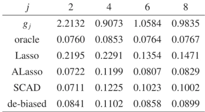
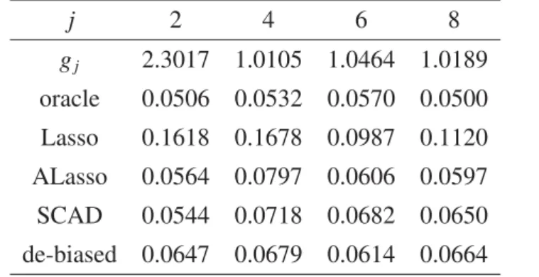
In this section, we present the results of simulation studies. The proposed de-biased group Lasso estimator may look complicated. However, it worked well in the simulation studies and the results imply that this de-biased group Lasso estimator is quite promising.

In the studies, we present the results on hypothesis testing of whether gj 2 =0 or not for j=1, . . . ,12 in Models 1-3 defined below. We also present some more simulation results and a real data application in Section S.2 in the Supplement.

We used the cv.gglasso function of the R package ‘gglasso’ version 1.4 on R x64 3.5.0. The package is provided by Profs Yi Yang and Hui Zou. See [32] for more details. We chose tuning parameters by using the CV procedure of the cv.gglasso function. First we computed

β by using the CV procedure and then corrected the bias of it to getb. We also used the CV procedure when we computedΘ. We didn’t optimizeb with respect to λ0 because it

took too much of time even for one repetition. We used an orthonormal spline basis which is constructed from the quadratic equispaced B-spline basis.

In the three models, Zi follows the uniform distribution on [0,1] Xi,1 ≡ 1, and {Xi,j}p_j=2

follows a stationary Gaussian AR(1) process withρ=0.5. We took E{Xi,2}=0 and E{X2_i,2}=1

and Zi and {Xi,j} p

j=2 are mutually independent. As for the error term, we took i ∼ N(0,3).

We tried two cases, (L,p,n,Repetition number) = (5,250,250,200) and (5,350,350,200). Note that the actual dimension is pL = 1250 and 1750. Besides, the tuning parameters were determined by the data and one iteration needs 61 runs of the group Lasso with very many covariates. Therefore it took a long time for only one case of each model.

In Model 1, we set

g2(z)=2+2 sin(πz), g4(z)=2(2z−1)2−2, g6(z)=1.8 log(z+1.718282), g8(z)=2.5(1−z).

All the other functions are set to be 0 and irrelevant. In Model 2, we set g2(z)=2+2(2z−1)3, g4(z)=2 cos(πz), g6(z)= 1.8 1+z2, g8(z)= exp(1+z) 3.4 . All the other functions are set to be 0 and irrelevant.

In Model 3, we set g2(z)=2+2 sin(πz), g4(z)=2(2z−1)2−2, g6(z)= 1.8 1+z2, g8(z)= exp(1+z) 3.4 , g10(z)=1.8 log(z+1.718282), g12(z)=2 cos(πz). All the other functions are set to be 0 and irrelevant.

We considered hypothesis testing of

H0 : gj 2=0 vs. H1 : gj 2>0 (32)

for j=1, . . . ,12 in Models 1-3. We computed the critical values from the result that √n(bj−

β0j) is approximately distributed as N(0,Ωj,j) in Theorem 1. Then bj 2 is the estimator of

gj 2since we used an orthonormal B-spline basis here. We compared bj 2and the simulated

critical value. The nominal significance levels are 0.05 and 0.10.

In Tables 1-12, each entry is the rate of rejectingH0. Tables 1, 3, 5, 7, 9, and 11 are for

relevant j(H1is true) and Tables 2, 4, 6, 8, 10, and 12 are for irrelevant j(H0is true).

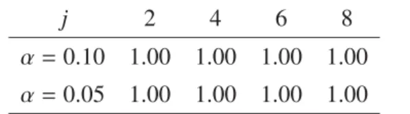
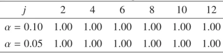
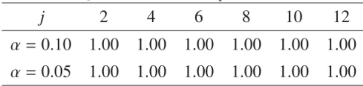
As shown in Tables for relevant covariates (H1), the rejection rate is 1.00 for any case.

As for irrelevant covariates (H0), the actual significance levels are close to the nominal ones

except for j = 7 in Models 1 and 2 and j = 7,9 in Model 3. Note that the standard errors are 0.022(α = 0.10) and 0.016(α = 0.05) since the repetition number is 200 due to the long computational time. We also tried 6 more cases where everygj(z) is replaced withgj(z)/

√

2. There is no significant differences and the results of the 6 cases are presented in the supple-ment. These simulation results imply that our de-biased Lasso procedure is very promising for statistical inference under the original high-dimensional model, i.e. statistical inference without variable selection.

Table 1: H1for Model 1 withp=250 andn=250

j 2 4 6 8

α=0.10 1.00 1.00 1.00 1.00

α=0.05 1.00 1.00 1.00 1.00

Table 2: H0for Model 1 withp=250 andn=250

j 1 3 5 7 9 10 11 12

α =0.10 0.10 0.06 0.06 0.18 0.12 0.08 0.15 0.08

α =0.05 0.06 0.02 0.02 0.13 0.06 0.04 0.08 0.06

Table 3: H1for Model 2 withp=250 andn=250

j 2 4 6 8

α=0.10 1.00 1.00 1.00 1.00

Table 4: H0for Model 2 withp=250 andn=250

j 1 3 5 7 9 10 11 12

α =0.10 0.11 0.11 0.18 0.18 0.12 0.08 0.14 0.12

α =0.05 0.06 0.06 0.10 0.11 0.06 0.04 0.08 0.05

Table 5: H1for Model 3 withp=250 andn=250 j 2 4 6 8 10 12

α =0.10 1.00 1.00 1.00 1.00 1.00 1.00

α =0.05 1.00 1.00 1.00 1.00 1.00 1.00

Table 6: H0for Model 3 withp=250 andn=250

j 1 3 5 7 9 11

α =0.10 0.12 0.07 0.05 0.22 0.22 0.15

α =0.05 0.07 0.04 0.03 0.14 0.16 0.10

Table 7: H1for Model 1 withp=350 andn=350

j 2 4 6 8

α=0.10 1.00 1.00 1.00 1.00

α=0.05 1.00 1.00 1.00 1.00

Table 8: H0for Model 1 withp=350 andn=350

j 1 3 5 7 9 10 11 12

α =0.10 0.10 0.03 0.05 0.16 0.11 0.07 0.10 0.08

α =0.05 0.06 0.02 0.02 0.12 0.06 0.05 0.06 0.05

Table 9: H1for Model 2 withp=350 andn=350

j 2 4 6 8

α=0.10 1.00 1.00 1.00 1.00

Table 10: H0for Model 2 with p=350 andn=350

j 1 3 5 7 9 10 11 12

α =0.10 0.09 0.10 0.10 0.16 0.11 0.06 0.11 0.08

α =0.05 0.04 0.04 0.06 0.10 0.06 0.04 0.06 0.05

Table 11: H1for Model 3 with p=350 andn=350 j 2 4 6 8 10 12

α =0.10 1.00 1.00 1.00 1.00 1.00 1.00

α =0.05 1.00 1.00 1.00 1.00 1.00 1.00

Table 12: H0for Model 3 with p=350 andn=350

j 1 3 5 7 9 11

α =0.10 0.09 0.05 0.07 0.22 0.20 0.10

α =0.05 0.07 0.03 0.02 0.17 0.14 0.07

5

Proofs of theoretical results

In this section, we prove Propositions 3-5. We state two technical lemmas before we prove the propositions. These lemmas will be verified in the Supplement.

We defineL×LmatricesBj,kandBj,kfor j=1, . . . ,pandk=1, . . . ,pas

Bj,k 1 n E T jEk and Bj,k 1 nE(E T jEk)

See (15) and (9) for the definitions ofEjandEj. Note that and

Bj,j = Σj,j−Σj,−jΣ−1₋j,−jΣ−j,j= Θ−1j,j and Bj,k =E ⎧⎪⎪ ⎪⎪⎪⎪⎨ ⎪⎪⎪⎪⎪ ⎪⎩ ⎛ ⎜⎜⎜⎜⎜ ⎜⎜⎜⎜⎜ ⎜⎜⎜⎝ η(1) 1,j ... η(L) 1,j ⎞ ⎟⎟⎟⎟⎟ ⎟⎟⎟⎟⎟ ⎟⎟⎟⎠(η(1)1,k, . . . , η (L) 1,k) ⎫⎪⎪ ⎪⎪⎪⎪⎬ ⎪⎪⎪⎪⎪ ⎪⎭. (33)

We establish the convergence ofBj,k toBj,kin Lemma 5.

Lemma 5 Suppose that Assumptions VC, S1, S2, E, and L(1)(2) hold. Then Bj,k−Bj,k F →0

In the next lemma, we establish the desirable properties of T2

j. Recall that ρ(A) is the

spectral norm of a matrixA.

Lemma 6 Suppose that Assumptions VC, S1, S2, E, and L(1)(2) hold. Then we have (a) and (b).

(a) For some positive constants C1 and C2, we have C1 < ρ(T2j) = ρ(T2jT) < C2and 1/C2 <

ρ(T−2

j )=ρ(T−

2T

j )<1/C1uniformly in j(1≤ j≤ p)with probability tending to 1.

(b) T2

j − Θ−1j,j F → 0 and sup x=1 (Tj−2 − Θj,j)x → 0 uniformly in j(1 ≤ j ≤ p) with

probability tending to 1.

Now we begin to prove Propositions 3-5

Proof of Proposition 3)Since (21) and the properties ofκ(_jl_,)_kbelow (14) imply

Δ1,j =T−2j TΛj kj KT_j,k(βk−β0k) and |λ(l) j kj κ(l)T j,k (βk−β0k)| ≤max_a,b λ (b) a P1(β−β0), we have uniformly in j, Δ1,j ≤max a,b λ (b) a ρ(T− 2 j )L 1/2 P1(β−β0). (34)

Recall that maxa,bλ(ab) =O(

n−1_L2_{logn) in Proposition 2. By (34), Lemma 6, and the bound}

of P1(β−β0) from Proposition 1, we have

Δ1,j ≤Cλ0s0

L3_logn

n (35)

uniformly in jwith probability tending to 1 for some positive constantC.

The desired result follows from (35) and the condition onλ0 in Proposition 1. Hence the

proof of the proposition is complete. Proof of Proposition 4)Write

(ΔT_2,1, . . . ,ΔT_2,p)=(n−1WTr)TΘT =(n−1WTr)T ⎛ ⎜⎜⎜⎜⎜ ⎜⎜⎜⎜⎜ ⎜⎜⎜⎜⎜ ⎜⎜⎜⎜⎜ ⎜⎜⎜⎜⎜ ⎜⎜⎝ IL −Γ2,1 −Γ3,1 · · · −Γp,1 −Γ1,2 IL −Γ3,2 · · · −Γp,2 −Γ1,3 −Γ2,3 IL · · · −Γp,2 ... ... ... ... ... −Γ1,p −Γ2,p −Γ3,p · · · IL ⎞ ⎟⎟⎟⎟⎟ ⎟⎟⎟⎟⎟ ⎟⎟⎟⎟⎟ ⎟⎟⎟⎟⎟ ⎟⎟⎟⎟⎟ ⎟⎟⎠ diag(T₁−2, . . . ,T_p−2).