Can you GET Me Now? Estimating the Time-to-First-Byte
of HTTP Transactions with Passive Measurements
Emir Halepovic, Jeffrey Pang, Oliver Spatscheck
AT&T Labs - Research180 Park Avenue Florham Park, NJ, United States
{emir,jeffpang,spatsch}@research.att.com
ABSTRACT
Cellular network operators have a compelling interest to monitor HTTP transaction latency because it is an impor-tant component of the user experience. Existing techniques to monitor latency require active probing or use passive anal-ysis to estimate round-trip time (RTT). Unfortunately, it is impractical to use active probing to monitor entire cellular networks, and RTT is only one component of HTTP latency in cellular networks. This paper presents a new passive tech-nique to estimate HTTP transaction latency that overcomes the scaling and completeness limitations of prior approaches. We validate our technique in an operational cellular network and present results for traffic in the wild.
Categories and Subject Descriptors
C.2.3 [Computer-Communication Networks]: Network Operations
Keywords
Time To First Byte, Round-Trip Time, Network measure-ment, Cellular, Wireless, Mobile
1.
INTRODUCTION
Quick application response time has always been a cru-cial component of a satisfactory user experience [10], and recent studies suggest that differences of only 250 millisec-onds will cause a user to visit a Web site less often [2]. As more and more applications migrate to the Web and inter-act with the cloud, the latency of network protocol transac-tions is an increasingly important component of overall user response time. In particular, this trend implies a growing importance of HTTP transaction latency, as HTTP is the dominant protocol for the mobile Web, RESTful APIs, and video streaming [3].
Cellular network operators have a compelling interest to monitor the latency of HTTP transactions because changes in their networks can directly influence these latencies. A
Permission to make digital or hard copies of all or part of this work for personal or classroom use is granted without fee provided that copies are not made or distributed for profit or commercial advantage and that copies bear this notice and the full citation on the first page. To copy otherwise, to republish, to post on servers or to redistribute to lists, requires prior specific permission and/or a fee.
IMC’12,November 14–16, 2012, Boston, Massachusetts, USA.
Copyright 2012 ACM 978-1-4503-1705-4/12/11 ...$15.00.
standard measure of HTTP transaction latency is the total time-to-first-byte (TTFB). The total TTFB is informally de-fined as the time elapsed from a user’s request for an object to the reception of the first byte of that object. This time represents the lower bound on the delay the user will experi-ence before an application can start rendering the requested content. Of particular interest to network operators is the TTFB of a single HTTP transaction, i.e., time between the start of the TCP handshake and the arrival of the HTTP response at the user device. This elapsed time, which we refer to as TTFB hereafter for brevity, captures all the la-tency components that a cellular network can directly in-fluence.1
Unfortunately, conventional methods to measure TTFB rely on using active probing tools,2
which in practice limits the scale and representativeness of measurements to a small number of vantage points. This limitation is par-ticularly problematic for wireless network operators because it is impractical to run probes at all physical locations that their users will visit and physical context plays a large role in the wireless network latency users experience.
As a consequence, passive estimation techniques are gen-erally preferred to measure latency at scale. For exam-ple, well-known passive techniques estimate round-trip time (RTT) by measuring the arrival times of packets at the probe location [7, 8, 9, 16]. However, these prior approaches have drawbacks that limit their usefulness as a proxy for TTFB. First, prior approaches do not capture additional delays that may occur prior to the first packet being sent over the net-work. These delays are common and significant in cellular networks due to layer 2 connection setup signaling [13]. Sec-ond, approaches that only measure TCP handshake time don’t account for the transmission delay of the HTTP re-quest and response, which can be significantly larger than TCP handshake packets. Finally, the same approaches don’t account for server delay in processing the HTTP request. As a result, prior passive latency estimation techniques provide only limited visibility into changes that can impact HTTP response time in cellular networks.
In this paper, we design and evaluate a new passive mea-surement technique to estimate TTFB, taking into account the signaling and large packet transmission delays specific to cellular networks. Our approach works at a large scale and only requires information available within the network
1
The TTFB of a single HTTP transaction excludes potential delays due to DNS and HTTP redirects included in the total TTFB, but we find that a large fraction of HTTP transac-tions are not preceded by these delays (Section 3.3).
2
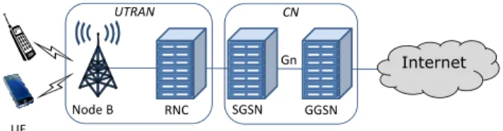
Internet Gn GGSN SGSN RNC Node B UE CN UTRAN
Figure 1: UMTS network architecture.
core, which meets two key challenges faced by a network op-erator. The main insight in our TTFB estimation approach is to utilize TCP timestamps (user domain) as well as the arrival times of packets at the probe location (network do-main). Our approach addresses the limitations of previous techniques and challenges caused by peculiarities of traffic in the wild. This allows the operator to fully quantify the influence on TTFB of RTT, cellular network latency, con-nection setup delay, transmission time of HTTP messages, and server processing delay.
Finally, we present measurement results of TTFB in a deployment on a large U.S. cellular network. We find that TTFB can better reflect user response time than RTT, as connection setup signaling, which RTT ignores, comprises up to 68% of total TTFB. Comparison of TTFB values reveals up to 72.5% difference across domains, and up to 36% across applications, whereas RTT shows no apprecia-ble difference. We believe our work demonstrates a practical method for operators to monitor a critical component of the mobile user experience.
2.
BACKGROUND AND RELATED WORK
The most significant component of TTFB is the network latency. In cellular data networks, the network latency of delivering a packet comprises of three components: radio connection setup time, radio access network (RAN) schedul-ing and transmission, and core network transmission. To illustrate, consider a UMTS network (Figure 1). When a User Equipment (UE) such as a smartphone wants to send a packet, the UMTS Terrestrial Radio Access Network (UTRAN) must first allocate a radio resource control (RRC) connection for the UE if it has not already done so. Second, the UTRAN must schedule and then deliver the packet from the UE to the Core Network (CN). Finally, the packet is sent through the core network and the Internet to the destina-tion. RAN scheduling and core network transmission typi-cally incur RTTs of 100s of milliseconds on 3G networks [15] and 50-60 milliseconds in 4G Long Term Evolution (LTE) networks [5]. A new HTTP connection will typically incur two RTTs in a TTFB, one for the TCP 3-Way Hand Shake (3WHS) and one for the HTTP request and response. While these latencies are significant, radio connection setup time often adds an order of magnitude higher delay.
Radio connection setup delay is the time it takes for the UTRAN to allocate a radio connection to the UE. To under-stand why the connection setup delay is significant, we must understand the RRC state machine [11]. To efficiently uti-lize the radio resources, both UTRAN and UE maintain the state machine, which is synchronized via signaling on the control channel. There are typically three RRC states in a UMTS network: IDLE, CELL-FACH, CELL-DCH.3
The state machine transitions to a higher resource state (state
3
The same state machine mechanism applies when
addi-promotion), i.e., IDLE to CELL-DCH, when the UE has more data to send/receive and to a lower resource state (state demotion), i.e., CELL-DCH to CELL-FACH, when the UE has less data to send/receive. The reason for a sig-nificant connection setup delay is a state promotion, which involves signaling latency between the UE and the UTRAN. This latency is variable because signaling messages can be lost due to contention. Since RRC state is demoted after only a few seconds [12], a connection setup delay will typi-cally occur for each user-initiated request.
The state promotion time is 1.5 to 2 seconds in UMTS [12], 260 milliseconds in LTE [5], and 80 ms in Wi-Fi [5]. These delays are an order of magnitude larger than the correspond-ing RAN schedulcorrespond-ing and core network transmission delays, and they grow even larger when there is contention for radio resources. In addition, operators will evolve existing cellu-lar networks by introducing new RRC states and by tuning RRC timers, which will change the magnitude and frequency of the connection setup delay [11]. Hence, to effectively mon-itor TTFB in cellular data networks, it is imperative that any estimation technique has the capability to measure all three components of network latency.
2.1
Limitations of Existing Techniques
Previous passive techniques attempt to estimate the RTT of TCP connections that pass through a passive packet mon-itor along the connections’ end-to-end path. In a UMTS cel-lular data network, the monitor is typically located on the Gn link (Figure 1), where all cellular data traffic passes, be-cause they are usually located in a small number of physical locations [4, 14].4
There are several approaches to estimate RTT. SYN-ACK estimation uses the interval between the SYN and acknowl-edgment (ACK) packets of the TCP 3WHS, and Slow-Start estimation measures intervals between bursts of data packets within a minimum of 5 consecutive data packets [8]. Jaiswal, et al. [7] estimate RTT by replicating the sender’s state ma-chine to infer congestion window size. Veal, et al. [16] es-timate RTT as inter-arrival time between data and ACK packets matched by TCP timestamps.
All these techniques estimate network latency by record-ing the arrival time of IP packets at the monitor. Thus, a crucial limitation of these approaches is that they can not capture the connection setup delay that occurs before the first IP packet of a transaction leaves the UE for the UTRAN. Moreover, they don’t measure the transmission time incurred for the HTTP request and response. In this paper, we design a new approach that overcomes this lim-itation by passively inferring the timing of packets at the UE.
3.
DESIGN
In order to capture all potential components of cellular network latency, we focus on measuring the TTFB of HTTP transactions that begin with new TCP connections.5
Fig-ure 2 depicts the typical packet exchange at the beginning tional states are used, such as URA-PCH, and in LTE and Wi-Fi with PSM [5].
4
In LTE, the equivalents to the Gn link are the S1u and S11 links.
5
These transactions are most likely to be user initiated be-cause typical web servers tear down persistent HTTP con-nections after only a few seconds [1].
r
0t
0t
1r
1t
2r
2 SYN SYN-ACK ACK HTTP-GET HTTP-DATA GET-ACK DATA-ACK SERVER UE (OS)R T T
1 PROBET T F B
Q
UE (Radio)S T T
R T T
2r
21r
22 T S 0 T S 1 T S 2t
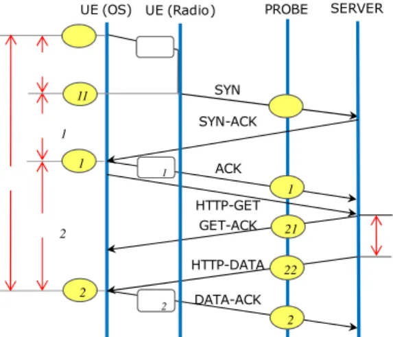
11Figure 2: Typical HTTP data transfer.
Table 1: TTFB and its components.
Metric Actual Estimate
T T F B t2−t0 G(T S2−T S0) ST T t11−t0 G(T S1−T S0)−(r1−r0) RT T1 t1−t11 (r1−r0) RT T2 t2−t1 (r2−r1) Q unknown (r22−r21) G unknown r2−r1 T S2−T S1
of such HTTP transaction. The vertical lines represent elapsed time at the UE operating system (OS), radio inter-face, probe, and server. Bubbles labeledtiandrirepresent
arrival times of packets, and T Si are TCP timestamps in
packets, which we describe in Section 3.1. The SYN, SYN-ACK, and ACK packets comprise the TCP 3WHS, while the HTTP-GET and HTTP-DATA packets correspond to the HTTP request and the first packet of the response. As RRC state transition is the largest part of the radio connec-tion setup, we refer to this delay as State Transiconnec-tion Time (ST T) hereafter. Qis the server processing delay.
We define the actual TTFB as the time elapsed between the SYN packet departure and the arrival of the first HTTP-DATA packet at the UE, i.e. t2−t0. We stress that our
definition of TTFB differs from the conventional one by not including DNS latency, as explained later. However, it in-cludes the complete TCP 3WHS, STT when it occurs, as well as the HTTP request and the first packet of the re-sponse. Previous estimation techniques only used arrival timesri to estimate latency (e.g., RTT =r1−r0 [14, 8]),
thereby missing the crucialST T that occurs betweent0and r0. Unfortunately,t0andt2are only directly measurable at
the UE and available only for active probing techniques. In this section, we describe how we can estimate t2−t0 and
break down its constituent latency components using only information measured at the probe. Our approach is sum-marized in Table 1.
3.1
Challenges
The na¨ıve approach to estimating TTFB at the probe would be as the inter-arrival time between the SYN and DATA-ACK, i.e.,r2−r0. This estimate would be correct
if the latency between the UE and the probe is always the same. However, as we already explained, the delayr0−t0
is often much larger than the delaysr1−t1 andr2−t2due
toST T. To overcome this limitation of the na¨ıve approach, we need to estimatet0 andt2directly.
To do this estimation, we leverage the observation that many TCP connections include the TCP timestamp option (75% of the top 500 servers in previous work [16] and 85% of TCP connections in our dataset). This option adds two fields to the TCP header: Timestamp Value (TSval) and Timestamp Echo Reply (TSecr) [6]. The sender sets TSval to the time at which the segment was sent, and the receiver echoes the TSval of the most recently received segment in TSecr. Therefore, eachti is represented by the
correspond-ingT Siin each TCP packet (Figure 2).
Under the assumption that the clock the sender uses to computeT S0 andT S2 has a known frequency
1
G′ ticks/sec,
we would have the simple equivalence t2−t0 =G′(T S2− T S0). Unfortunately,
1
G′ is not known and it depends on the
device generating the timestamp. Moreover, we will not be able to measure TTFBs with any finer time resolution than
G′because the timestamps are quantized to integral values.
Thus, two challenges are to reliably estimateG′ using only
information at the probe and to evaluate whetherG′is
suffi-ciently granular in real traffic to effectively measure TTFB. We also want to ensure that TTFB estimation is robust against changes in the rapidly evolving mobile technology.
Finally, typical probes at the Gn interface will encounter traffic rates of tens of Gbps, if not larger. Thus, in order to capture as many real-time samples as possible, the TTFB estimation approach should be light-weight in terms of pro-cessing cost and memory footprint. While sampling can be employed, a large number of samples is required to monitor the real-time health of the individual elements in the entire spatial extent of a cellular network, e.g., NodeBs (Figure 1) can number in the hundreds of thousands.
3.2
TTFB Estimation
Recall that the actual TTFB = t2−t0. We would like
to estimate TTFB directly asT S2−T S0. However, as we
explained in the previous section, the units ofT Si, i.e., the
timestamp granularity, are unknown and UE-specific, so we have to convert them into comparable time units. For this purpose, we define the granularity factor,G, as an estimate of timestamp granularity:
G= r2−r1
T S2−T S1
. (1)
The granularity factorGis effective in estimating the times-tamp granularity because we expect that the time elapsed between the HTTP-GET and DATA-ACK at the UE (t2−t1)
is the same as at the probe (r2−r1), and we recordr2andr1
in known time units. Since we use sender’s TCP timestamps only, there is no need for any kind of clock synchronization between the sender and receiver.
Our TTFB estimate, thus, is defined as follows:
T T F B = G(T S2−T S0). (2)
We can also estimate the TTFB’s constituent components using the formulas in Table 1.
With the above formulation, we need only collect the fol-lowing values for each TCP connection: r0, r1, r2, T S0, T S1, andT S2. Since ri times will almost never differ by
more than several seconds, we can use a 16 bit clock to gen-erate the ri timestamps with millisecond granularity and
compute the differences modulo 216
. The TCP timestamps themselves are 4 bytes each, so the total state tracked per TCP connection can be only 18 bytes. We identify packets belonging to distinct TCP connections using the standard IP 4-tuple (12 bytes for IPv4). The tuple can be hashed to 8 bytes if memory is more constrained than processing resources.
Alternative Formulation. We also consider an alter-native formulation which requires tracking less state. This formulation uses twice the conventional estimate of RTT and the state transition delayST T in connection setup, i.e.
T T F B′ = 2(r
1−r0) +ST T . (3)
ST Tis the difference betweenG(T S1−T S0), which includes ST T, and (r1−r0), the conventional RTT estimate without ST T. This option assumes thatRT T1≈RT T2. This option
does not need to track the HTTP request/response packets if we can obtain the timestamp granularity Gwithout the HTTP request/response.
One way to obtain G without looking at the HTTP re-quest/response is to maintain a database of timestamp gran-ularities for each model of UE, sinceG is typically deter-mined by the operating system and the device. We can then map each flow to the device model that generated it to obtain the correctG.6
This requires a post-processing step after the measurement, but enables us to avoid track-ing HTTP-GET and DATA-ACK packets.
The state required for the alternative option is only: r0, r1, T S0, T S1 (12 bytes), and there would be no need to
track the HTTP-GET and DATA-ACK, allowing the probe to release memory resources sooner for each connection. Un-fortunately, we found that RT T2 = 2.2RT T1 on average,
which violates the underlying assumption of this approach and significantly alters the TTFB estimate (by up to 60% withoutST T).
Distinguishing State Transitions. Not all TTFB mea-surements will includeST T, but we need to know which ones do to effectively understand if the change inST T impacted the observed TTFB. To estimate if a packet incurred a state transition, we use a Finite State Machine (FSM) to emulate a simplified RRC state machine for each UE IP address. We use the FSM model from [13], but only estimate transitions from IDLE to CELL-DCH, the most common transition for new user-initiated transactions. We validate the accuracy of this approach in the next section.
3.3
Limitations
Our approach assumes that TTFB transactions will look like Figure 2. While there are exceptions, which we de-scribe here, the next section shows that enough follow this pattern to accurately estimate TTFB. First, our estimate assumes that the DATA-ACK immediately follows HTTP-DATA packet. The UE could use a delayed ACK after the first HTTP-DATA packet, but the error introduced would likely be small (e.g., 3.7% for a 40 ms delayed-ACK timer, in our data described in the next section). Second, we assume that the SYN packet is not lost before reaching the probe, so that the timestamp will represent initial user activity. Loss rather than delay of the SYN at the IP layer is unlikely, as the cellular link layer employs hybrid ARQ to retransmit
6
In a UMTS or LTE network, the device type can be ob-tained from GTP-C messages [4].
lost packets. The delay of the uplink ACK that completes the 3WHS on the radio link may reduce the observed in-tervalr2−r1 and, in turn, introduce error intoG, because G assumes this interval is proportional to T S2−T S1. In
the next section, we show error inGintroduced by typical delay variance does not result in appreciable error in TTFB estimates.
Since TTFB estimation is performed per TCP connection, distinguishing between HTTP responses that carry content vs. redirect instructions is not a part of the estimation tech-nique. This does not diminish the value of the estimates, which may be filtered or aggregated in the post-processing stage to produce the estimates for different case studies, such as video stream start-ups, aggregated redirects and initial content, discarding advertising and analytics, etc. (e.g., see Section 5).
Finally, our TTFB definition does not include the DNS re-quest and response latency that precede many HTTP trans-actions (30-39% in our data). While our estimate will be affected by all network latency components that can also af-fect the DNS exchange, it may miss state transitions that are initiated by the DNS request. We note that our defini-tion already captures state transidefini-tions for 7-14% of HTTP transactions in our data. We are currently exploring ways to estimate state transition delays caused by the DNS ex-change, e.g., by leveraging the fact that DNS clients retry requests after just 1 second, which is shorter than STT in today’s UMTS networks. DNS packets do not include any data comparable to TCP timestamps, hence the technique to estimate TTFB is not applicable to DNS delay.
4.
VALIDATION
To validate the estimation of TTFB on real traffic, we collect two packet traces at Gn links of a major U.S. cellu-lar carrier (Figure 1), which we refer to as “network traces” hereafter. The traces include the first 128 bytes of each data packet, capturing extended TCP/IP headers. The traces do not include any personally identifiable information. Each TCP connection is identified by the standard IP 4-tuple. The arrival timestamp, TCP flags and timestamps are ex-tracted from packet headers for TTFB estimation. All other data is discarded. The first trace captures 2 minutes of traffic on September 2, 2011 (754,082 TCP connections and 61,362 unique UE IPs), while the second captures 9 hours and 5 minutes of traffic March 2, 2012 (5,626,320 TCP con-nections and 73,058 unique UE IPs). The two Gn links where traces were obtained serve large regions of the west-ern U.S. with significantly different traffic load.
During the capture of network traces, we also capture tcp-dumptraces from active experiments on four popular UE de-vices. These traces, referred to as “UE traces” hereafter, record packets as they enter the UE’s operating system. During the time of the second network trace, we simulta-neously capture radio event logs from the RNC that our UE was connected to, which will be used to validate state transitions.
4.1
Validation of TTFB estimates
Timestamp Granularity Validation. The key ingredi-ent of our estimation technique is the TCP timestamp gran-ularity, estimated according to Equation 1. Since the times-tamp granularity determines the time resolution at which we
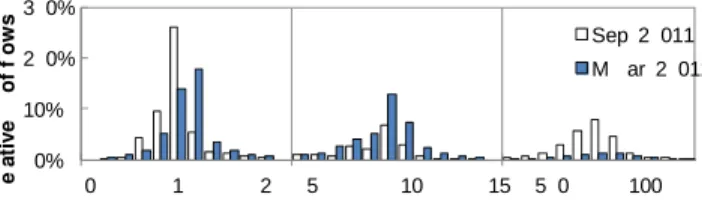
0% 10% 2 0% 3 0% 0 1 2 5 10 15 5 0 100 15 0 R e la ti v e % o f fl o w s
Estimated TCP timestamp granul arity ( ms)
Sep 2 011 M ar 2 012
Figure 3: Distribution ofG estimates.
can resolve TTFB estimates, we want to determine whether most TCP connections have a fine enough granularity. Reso-lutions from 1 to 10 ms are sufficient to differentiate changes in TTFB latencies since they are several multiples of this res-olution. By examining packet traces of several popular UE devices, we find that common timestamp granularities are 1, 5, 10, and 100 ms. Next, we estimateGfor TCP connec-tions from the network traces and plot the distribution in Figure 3. Our estimates ofGusing Equation 1 correspond to the expected granularities, though the 5 ms granularity does not appear in a significant number of connections. For both network traces, we are able to see clusters around ex-pected values ofGfrom 96% of connections. In our valida-tion below, we evaluate whether quantizing these estimated
Gvalues to 1, 5, 10, and 100 ms would result in higher ac-curacy, since other values are most likely due to estimation errors. Threfore,Gis indeed accurate in the face of actual variance in scheduling and transmission delays.
We see a shift toward finer timestamp granularity over 6 months between trace collections, which corresponds to newer devices. If this trend continues, estimation accuracy will improve.
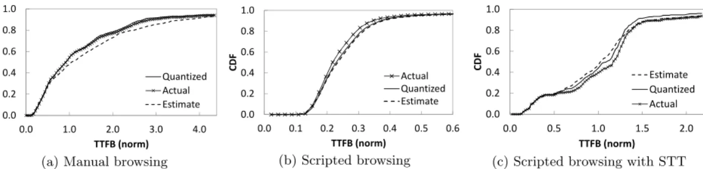
TTFB Validation. In order to determine the accuracy of our approach, we compare the TTFB estimates derived from the network traces against the actual TTFB as seen in the UE traces. Latencies from UE traces closely reflect the approach used in most popular active probing tools that ex-ecute within the Web browser or a standalone application, with the exception of the DNS exchange that we exclude. We use a UE with a 1mstimestamp granularity in three scenarios: a) manual browsing, b) scripted browsing (with-out state transitions), and c) scripted browsing with state transitions. We find similar scripted browsing results for a UE with a 100ms granularity (omitted for brevity). Sce-nario (a) consists of 731 connections to arbitrary Web sites, and (b) and (c) have 5,149 and 278 connections (respec-tively) to 26 popular Web sites (20% are mobile versions). Manual browsing connections may or may not includeST T
as the delay between page loads is arbitrary. Scripted brows-ing does not includeST T as the delay is 1 second between loads. Scripted browsing with state transitions does include
ST T induced by a 20-second delay between loads.
The CDFs of the actual and estimated TTFB are shown in Figure 4 for all three scenarios. For competitive reasons, latency values in all plots are consistently normalized by the same constant. All scenarios show that our estimate (Equa-tion 2) produces a distribu(Equa-tion of estimates fairly close to the actual TTFB. A question posed earlier is how much the estimates would improve if we quantized estimated G
values, since we know the actual timestamp granularity is usually 1 or 10 ms. To answer this question, we apply the following heuristic: when theGestimate falls in the range
Table 2: MSE for TTFB estimations. Estimate Quantized Proposed Alternative
Manual 3.95 4.86 7.05
Scripted 0.03 0.03 0.17
Scripted with STT 1.65 2.09 2.26
Table 3: Composition of TTFB (normalized).
State ST T RT T1 RT T2−Q Q
No ST 0 (0%) 0.15 (32%) 0.31 (50%) 0.08 (18%)
With ST 0.79 (68%) 0.08 (7%) 0.29 (12%) 0.15 (13%)
(0.5,1.5) ms, quantizeGto 1 ms. This range is determined empirically from Figure 3. Figure 4 shows that using this approach (labeled Quantized) provides a slightly better es-timate of TTFB. However, since the improvement is small and quantizing would result in incorrect results for fractional timestamp granularities, which are allowed, we do not use quantizing in our implementation.
The mean-squared-error (MSE) of estimates is shown in Table 2. The quantized estimate has the same error as the proposed one (Equation 2) in the scripted scenario, and a moderate advantage for other scenarios is indicated by lower MSE, as expected. For completeness, we also evaluate the alternative formulation (Equation 3) and it has higher error, especially for the scripted scenario. The error in scenarios that includeST T is moderated by the relative magnitude of
ST T that dominates total TTFB. Due to its high error, we did not implement the alternative formulation.
State Transition Validation. Finally, to validate that our FSM can approximately distinguish TTFBs with and without state transitions, we compare our FSM’s estimated transitions, which are based on the network trace, to the RNC radio event logs, which record when the UE really has a state transition.7
We find that over 76% of our estimated transitions are correct. 10% of incorrect estimates are edge cases, such as starting and ending a measurement session, while the remaining 14% are cases when signaling traffic that is not observable at the Gn keeps the UE in active state. Since the FSM classifies a large majority correctly, it is sufficient to determine whether changes in TTFB values are due to changes in theST T.
5.
DEPLOYMENT AND RESULTS
We have implemented our TTFB estimation technique in a probe platform on the production network of a major U.S. cellular carrier. In addition to performance estimation, the platform categorizes TCP flows by application, domain, and device type using HTTP signatures and GTP-C informa-tion [18]. In this secinforma-tion, we describe some early results from this deployment.
TTFB Latency Breakdown. The difference in TTFB for connections with and without a state transition is shown using CDFs in Figure 5. The averages of key constituent latencies in the TTFB, estimated using formulae in Table 1, are listed in Table 3. Both results demonstrate the large contribution ofST T to total response time.ST T comprises 68% of TTFB, on average, when a state transition occurs
7
Due to load, resource, and vendor limitations, it is not practical to collect and process RNC logs continuously [17], which is why an estimation approach is needed.
0.0 0.2 0.4 0.6 0.8 1.0 0.0 1.0 2.0 3.0 4.0 C D F TTFB (norm) Quantized Actual Estimate
(a) Manual browsing
0.0 0.2 0.4 0.6 0.8 1.0 0.0 0.1 0.2 0.3 0.4 0.5 0.6 C D F TTFB (norm) Actual Quantized Estimate (b) Scripted browsing 0.0 0.2 0.4 0.6 0.8 1.0 0.0 0.5 1.0 1.5 2.0 C D F TTFB (norm) Estimate Quantized Actual
(c) Scripted browsing with STT
Figure 4: Validation of TTFB estimates.
0.0 0.2 0.4 0.6 0.8 1.0 1.2 1.4 LTE tablet HSUPA tablet HSUPA phone HSPA+ phone HSDPA phone2 HSDPA phone HSDPA tablet La te n cy ( n o rm ) RTT TTFB TTFBwST (a) Devices 0.0 0.1 0.2 0.3 0.4 0.5 0.6 1 2 3 4 5 6 7 8 9 10 11 1 2 3
portals social nets
La te n cy ( n o rm ) RTT TTFB (b) Domains 0.0 0.1 0.2 0.3 0.4 0.5 st re am in g ap p st o re b ro w si n g g am e th u m b n ai ls h tt p o th e r ja v as cr ip t an al y ti cs b ro w si n g m ap s ja v as cr ip t p h o to ap p so ci al 1 so ci al 2 g am e 1 g am e 2 A B C D E La te n cy ( n o rm ) RTT TTFB (c) Applications
Figure 6: Comparison of mean RTT vs. mean TTFB. Error bars indicate 95% confidence intervals.
0.0 0.2 0.4 0.6 0.8 1.0 0.0 0.5 1.0 1.5 2.0 C D F TTFB (norm)
With state transition No state transition
Figure 5: TTFB with and without STT.
(Table 3). In addition, we observe that the average server delayQis non-negligible.
TTFB by Device, Domain, and Application. Next, we present three examples where TTFB offers a more com-plete picture of user experienced delay than RTT, using 51
2
hours of network data collected from 4:50PM ET on May 2, 2011. Figure 6 shows estimated RTT (as per [8]) and TTFB by device, domain, and application. Mobile devices with newer radio technology are expected to offer a better user experience, but we observe that the improvements can be subtle. Figure 6a shows that devices with HSUPA/HSPA+ have lower RTT and TTFB over those without (HSDPA), while there is no significant difference for TTFB with state transitions. However, the LTE device shows better perfor-mance across all metrics. This is due to the fact that LTE technology has both higher data rates and shorter state tran-sition delays, while both HSDPA and HSUPA/HSPA+ de-vices have the same state transition delay.
Figure 6b compares the RTT and TTFB for different Web portals and social network domains. We observe up to 72.5% difference in TTFB between domains that have nearly
iden-tical measured RTT (social networks 2 and 3). This can be mostly attributed to varying processing delays and HTTP packet transmission delays, which RTT estimates do not capture. As cellular technologies with lower transmission delay are deployed, such as LTE, server processing delay will make up a larger faction of the TTFB (Table 3).
Figure 6c shows the RTT and TTFB of different appli-cations, grouped by domain (all apps under the same letter are transactions to the same domain). We again see exam-ples where TTFB differentiates user-perceived performance but RTT does not. For example, we have cases where there is no correlation between RTT and TTFB (domains B and C). The three application classes that stand out are analyt-ics, http-other and javascript, which are served up to 36% slower than browsing and photoapp in domains B and C, respectively. The higher TTFB is likely the consequence of such transactions occurring in parallel with others.
6.
CONCLUSION AND FUTURE WORK
This paper presented an accurate and light-weight tech-nique to estimate TTFB of HTTP connections. Our early results from a deployment in a large cellular carrier demon-strate that TTFB, a large component of user response time, can vary substantially along many dimensions, even when measured RTT does not. Hence, measuring TTFB provides a more complete picture of the user experienced delay. In addition, our technique allows each component of TTFB to be studied separately, such as state transitions and server delay. While presented technique is applicable not only to cellular networks, there may be simpler methods available, depending on the transmission technologies in each particu-lar case. In the future, we plan to improve the accuracy of our state estimation FSM by including more states. We are also evaluating ways to include the DNS exchange into our definition of TTFB.
7.
REFERENCES
[1] Apache 2.2 keepalivetimeout directive.
http://httpd.apache.org/docs/2.2/mod/core.html# keepalivetimeout.
[2] For impatient web users, an eye blink is just too long to wait. http://www.nytimes.com/2012/03/01/ technology/impatient-web-users-flee-slow-loading-sites.html,
2012.
[3] J. Erman, A. Gerber, K. K. Ramadrishnan, S. Sen, and O. Spatscheck. Over the top video: The gorilla in cellular networks. InACM Internet Measurement Conference, pages 127–136. ACM, 2011.
[4] A. Gerber, J. Pang, O. Spatscheck, and
S. Venkataraman. Speed testing without speed tests: Estimating achievable download speed from passive measurements. InACM Internet Measurement Conference, pages 424–430. ACM, 2010.
[5] J. Huang, F. Qian, A. Gerber, Z. M. Mao, S. Sen, and O. Spatscheck. A close examination of performance and power characteristics of 4G LTE networks. In
ACM International Conference on Mobile Systems, Applications, and Services (MobiSys), 2012. [6] IETF. RFC 1323: TCP extensions for high
performance, supersedes RFC 1072, RFC 1185, 1992. [7] S. Jaiswal, G. Iannaccone, C. Diot, J. Kurose, and
D. Towsley. Inferring TCP connection characteristics through passive measurements. InIEEE INFOCOM, volume 3, pages 1582–1592 vol.3, 2004.
[8] H. Jiang and C. Dovrolis. Passive estimation of TCP round-trip times.SIGCOMM Comput. Commun. Rev., 32(3):75–88, 2002.
[9] S. Khirman and P. Henriksen. Relationship between quality-of-service and quality-of-experience for public Internet service. InPassive and Active Measurement Workshop, 2002.
[10] R. B. Miller. Response time in man-computer conversational transactions. InProceedings of the December 9-11, 1968, fall joint computer conference, part I, AFIPS ’68 (Fall, part I), pages 267–277, 1968. [11] J. Perez-Romero, O. Sallent, R. Agusti, and M. A.
Diaz-Guerra.Radio Resource Management Strategies in UMTS. Wiley, 1 edition, 2005.
[12] F. Qian, A. Gerber, Z. M. Mao, S. Sen, O. Spatscheck, and W. Willinger. TCP revisited: A fresh look at TCP in the wild. InACM Internet Measurement Conference, pages 76–89. ACM, 2009.
[13] F. Qian, Z. Wang, A. Gerber, Z. M. Mao, S. Sen, and O. Spatscheck. Characterizing radio resource
allocation for 3G networks. InACM Internet Measurement Conference, 2010.
[14] P. Romirer-Maierhofer, A. Coluccia, and T. Witek. On the use of TCP passive measurements for anomaly detection: A case study from an operational 3G network. In2nd COST TMA Workshop, Zurich, Switzerland, 2010.
[15] P. Romirer-Maierhofer, F. Ricciato, A. D’Alconzo, R. Franzan, and W. Karner. Network-wide
measurements of TCP RTT in 3G. InInternational Workshop on Traffic Monitoring and Analysis (TMA), pages 17–25, Berlin, Heidelberg, 2009. Springer-Verlag. [16] B. Veal, K. Li, and D. Lowenthal. New methods for
passive estimation of TCP round-trip times. In
Passive and Active Measurement Workshop, 2005. [17] Q. Xu, A. Gerber, Z. M. Mao, and J. Pang. AccuLoc:
Practical localization of performance measurement in 3G networks. InACM MobiSys, 2011.
[18] Q. Xu, A. Gerber, Z. M. Mao, J. Pang, and
S. Venkataraman. Identifying diverse usage behaviors of smartphone apps. InACM IMC, 2011.