Randomly-connected Non-Local
Conditional Random Fields
by
Mohammad Javad Shafiee
A thesis
presented to the University of Waterloo in fulfillment of the
thesis requirement for the degree of Doctor of Philosophy
in
Systems Design Engineering
Waterloo, Ontario, Canada, 2017
c
Examining Committee Membership
The following served on the Examining Committee for this thesis. The decision of the Examining Committee is by majority vote.
External Examiner Prof. Greg Mori
School of Computing Science, Simon Fraser University
Supervisor Prof. Alexander Wong
Systems Design Engineering, University of Waterloo
Supervisor Prof. Paul Fieguth
Systems Design Engineering, University of Waterloo
Internal Member Prof. Stacy Scott
Systems Design Engineering, University of Waterloo
Internal-external Member Prof. Dana Kulic
Electrical & Computer Engineering, University of Waterloo
Internal-external Member Prof. Zhou Wang
This thesis consists of material all of which I authored or co-authored: see Statement of Contributions included in the thesis. This is a true copy of the thesis, including any required final revisions, as accepted by my examiners.
Statement of Contributions
Content from 9 papers are used in this thesis. I was the co-author with major contributions on designing the methods, implementation and writing the papers:
M. J. Shafiee, A. Wong, P. Siva, and P. Fieguth, “Efficient Bayesian Inference Using Fully Connected Conditional Random Fields with Stochastic Cliques”, IEEE International Conference on Image Processing (ICIP), 2014.
This paper is incorporated in Chapter 3 of this thesis.
M. J. Shafiee, A. G. Chung, A. Wong, and P. Fieguth, “Improved fine structure modeling via guided stochastic clique formation in fully connected conditional random fields”, IEEE International Conference on Image Processing (ICIP), 2015.
This paper is incorporated in Chapter4 of this thesis.
M. J. Shafiee, A. Wong, and P. Fieguth, “Deep Randomly-connected Conditional Ran-dom Fields For Image Segmentation”, IEEE Access Journal, 2016.
This paper is incorporated in Chapter4 and 5 of this thesis.
M. J. Shafiee, A. Wong, and P. Fieguth, “Forming A Random Field via Stochastic Cliques: From Random Graphs to Fully Connected Random Fields”, arXiv:1506.09110, 2015.
This paper is incorporated in Chapter 6.
M. J. Shafiee, P. Siva, and A. Wong, “Stochasticnet: Forming deep neural networks via stochastic connectivity”, IEEE Access Journal, 2016.
M. J. Shafiee, P. Siva, P. Fieguth, and A. Wong, “Efficient Deep Feature Learning and Extraction via StochasticNets”, IEEE Computer Vision and Pattern Recognition Work-shops (CVPRW), 2016.
This paper is incorporated in Chapter 6.
M. J. Shafiee, P. Siva, C. Scharfenberger, P. Fieguth, and A. Wong, “NeRD: A Neural Response Divergence Approach to Visual Saliency Detection”, IEEE Signal Processing Letters (SPL), 2016.
This paper is incorporated in Chapter 6.
M. J. Shafiee, P. Siva, P. Fieguth, and A. Wong, “Embedded Motion Detection via Neural Response Mixture Background Modeling”, IEEE Computer Vision and Pattern Recognition Workshops (CVPRW), 2016.
This paper is incorporated in Chapter6.
M. J. Shafiee, and A. Wong, “Evolutionary Synthesis of Deep Neural Networks via Synap-tic Cluster-driven GeneSynap-tic Encoding”, Neural Information Processing Systems Workshops (NIPS), 2016. Best paper award.
Abstract
Structural data modeling is an important field of research. Structural data are the combi-nation of latent variables being related to each other. The incorporation of these relations in modeling and taking advantage of those to have a robust estimation is an open field of research. There are several approaches that involve these relations such as Markov chain models or random field frameworks. Random fields specify the relations among random variables in the context of probability distributions. Markov random fields are generative models used to represent the prior distribution among random variables. On the other hand, conditional random fields (CRFs) are known as discriminative models computing the posterior probability of random variables given observations directly.
CRFs are one of the most powerful frameworks in image modeling. However practical CRFs typically have edges only between nearby nodes. Utilizing more interactions and expressive relations among nodes make these methods impractical for large-scale applica-tions, due to the high computational complexity. Nevertheless, studies have demonstrated that obtaining long-range interactions in the modeling improves the modeling accuracy and addresses the short-boundary bias problem to some extent. Recent work has shown that fully connected CRFs can be tractable by defining specific potential functions. Although the proposed frameworks present algorithms to efficiently manage the fully connected in-teractions/relatively dense random fields, there exists the unanswered question that fully connected interactions are usually useful in modeling. To the best of our knowledge, no research has been conducted to answer this question and the focus of research was to introduce a tractable approach to utilize all connectivity interactions.
This research aims to analyze this question and attempts to provide an answer. It demonstrates that how long-range of connections might be useful. Motivated by the an-swer of this question, a novel framework to tackle the computational complexity of a fully connected random fields without requiring specific potential functions is proposed. In-spired by random graph theory and sampling methods, this thesis introduces a new clique structure called stochastic cliques. The stochastic cliques specify the range of effective connections dynamically which converts a conditional random field (CRF) to a
randomly-connected CRF. The randomly-randomly-connected CRF (RCRF) is a marriage between random graphs and random fields, benefiting from the advantages of fully connected graphs while maintaining computational tractability. To address the limitations of RCRF, the pro-posed stochastic clique structure is utilized in a deep structural approach (deep structure randomly-connected conditional random field (DRCRF)) where various range of connec-tivities are obtained in a hierarchical framework to maintain the computational complexity while utilizing long-range interactions.
In this thesis the concept of randomly-connected non-local conditional random fields is explored to address the smoothness issues of local random fields. To demonstrate the effectiveness of the proposed approaches, they are compared with state-of-the-art methods on interactive image segmentation problem. A comprehensive analysis is done via different datasets with noiseless and noisy situations. The results shows that the proposed method can compete with state-of-the-art algorithms on the interactive image segmentation prob-lem.
Acknowledgments
I would like to express my gratitude to my two co-supervisors, professors Alexander Wong and Paul Fieguth for their tremendous supports and guidance on my development as a scientist and a researcher. Prof. Wong thank you for involving me in different research and industrial projects while guiding me in the right direction, encouraging me to explore different ideas and helping me shape them properly; most important of all, thanks for giving me the insight that research is fun. Prof. Fieguth thank you for your meticulous comments on how to develop the ideas and the elucidation of several different topics. I learnt how to formulate my problems mathematically which helped me provide strong theory to back my experiments. Thank you both, you taught me there is no fear in research, just need to have faith, dive in and be persistent.
I would sincerely like to thank my Ph.D. committee members Prof. Stacy Scott from Systems Design Engineering department, Prof. Dana Kulic and Prof. Zhou Wang from Electrical and Computer Engineering department for their time and commitment. I also would like to thank Prof. Greg Mori from School of Computing Science, Simon Fraser University for his time to accept reviewing the thesis.
Many thanks to my colleagues in Vision and image Processing Research Group at University of Waterloo, for always being helpful and bring the productivity atmosphere into the lab.
Special thanks to my friends Hamed (Dr. Shahsavan), Mohammad (Dr. Mohammadi) and Amir-Hossien (to be Dr. Karimi in future years) for cheering me up during the lows and highs, no matter I was down in the dumps or jumped for a joy (the Ph.D. life situations)!
Finally but the most importantly, I would like to thank my family for their huge sup-ports and encouragement. To my beloved parents for always encouraging me to pursue the academic pathway and their non-stop supports, to my sister and brothers for their enthusiasm in my success and their encouragement in defeat.
Dedication
To my beloved parents, My dear sister and brothers,
Table of Contents
List of Tables xiv
List of Figures xv
Nomenclature xvii
1 Introduction 1
1.1 Problem Definition . . . 2
1.2 Challenges and Objective. . . 3
1.3 Contribution. . . 5
1.4 Thesis Structure. . . 6
2 Background & Related Work 7 2.1 Graphical Models . . . 8
2.2 Probabilistic Models . . . 11
2.2.1 Generative Models . . . 12
2.2.2 Discriminative Models . . . 13
2.3.1 Clique Structures . . . 16
2.3.2 Random Graphs . . . 19
2.4 Conditional Random Fields . . . 20
2.4.1 Local Random Fields . . . 24
2.4.2 Hierarchical Random Fields . . . 25
2.4.3 Fully Connected Random Fields . . . 27
2.5 Efficient Inference Approach . . . 29
2.5.1 Permutohedral Lattice Based Method . . . 29
2.5.2 FFT Based Method . . . 31
2.5.3 Related Methods . . . 33
2.6 Deep Conditional Random Fields . . . 36
2.7 Summary . . . 38
3 Randomly-Connected Random Fields 40 3.1 Introduction . . . 41
3.2 Problem Definition . . . 42
3.3 Randomly-Connected Conditional Random Fields . . . 48
3.3.1 Stochastic Cliques . . . 50
3.3.2 Graph Representation . . . 52
3.4 Inference . . . 54
3.4.1 Graph Cut . . . 55
3.5 Example Problem . . . 56
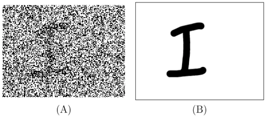
3.5.1 Binary Image Classification . . . 57
4 Deep Randomly-connected Conditional Random Field 61
4.1 Introduction . . . 62
4.2 Deep Structures . . . 63
4.3 Deep Randomly-connected Conditional Random Fields . . . 65
4.4 DRCRF Methodology . . . 68 4.4.1 Graph Representation . . . 71 4.4.2 MAP Inference . . . 73 4.5 DRCRF Layer-wise Analysis . . . 74 4.6 Summary . . . 75 5 Experimental Results 78 5.1 Introduction . . . 79 5.1.1 Dataset Description . . . 79 5.1.2 Competing Algorithms . . . 81 5.2 Model Configuration . . . 82 5.2.1 Parameter Description . . . 82 5.2.2 Unary Potential . . . 83 5.3 Quantitative Evaluation . . . 84 5.3.1 Quantitative Measures . . . 84
5.3.2 Connectivity Range Effect on RCRF . . . 85
5.3.3 Connectivity Range Effect on DRCRF . . . 87
5.3.4 Noiseless Images . . . 88
5.3.5 Noisy Images . . . 90
5.4 Qualitative Evaluation . . . 92
5.5 Summary . . . 103
6 Conclusion & Future Work 107 6.1 Thesis Contribution Highlights. . . 108
6.1.1 Limitations . . . 110
6.2 Future Work . . . 111
6.2.1 Mathematical Hypothesis . . . 111
6.2.2 Connectivity Computation via Abstraction . . . 112
6.2.3 Graphical Models & Deep Learning Approaches . . . 115
List of Tables
3.1 Quantitative results based on the EnglishHnd datase . . . 59
5.1 Region F1-score results in a noiseless context for all Datsets . . . 89
5.2 Boundary F1-score results for all four datasets in noise free context . . . . 89
5.3 Intersection Over Union (IOU) results in noise free situation. . . 90
5.4 Region F1-score results for noisy cases . . . 91
5.5 Boundary F1-score results for noisy cases . . . 91
5.6 Intersection Over Union (IOU) results for noisy images. . . 91
List of Figures
2.1 HMM vs Kalman graphical model . . . 8
2.2 First order Markov connectivity . . . 17
2.3 First order Markov clique structures. . . 18
2.4 Second order Markov clique structures . . . 18
2.5 Adjacency CRF graphical model. . . 23
2.6 Fully connected conditional random fields. . . 28
3.1 Problem Definition Flow-diagram . . . 44
3.2 Binary image classification sample . . . 47
3.3 Accuracy per number of interactions . . . 48
3.4 Multi-label image classification . . . 49
3.5 Accuracy per number of interactions in a non-local problem . . . 50
3.6 RCRF graph visualization . . . 53
3.7 Qualitative results of RCRF of EnglishHnd datase . . . 58
4.1 Interactive image segmentation example . . . 67
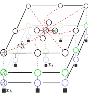
4.2 deep randomly-connected conditional random field graph . . . 72
5.1 Weizmann Dataset Exapmle Images . . . 79
5.2 CSSD Dataset Exapmle Images . . . 80
5.3 MRIS Dataset Exapmle Images . . . 80
5.4 The effect of γ on modeling accuracy . . . 86
5.5 Quantitative analysis of σ on the performance of a two-layer DRCRF. . . . 88
5.6 Performance comparison based on various noise power . . . 93
5.7 Qulitative results on Weizmman datasets . . . 95
5.8 Qualitative result– Airplane examples . . . 96
5.9 Qualitative result– Bird examples . . . 97
5.10 Example segmentation results for CSSD and MRIS datsets . . . 98
5.11 Qulitative comparison– Reclying girl . . . 99
5.12 Qulititave example– Two men . . . 100
5.13 Qulitative comparison via elongated object . . . 101
5.14 Example segmentation results of noisy images . . . 102
5.15 Example segmentation results for an object with elongated boundaries . . 104
5.16 Example noisy segmentation– Twon hall . . . 105
5.17 Segmentation example of a noisy image . . . 106
Nomenclature
Randomly-connected random Field γ Sparsity factor
σp Controling paramter
σq Controling paramter
L Number of layers
Pi,js Spatial probability
Qdi,j Color similarity probability Random Field
ˆ
Yt Sub-optimal result at layer t E(·) Expectation
C Clique structures
St Graph cut at layer t
ω Weigth of feature fucntion
ψp(·) Pairwise potentials
ψu(·) Unary potentials
θ The set of weights
ϕ A clique
Cp(i) The set of pairwise cliques corresponding to node i
D(·) KL-divergence E(·) Energy function
xi Measurement of node i
Y Probabilistic model, Random field
Y? The optimal result
yi Associated random variable to node i
Z Normalization constant
Graph
E The set of edges in graph
V The set of nodes in graph eij Edge between nodes i and j
G Undelying graph
n Number of nodes
ui The coordinates of node i
Chapter 1
Introduction
Graphical models [84,170] are one of the most important field of statistical machine learn-ing which try to encode the statistical computational models deallearn-ing with structural data via a graph representation. The random variables are represented by nodes and the in-teractions among them are visualized via weighted edges in the graph. Nowadays, several fields of machine learning such as computer vision [13, 89], speech recognition [53, 129] and natural language processing [28] utilize graphical models to formulate and solve prob-lems. Computer vision due to dealing with images is the field with most usage of graphical models specially random fields [13,45, 96].
Computer vision applications have been usually proposed to provide a solution to natu-ral images such as human body images [4,107] (MRI, OCT) or natural scenes [94,150] and man-made objects. The most important intrinsic property of those images is the relations among pixels in the image, specially when the pixels are close to each other. This property implies that neighbor pixels should have same color intensity. Due this fact, probabilistic graphical models have been trying to take advantage of this property and to address various type of problems [65, 128]. Incorporating different size of interactions is the focus in this challenge [89] and researchers have been trying to provide more interactions in their models by introducing tractable approaches. This research aim at stepping toward analyzing those approaches and answers the question that there is any way to determine how to configure
the underlying graph representation of a graphical model to produce an optimal model. Here we restrict our focus to conditional random fields (CRFs) [80, 98] and we study the effect of long-range non-local connectivity in modeling accuracy. Motivated by the answer of the question, we propose an efficient framework to address the computational complexity in the inference step of long-range non-local random field models. In this dissertation, the idea of randomly-connected non-local conditional random fields is explored to address the aforementioned issues of local random fields.
1.1
Problem Definition
Probabilistic graphical models are the way to visualize probabilistic models which ease the understanding of these models, unify and generalize them in the context of graph theory. Random fields are a type of graphical models utilized to model 2-D problems such as computer vision applications [89, 96, 185]. Random fields model the problem by taking advantage of the relations among different pixels in the image. Each pixel or super-pixel is represented by a random variable in the random field and it models the image by computing the relations among the random variables. Those relations are expressed as energy over the random field. Based on the Gibbs theory [45] the energy propagates in the random field to reach an equilibrium state. The relations among random variables are simulated by the Gibbs energy and the estimation is obtained by finding the equilibrium over the random field.
Conventionally, local interactions are applied to define the energy function. This is because of computational complexity of inference step. The computational complexity is increased by adding more interactions in the model and it has quadratic relation with the number of interactions. The ability of the local CRFs1 is limited to model long-range connections and generally leads to excessive smoothing of object boundaries.
1We use the terms of “random field” and “conditional random field” sometimes in the text
interchange-ably. Although the main focus of this thesis is on CRF models, it is possible to extend all algorithms to other types of random fields as well.
In order to improve modeling accuracy and providing the longer-range of connections, researchers have expanded the local framework to incorporate hierarchical connectivity and higher-order potentials [43, 65, 94] defined on image regions. Unsupervised image segmentation usually provides the higher order connectivity structure in the majority of these frameworks. Although these approaches incorporated higher order connectivity in modeling, their accuracy is necessarily restricted by the effectiveness of unsupervised image segmentation.
Global connectivities can prevent smoothness in inference and labeling step. In addi-tion, fully connected random fields can encode both color contrasts and spatial arrange-ments of different nodes by edge potentials instead of grid random field (locally random fields) where the edges only serve the contrast sensitive smoothness. Therefore, new re-searches have been conducted to address this problem recently [89,185].
Although the proposed frameworks [89, 185] presented algorithms to manage the fully connected interactions, there exists a question that fully connected interactions are always useful in modeling. To the best of our knowledge, no research has been conducted to answer this question and the focus of researches was to introduce a tractable approach to utilize all connectivity interactions. Here we aim to take advantage of random graph theory and model the dense and non-local random fields via a stochastic process. By use of this approach, the underlying dense graph of random field is modeled by a sparse graph which addresses the computational complexity of the inference to some extent.
1.2
Challenges and Objective
Despite the fact that several methods and algorithms have been proposed to tackle different aspects of long-range non-local random fields, it is still considered as an open-field of research and there are many unanswered questions in this area yet. Although it has been shown that the long-range non-local random fields can improve the modeling accuracy compared to local random fields, generating the long-range interactions in the underlying graph and also managing the computational complexity of the new model are still the big
challenges of these approaches:
• Although it has been shown that fully-connected random fields improve modeling accuracy in several problems, there is no comprehensive answer to the question that how many connections are needed to have an accurate model.
• Increasing the number of interactions in the random field modeling has a significant effect on computational complexity, therefore proposing a strategy to make a trade-off between modeling accuracy and computational complexity is another challenge in this field.
Several algorithms have been conducted to tackle the aforementioned challenges either addressing only one aspect or proposing a method to solve them simultaneously. These methods can be divided in different categories depends on their focus in formulating the problem which mainly are proposing new penalty functions, reformulating the potential functions to reduce the computational complexity and applying higher order cliques or longer-range of connectivities via a less computational complexity burden framework. The first and second categories usually are associated with some limitations. Here in this dissertation, our main objective is to tackle the aforementioned challenges via the third category and we follow these objectives through this thesis:
• As the first objective, we will study whether utilizing larger number of long-range connectivities always helps to improve the modeling accuracy or not. We will demon-strate the advantages and disadvantages of longer-range of connectives via different examples.
• Motivated by those examples, the main objective will be a new representation for the underlying graph of random fields such that while it utilizes the long-range con-nectivities it maintains the computational complexity as well.
• It has been shown that hierarchical models have the ability to capture global and local information in modeling random fields in several problems. As the last objective,
we aim to take advantage of hierarchical models to obtain more useful information combined with the achievement of the second objective to model the underlying graph of random fields more efficiently and accurately.
The proposed methods based on the above objectives will be examined within the context of interactive object segmentation problem and they will be analyzed in terms of performance and behavioral in random fields modeling.
1.3
Contribution
The described objectives in this research lead to the following contributions:
• Proposing a new clique structure, stochastic clique, [146] which is the marriage of random graph theory and random field theory. The stochastic clique structure takes advantage of long-range connectivities via random graph theory within a stochastic process. The stochastic process determines which set of cliques are more informative in the inference step.
• Randomly-connected conditional random field (RCRF) [139,146]; applying the stochas-tic clique structure into the random field modeling leads to a new representation for the long-range non-local random fields which the interactions among nodes are ran-domly determined and as the result, the structure of underlying graph is random. The proposed RCRF model creates a random field where only the most useful long-range and non-local interactions are incorporated in the modeling. The computational complexity of modeling procedure is maintained while long-range connections are involved in the modeling using this approach.
• Deep structure randomly-connected conditional random field (DRCRF) [145]; incor-porating stochastic cliques makes the use of non-local and long-range connectivities applicable, however there is a limitation to the number of interactions which is mostly related to the inference algorithm. Although utilizing stochastic cliques decreases the
number of active cliques in the inference step, inference methods are not capable of maintains huge number of connectivities in the random field modeling yet. To ad-dress this problem, we aim to apply a deep structure model which utilizes a subset of connectivities in each level of hierarchy and it helps the inference method to be able to handle the inference process easily.
All the described contributions are combined together at the end to work as a unique framework to model the problem via the context of non-local and long-range random field.
1.4
Thesis Structure
This thesis is organized in six chapters. Chapter2introduces graphical models and various type of random fields. This chapter provides a mathematical definition for random fields specially discriminative model and conditional random fields. Then, an overview of fully connected random fields and proposed tractable approaches are presented. In Chapter 3 we analyze the effect of long-range interactions in random field modeling for different set of simulated examples. Motivated by those examples, we introduce the concept of stochastic cliques and we propose randomly-connected conditional random field model. Our proposed deep structure randomly-connected conditional random field is explained in Chapter 4 and we analyze its behavioral in this chapter. We examine the proposed methods along with several state-of-the art approaches in Chapter5and we evaluate them in different situations. Finally, thesis is concluded in chapter 6 and future directions for this dissertation are provided at the end.
Chapter 2
Background & Related Work
“Graphical models are a marriage between probability theory and graph theory. They provide a natural tool for dealing with two problems that occur throughout applied mathematics and engineering – uncertainty and complexity – and in particular they are playing an increasingly important role in the design and analysis of machine learning algorithms. Fundamental to the idea of a graphical model is the notion of modularity – a complex system is built by combining simpler parts. Probability theory provides the glue whereby the parts are combined, ensuring that the system as a whole is consistent, and providing ways to interface models to data. The graph theoretic side of graphical models provides both an intuitively appealing interface by which humans can model highly-interacting sets of variables as well as a data structure that lends itself naturally to the design of efficient general-purpose algorithms.”
2.1
Graphical Models
Probabilistic graphical models [74,84,170] are powerful tools to combine graph theory and probability theory in a unified formalism for statistical multivariate problems. Probabilistic graphical models (usually called graphical models) are utilized to represent probabilistic models in a visual way to make them easier to interpret. There are several probabilistic models such as hidden Markov models (HMMs) [128], Markov random fields [27, 40, 104], Kalman filters [40,175] and Bayesian networks [10,161] which have been utilized in different applications. The role of a graphical model is to ease the understanding of these models, to unify them and to generalize them in the context of graph theory. For instance, HMMs and Kalman filters can be described with a common graphical model (Figure2.1). A graphical model is a natural tool to formulate the variations of these classical models, especially when a large numbers of interacting variables are being studied together.
Graphical models are the combination of probabilistic models and graph theory. Graph theory plays an important role as a language to formulate probabilistic models. Further-more, it is a useful tool to express computational complexity and feasibility when designing a model. In particular, the running time of an algorithm or the magnitude of an error bound can often be characterized in terms of structural properties of a graph.
A graph G = (V,E) is formed as a collection of vertices V ={v1, v2, . . . , vm} and the
(a) (b)
Figure 2.1: The graphical model realization of a HMM and a Kalman filter. The difference between (a) the HMM and (b) the Kalman filter is that the number of statesyi is indefinite
in the Kalman filter while it is finite in HMM. xi represents the measurement at time i
set of edges E ⊆ V × V where each edge is encoded via a pair of vertices {vi, vj} ∈ V (its
two end nodes). The edgeeij may be undirected or directed, such that edge (vi → vj) is
different from (vj →vi) in directed graphs.
Each random variableyi of a probabilistic model Y ={y1, y2,· · · , yn}is represented as
a node vi ∈ V. The dependency between two random variables yi and yj is expressed by
the edge eij or eji when it is modeled by a directed graph. The first subscript represents
the starting point (parent node) while the second one shows the ending point (child node). The edges eij and eji are identical since there is no direction in an undirected graph.
There are causal relations among variables in applications such as temporal problems. For example when you want to predict the weather condition based on some previous days, you have a set of random variables yt that are dependent on each other and the condition
of a new day yt+1 is a consequence of previous days y1:t. Therefore, in such applications
the interactions among random variables must be characterized by direct relations, such that the state of the new day is a child of earlier ones. The directed graphical model is the target for these types of applications since there are causal interactions among the random variables. Hidden Markov models [128] and other types of Bayesian networks [161] are examples of directed graphical models.
Mathematically speaking, a graphical model is a collection of marginal probability distributions factorized according to the underlying structure of the graph. The key idea in the graphical model is the factorization that will be explained more in Sections 2.2, 2.3 and 2.4. For a directed graphical model, P(Y) can be computed based on the chain rule where each variable is marginalized given its ancestors (parent) variables (nodes):
P(Y) =P(y1, y2, . . . , yn) =P(y1|y2, . . . , yn)·P(y2|y3, . . . , yn)· . . . ·P(yn) (2.1)
the set of all random variables is shown by Y and n = |Y| is the number of random variables. To reduce the complexity of (2.1), Markov assumption is usually applied. The-oretically speaking (i.e., statistical definition) Markov assumption refers to the property of conditional probability distribution of future states of the process depends only on the present state or the limited number of past states. Based on this definition each random
variable can be modeled given a specific amount of information from the past:
P(yt+1|Y) = P(yt+1|yt) (2.2)
here it is assumed the future state of yt+1 only depends on the preset. Incorporating the Markov assumption (Section2.3.1), the marginal probability of each variableyigiven other
variables can be formulated as
P(yi|Y) =P(yi|yπ(i)) (2.3) where random variableyi ∈Y andyπ(i) ⊂Y is the set of parental nodes for random variable yi. In other words, yπ(i) determines the set of random variables that node i is dependent on. Substituting (2.3) into (2.1), the joint probability distribution of all random variables can be factorized in the following way
P(y1, y2, . . . , yn) =P(Y) = n
Y
i=1
P(yi|yπ(i)). (2.4) There are several applications such as image modeling where no specific causality among the random variables can be determined. Each pixel or super-pixel (Section 2.4.1) is modeled by a random variable. Since there does not exist any causal relation among the pixels (nodes) in the image, it is not possible to specify any direction between two nodes (i.e., edge direction) or random variables in those applications. Therefore, undirected graphical models are the best choice of modeling in such applications. Based on the Markovianity assumption, the probability distribution is factorized via a set of functions defined via the parent nodes of each random variables and the conditional independence assumption that will be explained in Section2.3.1.
The probability distribution of an undirected graphical model is factorized via a set of functionsψ(yc) :Rd→R+ P(y1, y2, . . . , ym) = 1 Z Y c∈C ψ(yc) (2.5)
whereyc is a sub-set of random variables which are connected based on the Markovianity
property of the graph. Function ψ(·) must be non-negative and it is called potential func-tion. ParameterZ is a normalization constant to enforce the output value as a probability (i.e.,P(y1, y2, . . . , ym)∈[0,1]), sinceψ(·) can be any non-negative arbitrary function. The
normalization constantZ is the summation over all configurations to represent the output value as a probability.
In summary, there are two most common types of graphical models: Bayesian networks (or belief network) [11, 161] and Markov networks (or Markov random fields) [14, 45,
172]. The former ones are represented by directed graphs while the latter ones are mostly visualized via undirected graphs.
Over all mentioned types of network structures, computational complexity is an im-portant aspect in the graphical model approaches [85]. The goal of modeling usually is to find the joint distribution P(·) over a some set of random variables. Let us assume that the variables are binary-valued and there are n variables, therefore, a joint distribu-tion requires the specificadistribu-tion of 2n numbers of different assignments of values. However,
there are some relational structures among random variables and they can be illustrated in the factorization step (2.5) which reduces the required number of calculations. The conditional independence property can be utilized to represent such high-dimensional dis-tributions much more compactly. The marginal probability of each random variable is only represented by conditioning on its neighbors, therefore, there is no need to compute all interactions.
2.2
Probabilistic Models
For many applications in machine learning the problem is to predict the value of a vector Y given the value of a vector X of input features [12]. Most machine learning applications are divided into classification and regression [11]. In classification applications,Y is single variable which is expressed by a discrete class label, whereas in a regression problem it corresponds to one or more continuous variables.
The goal of probabilistic models is to find P(Y|X). There are two different ap-proaches [11] to formulate P(Y|X):
• Direct solution to this problem is to represent the conditional distribution using a parametric model. The model must be trained to find the required parameters based on training set consisting pairs of {X, Y}. The trained model can be used to predict Y for a new input vectorX. These types of methods are called discriminative models since they discriminate directly between the different values of Y.
• Joint distribution of P(Y, X) is counted as the second approach. The joint distribu-tion is utilized to evaluate the condidistribu-tional probability P(Y|X) implicitly in order to make predictions of Y for new values of X. This is known as a generative approach since by sampling from the joint distribution it is possible to generate synthetic ex-amples of the feature vector X.
The following sections explain these two frameworks with more details.
2.2.1
Generative Models
In the context of probability and statistics, generative models [74, 33] are a type of prob-abilistic model that can generate synthetic examples randomly given hidden parameters Y. As mentioned before, a generative model specifies the joint probability distribution of observation and hidden states (i.e., labels or class) while the conditional probability of states given observations is formed via Bayes’ rule. Although generative models obtain the conditional probability of states given observations by use of the joint probability, an assumption needs to be made to be able to compute the conditional probability. Bayes’ rule states that:
P(Y, X) = P(X|Y)P(Y) (2.6)
whereP(X|Y) is the likelihood model andP(Y) is the prior one. The exact computation of the likelihood models is usually intractable, therefore, a conditional independence assump-tion [80] is taken into account to make the likelihood model tractable. The conditional
independence assumption assumes that each observation is independent from other obser-vations given its state. Mathematically speaking, the likelihood model is approximated as the product of independent probabilities given the conditional independence assumption,
P(X|Y) =
N
Y
i=1
P(xi|yi), |X|=N. (2.7)
However natural data are usually high dimensional and several dimensions are corre-lated [40], therefore, the conditional independence assumption on X is not a proper as-sumption to make. Thus the modeling accuracy of generative models created by this assumption is lower than discriminative model [12] since the discriminative model provides a direct conditional probability.
Although generative models have some drawbacks compared to discriminative ap-proaches in modeling accuracy, they have some advantages as well [164]:
• The generative model can handle missing data since the data are modeled for each class separately. This model can augment small set of labeled data with a large set of unlabeled data when the labeled data are expensive.
• A new class of data easily can be incremented to the whole classification problem since the data are modeled class dependently.
Discriminative models are preferable versus generative ones when dealing with classification problems, according to the reason asserted by Vapnik [165], the problem should be solved directly rather than be solved by the general formulation and computing the likelihood model.
2.2.2
Discriminative Models
Discriminative approaches model the problem as a conditional probability of statesY or un-seen variables given observationsX directly. The common applications of machine learning are classifications or regressions, therefore, it is more proper to model the problem directly
(P(Y|X)) rather than using joint probability distribution (i.e.,P(Y, X)). As mentioned in the last section, it is assumed that observations, X, are conditionally independent given the states, Y, to compute the likelihood model in the generative model. Therefore, the generalization performance of discriminative models is more than generative ones due the differences between the model and the true distribution of the data [12], in practice.
Generative models were more common before the advent of the maximum entropy models (MEM) [80]. The main problem of discriminative models was a way to represent the parametric form of these models. MEM asserts that the only unbiased distribution given the incomplete available data is the one that maximizes the conditional entropy of states given observations. Based on MEM, the probabilistic discriminative models are usually represented as a factorization of exponential family functions1 [80].
In other words, MEM is based on the Principle of Maximum Entropy [72] stating that the only unbiased assumption can be made to define a conditional distribution is that the distribution is as uniform as possible given the available information when information regarding the probability distribution is incomplete [80].
Two advantages of discriminative models are:
• Discriminative models are faster [84,164] than generative ones since they predict the new data point directly instead of an iterative procedure to find probability of the data point given each class.
• It is expected that discriminative methods have better predictive performance than generative approaches [84,164] because discriminative models are trained to predict the class label rather than the joint distribution of input vectors and targets.
Although our main focus here is the general representation of a graphical model, the experimental results have been done in the context of discriminative frameworks specially conditional random fields. Following sections present two well-known graphical models:
1The general formulation of MEM and conditional random fields (discriminative probabilistic models)
Markov random fields (MRFs) known as a generative model and conditional random fields (CRFs) which are one of the well-know discriminative models.
2.3
Markov Random Fields
Markov random fields (MRFs) or Markov networks [40,45,78] are a set of random variables having the Markov characteristic based on an undirected graph. The foundation of Markov random field theory came from statistical physics [78]. Each random variable is represented as a node in an undirected graph and dependencies between random variables are expressed by an undirected edge.
MRFs are generative models [172] since they are usually utilized to model the prior part of generative models. They are usually based on the notion of conditional independence and Gibbs theory; the probability distribution is formulated as a factorization of an energy function (2.5). The energy function is the combination of feature functions (2.9) specifying the relations among random variables.
Since these models are not associated with a topological ordering, it is not possible to apply chain rule to expandP(Y). Instead a potential function or a factorization is utilized to formulateP(Y) upon the maximal cliques. A potential function can be any non-negative function of its arguments. The joint distribution is then defined to be proportional to the product of clique potentials. Since exponential functions have non-negative manner, the potential functions in MRF are usually formulated in the context of exponential equation which the exponent of the formulation is called energy function. This type of expansion derives the MRF model to equate with Gibbs distribution [112]. Hammersley-Clifford [57] has been proved that the Gibbs distribution is equal to the MRF model.
In other words, the conditional independence assumption is characterized by the cliques on the represented graph. The probability distribution is formulated as a factorization of
energy function based on clique structures: P(Y) = 1 Z exp(−E(Y, θ)) (2.8) E(Y, θ) =X c∈C ψ(yc, θc) (2.9)
where c is a clique template in the set of clique structures C, θ determines the weight of each potential function ψ(·) to construct energy function E(·) and Z is the normaliza-tion constant which is the summanormaliza-tion over all configuranormaliza-tions. Finding the most probable configuration based on the MRF, is to minimize the energy functionE(·).
It is worth to mention that since the proposed framework has been applied within a conditional random field model, MRFs are not our main focused and we just explained it in a very short description here.
2.3.1
Clique Structures
Generally, a clique [110] is a subset of vertices vc ⊂ V of graph G(V,E), where V is the
vertex-set and E is the set of edges of the graph G. The sub-set vc is a fully connected
undirected graph:
vc=
vi|∀(vi, vj)∈vc, vi neighbor vj . (2.10)
Although cliques have a long history in graph theory [50,55], it is a well-known termi-nology to define a random field model as well. The connectivity and relation among nodes in a random field is defined according to the neighborhood size (i.e., Markov order) to have a tractable inference approach in an undirected graphical model. The number of cliques and the shape of them are determined by the neighborhood size. Cliques are specified by their sizes and orientations. The position of a clique in the random field is another property which characterizes it as well.
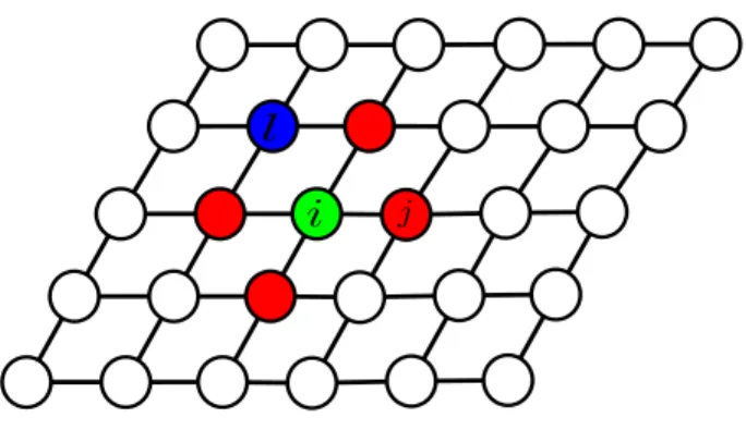
The first-order Markov assumption is a common neighborhood size. Each node in the random field is connected to the nearest four other nodes in the graph. As seen in
Figure 2.2: Each nodevj (red) is the neighbor of nodevi (green) via the first-order Markov
assumption. Node vl is not explicitly the neighbor of node vi.
Figure 2.2, the green node vi is in relation with four red nodes such as vj. The relation
between node vi and vl is not considered explicitly in the random field by the first-order
Markov assumption.
Figure 2.3 demonstrates the clique structures for the first-order Markov connectivity. As seen in Figure 2.3 (b), the connectivity in each orientation is specified by a distinct clique. Each node neighbors with eight closest nodes based on the second-order Markov connectivity. Figure 2.4 shows cliques based on the second-order Markov connectivity.
There are two assumptions [32] to merge different cliques into a same category:
• Homogeneous assumption: if the identically oriented cliques are the same in the whole random field.
• Isotropic assumption: if all orientations of a specific size of clique (i.e., number of nodes in a clique) are identical.
Our first contribution is to present a new type of clique structure to tackle the compu-tational complexity of fully connected networks. Inspired by random graph theory [16,24], the proposed clique structure takes advantage of a randomness among variables’ interac-tions to reduce the computational complexity of the inference step.
(a) (b)
Figure 2.3: Clique structures for the first-order Markov neighbors. (a) shows a four neigh-borhood connectivity and (b) demonstrates all clique structures related to the first-order Markov connectivity. There are five different clique structures based on the size and the orientations of cliques. A clique is a complete graph and based on the definition (3.4), all nodes in the cliques must be connected to each other. As a result, the maximum size of a clique is two when the random fields is defined based on four neighborhood size. It is obvious that if we assume we have maximal clique of greater than 2 ( e.g. 3) there is at least a node which is not connected to the interested node and, therefore, the maximal clique is two.
(a) (b)
Figure 2.4: Clique structures corresponding to the second-order Markov neighbors. (a) shows the second-order Markov neighbor connectivity and (b) demonstrates all possi-ble clique structures. As seen in (a), the maximal subgraph which all nodes are connected to the interested node is with four nodes, therefore, the maximal clique is four while the maximal clique in Figure2.3 was two.
2.3.2
Random Graphs
Random graph theory [16, 34, 69, 183] defines graphs based on a probability distribution which a graph is generated via a probability distribution defined over the graph. This theory is a marriage between graph theory and probability theory. A random graph is obtained by starting withn isolated vertices that will be connected at random, iteratively.
There are several studies and approaches to generate a random graph. Gilbert [16] denoted the graph asG(n, p) such that each edge connectivity is determined independently based on the probabilityp. Erd¨os–R´enyi model [24] represents the graph asG(n, m) where m determines the number of connected edges of the graph. The selection probability is calculated such that it provides the exactmedges for the graph. The Erd¨os–R´enyi model is an effective model for extracting the essential behaviors of various graph properties which are explained in this section. We define a random graph as Gn,p wheren is the number of
nodes andp represents the connection probability.
The generated random graph illustrates specific structure [24] based on the range ofp2:
• Gn,p is the disjoint union of trees if p=o(n1) where3
f(x) = og(x) iff |f(x)|< |g(x)| ∀x≥x0 , ∈R+
• Gn,p contains cycles with different sizes if p ∼ nc for 0 < c < 1. All connected
components are either trees or unicyclic components and almost all nodes (n−o(n)) are in components that are trees.
• There is an amazing fact that Gn,p is dramatically different when p < n1 from when
p > 1
n. The largest component has sizeO(logn) for the former one, while most of the
small components merge to a giant component with the size O(n). The remaining components are of size O(logn). It is called double jump when p∼ 1
n+ µ n.
2We are only using these properties and the mathematical backgrounds of them are not the concern of
this thesis, therefore, we accept them as facts.
3It is worth to note that is a very small real-value factor, therefore, this case is different from the
• Gn,p almost surely becomes connected if p=clognn with c≥1.
• Gn,p is not only almost surely connected, but the degrees of almost all vertices are
asymptotically equal when p∼ω(n)lognn where ω(n)→ ∞.
The new proposed clique structure is based on a stochastic approach which takes advantage of random graph theory. The effect ofp on the behavior of the random graph structure is an interesting property that we want to observe in probabilistic random field models. The proposed framework is applied on conditional random fields in this thesis.
2.4
Conditional Random Fields
Conditional Random Fields [80,84,94,98] are one of the most effective discriminative tools developed in the last decade. The idea of CRFs was first proposed by Laffety et al. [98]. CRFs directly model the conditional probability of labels given the measurements, without specifying any sort of underlying prior model, and they relax the conditional independence assumption of measurement given label commonly used by generative models.
Formally, let G = (V;E) be an undirected graph such that yi ∈ Y is indexed by the
vertex vi ∈ V of G. Then (Y;X) is said to be a conditional random field if, when globally
conditioned on X, each random variable yi obeys Markov property with respect to the
graph G. In other words, P(yi|X;Y /{yi}) = P(yi|X;yNi) where Y /{yi} is the set of all nodes inGexcept nodei,Niis the set of neighbors of nodeiinG,Xare input variables that
are observed, and Y is the set of output variables that we aim to predict. According to the Hemmersley-Clifford theorem [57, 172] the interesting distribution is a Gibbs distribution which can be factorized into the following form based on G
P(Y|X) = 1 Z(X)
Y
c∈C
Ψ(Yc, Xc) (2.11)
where Z(X) is the normalization constant and Ψ(·) denotes the potential function of over clique c. Ψ(·) is a non-negative real-valued function. Based on the principle of Maximum
Entropy [72,80] (Section2.2.2), the optimization of the Lagrange equation [80] constructed by that assumption leads to the same formulation as (2.11).
The objective function must be optimized to find the best distribution
P(y|X)? = arg max P(y|X)∈P¯ H(y|X) (2.12) H(y|X) = −X y P(y, X) logP(y|X) (2.13) where ¯P is the set of all possible distributions. The optimization problem is evaluated by assigning some constraints:
• The feature function, fi, provides arbitrary relations among states and observations.
• P(y|X)≥0 for all y, X.
• P
y∈Y P(y|X) = 1.
• E(fi) = ˆE(fi)4.
Finding P(y|X)? (2.12) under these constraints can be formulated as a constrained opti-mization problem [80] Λ(P(y|X), ~λ) =H(y|X) + m X i λi(E(fi)−ˆE(fi)) +λm+1 X y∈Y P(y|X)−1 (2.14) resulting in P(y|X)? = 1 Z(X)exp Xm i=1 λifi(y, X) (2.15)
where λ determines the weight of each feature function in the distribution according to available training data. λ is calculated in the training step [80]. The derivative of log-likelihood of the energy function is computed regarding to each λ and the optimal weights are obtained by a gradient ascent procedure.
4 Eˆ(fi) is the expected value offi based on the empirical distribution ˆP(y, X). ˆP(y, X) is obtained by simply counting how often the different values of the variables occur in the training data. E(fi) is the
(2.15) is applicable to non-sequential data where y is only single output variables, and is the basic equation of Maximum Entropy classification [9]. The general form of a CRF to model the sequential random variables Y is
P(Y|X) = 1 Z(X)exp
−ψ(Y|X) (2.16)
ψ(·) can be divided into two distinct functions ψ(Y|X) = n X i=1 ψu(yi, X) + X ϕ∈C ψp(yϕ, X) (2.17)
here yi ∈ Y is a single state in the set Y ={yi}ni=1, yϕ ∈Y is the subset of states (clique)
from the set of clique templateC (Section2.3.1), andX ={xj}nj=1is the set of observations. The relations among nodes in the random fields are characterized using the concept of clique structure. Each subset of nodes constructing a clique, are involved in the non-unary feature functions to represent the relation among the random variables.
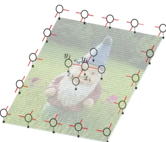
Basic CRFs utilize unary and pairwise potentials on local neighborhoods and it is usually first-order Markov (Fiqure 2.5, Section 2.3.1). Let node vi is in the position of
(k, l) of the graph and |N(i)| = 4 is the number of neighbors. Adjacency CRF can be formulated based on the clique structures that are single and pairwise cliques
C =nCp(i) on i=1∪cs(i) (2.18) Cp(i) = n (ik,l, jk,l−1),(ik,l, jk,l+1),(ik,l, jk−1,l),(ik,l, jk+1,l) o (2.19)
where Cp(i) is the set of pairwise cliques corresponding to node vi, and cs(i) expresses
the single clique. The ability of the adjacency CRF is limited to model long-range inter-node connections and, therefore, generally leads to excessive smoothing of object boundaries. According to Gibbs distributions [45] energy is distributed in the random field until it reaches an equilibrium state. Based on the definition of energy in local random fields, the energy transformation would stop when close nodes have the same state value. In this situation there is no extra energy in one node that can be transformed to its neighbors. It means that close nodes have approximately the same label, which makes
Figure 2.5: Adjacency CRF graphical model; each nodeiis connected to its local neighbors corresponding to the first-order Markov.
the boundaries smoother than desire. This is like transforming heat energy through a metal. Heat propagates through the metal until the whole surface of metal reach to a same temperature. But in the long-range connections the definition of energy can be changed such that, a same label is assigned to the random variables with the same characteristics. In addition to color similarity, the spatial information are incorporated in modeling. In these models the boundaries are preserved better in optimization step.
However fully connected random fields and global connectivity can model different relations among data, modeling of long-range or fully connected graph is not tractable. The computational complexity of long-range connections is the most challenging part of this problem.
In order to improve modeling accuracy and providing the longer connections range, researchers have expanded the basic CRF framework [65, 96] to incorporate hierarchical connectivity and higher-order potentials defined on image regions which will be discussed in section 2.4.2.
2.4.1
Local Random Fields
2D CRFs are useful tools in image processing applications [65,96] due to the image struc-ture. Pixels are related to their neighbors based on the color intensities and statistical features. The color intensity changes smoothly in natural images except at image bound-aries; therefore Gibbs distributions and Markov random fields are appropriate approaches to model image processing and computer vision problems.
Conventional approaches [65, 174] utilized local neighborhood relations in statistical modeling such as CRFs, since the computational complexity increases by increasing the number of connections. In those studies each pixel is represented by a random variable and each random variable is related to others based on the first-order Markov.
The main role of CRFs in an image modeling problem is to incorporate contextual information and spatial relations among variables. Kumar and Hebert [94] proposed a dis-criminative framework based on the CRF to classify the man–made structure from natural scenes. A logistic classifier was applied as the associative potential while a simple Ising model was incorporated to extract interaction relations and to penalize every dissimilar pair of labels by a cost.
Shotton et al. [150] proposed the textonboost method to do object segmentation and object classification simultaneously. The CRF is utilized to capture the spatial interactions among neighbor pixels and also improves the segmentation of specific object instances. To overcome the ambiguities of local appearance of an image patch, they incorporated longer range information such as the spatial layout of an object and also contextual information from the surrounding image by 4-connected grid structure of the CRF. The use of CRF allows them to incorporate texture, layout, color, location, and edge features in a single unified model. Unary potential functions are provided by use of an adapted Joint Boost algorithm [163] which is a type of Adaboost classifier.
Modeling based on 4–connected CRFs imposes some issues in modeling accuracy since the spatial relations are defined at pixel levels and those relations are extracted only based on four neighboring pixels. On the other hand, incorporating larger connections has a
big impact on computational complexity [122]. Due to this fact, some studies have been proposed to incorporate super-pixel [43, 133] instead of pixels as random variables in the random field. In those approaches, a group of close pixels having the same color or statistics are obtained as one node in the random field instead of each pixel.
Fulkerson et al. [43] addressed the image class segmentation and localization by for-mulating the CRF on super-pixels. They obtained super-pixels from a conservative over-segmentation method. The local redundancies of data are captured by aggregating pixels into super-pixels and also it allows the model to measure feature statistics. A bag-of-features classifier was constructed by use of image descriptors such as SIFT. The classifier merges pixels to a region based on extracted features. Since the selected segmentation algorithm is an over-segmented type, boundaries are preserved in the output image. The CRF was utilized to reduce misclassifications that occur near objects’ boundaries. The unary potentials are defined directly by the probability provided by the SVM classifier while, the interaction potentials are a combination of dissimilarity distance on color of super-pixels.
The modeling accuracy of the super-pixel methods is dependent on the accuracy of over-segmentation algorithm. However, there are some other studies which tried to capture both local and global relationships and address this issue [65, 96]. Hierarchical algorithm is a common approach involving global features as well as local features in modeling. The next section will analyze these methods in more details.
2.4.2
Hierarchical Random Fields
Common CRF approaches are based on the quantization of an image space-pixel [96]. The simplest ones utilize each pixel as a random variable in the random field while more complex methods use segments or a group of segments [130]. The goal of segment based representation of pixels as one random variable is to capture global information in order to improve the classification, localization or segmentation accuracy. However segment based (superpixel) approach relaxes the computational complexity, the final accuracy relies upon the initial quantization (superpixel or initial segmentation) over the image space.
Hierarchical approaches are a way that can compensate the effect of initial quantiza-tion [96]. Thanks to the structure of random field modeling, different relations can be incorporated in an unified model. In other words, the local and global interactions can be involved in modeling, simultaneously. Hierarchical models allow the integration of features computed at different levels of the quantization hierarchy.
Hierarchical or multi-scale approaches have been utilized for different applications. Fieguth [38] proposed a multi-scale framework to do the posterior sampling when there exist sparse measurements. The proposed model takes advantage of multi-scale proper-ties to relax the computational complexity of computing the covariance matrix. He also used a hierarchical approach to model the characteristic of a porous media [39] locally and non-locally to sample a new image.
Besides the multi-scale methods proposed in the context of Markov random fields, hierarchical methods have been utilized within the context of conditional random field frameworks as well. The unary and pairwise potentials are computed in different layers. Each layer is constructed based on a quantization level on observations. The CRF plays the role of an unification procedure to combine all potential functions. The final step is the same as common CRFs which is to minimize the energy to find the best state configuration.
He et al. [65] utilized local and global features in a unified hierarchical CRF model to label different regions in an image. Local features are the result of statistical classifiers, such as a neural network. The image is divided into non-overlapped patches to extract the global features. All features are associated with a learned weight in the training step which determines the impact of that feature on the classification and the decision. Inference and finding the optimal label configuration has been done in the lower level (fine level) in order to minimize the proposed energy function.
Ladick´y et al. [96] applied a hierarchical CRF on object class image segmentation. Most of the hierarchical approaches follow the same procedure to define hierarchical levels. The main difference between [65] and [96] is that [96] incorporated additional term in the energy function that represents the label consistency between different layers. Also the unary features were provided with the same method as [150].
Due the weakness of local CRFs, studies have intended to incorporate more global interactions in modeling. It was mentioned that decision just by local features leads to mis-classification [43] in some problems. Classification of “sky” and “water” in an image is a good example for this situation. These two type of objects have the same characteristics locally while they can be distinct by use of global characteristics. Due to this fact, a wide variaty of research [89,169,185] have been conducted to utilize more interactions in modeling and the goal is to take the advantage of all interactions. The ultimate goal is to define a fully connected interactions to acquire an accurate model.
The main challenge of utilizing long-range interactions in random fields is the com-putational complexity since the model complexity increases exponentially by increasing the number of connections in the modeling procedure. To make more intuition about the computational complexity of those models and know how they work, the following sec-tion explains fully connected random fields generally and reviews some efficient proposed approaches to tackle this problem.
2.4.3
Fully Connected Random Fields
The general framework of CRFs is identical for different sizes of connectivities and usually the only difference from a local CRF is the design of interactions among random variables in the field, therefore the formulation of a fully connected CRF (2.20) is the same as adjacency CRFs (2.16)
P(Y|X) = 1 Z(X)exp
−ψ(Y|X) (2.20)
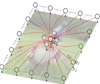
where Z(·) is the partition function and ψ(·) is the combination of unary and pairwise potential functions. The main differences of a fully connected CRF and an adjacency one as shown in Figure 2.6 are the neighborhood size, the number of cliques and their structures. Since the graph is fully connected, each node is in the neighborhood set of all other nodes in the graph,
Figure 2.6: Fully connected conditional random fields; each node is connected to all other nodes in the random field. The connectivities of nodeiare only shown for the visualization purposes. Compared to Figure 2.5 the interested node can be connected to all other nodes in the random fields.
where |N(i)| = n −1. Based on the neighborhood size and the clique structure [160], the number of possible cliques are varied. Different clique structures can be utilized in fully connected modeling but using only the pairwise clique structures is the most common approach [89, 185]. The main reason is that the number of cliques increases the computa-tional complexity of the model in addition to the number of connectivities. Here, without loss of generality the specified clique structure C is assumed to be pairwise clique
C=nCp(i) on i=1 (2.22) Cp(i) = n (i, j)|j ∈N(i)o (2.23)
The inverse of the covariance matrix among random variables (i.e., with computational complexity O(N3) [134]) must be evaluated to find the solution and, therefore, the com-putational complexity of exact inference on a fully connected graph isO(N3).
Due to the high computational complexity of the exact inference, approximation meth-ods have been proposed to tackle this problem [84, 176]. Mean field inference [84] is one
of the tractable frameworks performing a message passing algorithm by approximating each marginal probability. The message passing procedure updates each approximated marginal distribution until convergence. The computational complexity of single iteration of updating the marginal distribution for one random variable isO(N) and the complexity of updating all marginals isO(N2).
The recent method proposed by Kr¨ahenb¨uhl and Koltun [89] reduces the computational complexity of the inference from quadratic to linear by extending the mean field approx-imation. Their inference is highly efficient since a linear combination of Gaussian kernels in an arbitrary feature space is defined as pairwise feature function.
2.5
Efficient Inference Approach
Incorporating long range connectivities is a challenging part of random field modeling. The main advantage of random fields in modeling problems such as image segmentation and im-age classification is that it facilitates the use of spatial information in the model. Although utilizing long range connectivities benefits the model, increasing the size of interactions and spatial relations in the model have a significant impact on computational complexity of the inference step. There are some approximation techniques [84] to relax the compu-tational complexity but they are not helpful when the size of image or observation is very large. There are several methods [89, 186] reformulated the inference problem as filtering and solved the inference step by fast convolutions. Those algorithms are mainly divided into two folds based on the convolution implementation to compute the interactions. The next sections explain those methods in more detail.
2.5.1
Permutohedral Lattice Based Method
Kr¨ahenb¨uhl and Koltun [89] proposed a tractable inference procedure by incorporating specific potential functions. They modeled the multi-class image segmentation by a fully connected CRF where the edge potentials were obtained using Gaussian kernels. By use
of these new feature functions, they reformulated the inference procedure as a filtering problem via a mean-field approximation.
The exact distribution of P(Y|X) is approximated by Q(Y|X). The mean field [84] approximation computes the distribution Q(Y|X) among all distributions Q minimizing the KL-divergence ofQ and P,D(Q||P):
D(Q||P) =X i Qiln Qi Pi . (2.24)
In other words, the product of independent marginals Q(yi|X) over each variable is
computed as an approximation ofP(Y|X) via KL-divergence. However mean field approx-imation relaxes the computational complexity of the inference toO(N2), the computation is not tractable yet when working with large data (e.g., high resolution images). To ad-dress the computational complexity of the fully connected random field, the proposed method [89] utilized a bilateral filtering and a Gaussian smoothness kernel as pairwise fea-ture functions to be able to model the random field in a Permutohedral lattice which can compute the convolution in linear time complexity.
The utilized feature function k(·) is the combination of two contrast-sensitive kernel filters. The first kernel in (2.25) is a bilateral filter which is a nonlinear filter smoothing while preserves strong edges [121] and the second one is a smoothness kernel to remove small isolated regions:
k(i, j) = ω(1)exp− kui−ujk 2θ2 α − kxi −xjk 2θ2 β +ω(2)expkui−ujk 2θ2 γ (2.25)
whereuiandujare the coordinates of nodeiandj in the image;xiandxj are corresponding
features for each node according to the observation. ω(1) and ω(2) are the weights of each feature function determined by cross validation. Since they used Gaussian kernels as pairwise feature functions, the message passing procedure can be seen as a filtering problem. Thanks to a novel data structure (Permutohedral lattice) where reduces the computational complexity of convolution to linear [1] the convolution can be implemented efficiently.
The feature space is represented with simplices arranged alongd+ 1 axes wheredis the feature space dimension. The procedure is divided into four stages: generating position vectors, splatting, blurring, and slicing. The position of each sample must be generated and embedded in the high-dimensional space d+ 1. After that we must identify its enclosing simplex and compute barycentric weights so-called splatting. The third stage is to perform a regular Gaussian blur within that subspace. To do that, splatted data are convolved by the kernel [1 2 1] along each lattice direction. Slicing is identical to splatting, except that it uses the barycentric weights to gather from the lattice points instead of scattering to them.
The proposed method was examined by a multi-label image segmentation problem. The actual computational complexity of the proposed method is O(dN) where d is the dimension of feature space and N is the number of nodes in the random field.
2.5.2
FFT Based Method
Zhang and Chen [185] proposed an alternative method to address the computational com-plexity of the fully connected CRF. Their approach is similar to [89] in the context of filtering. The proposed method modifies the inference of the fully connected CRF to a filtering problem and provides an efficient procedure by doing convolution.
The pairwise feature functions are divided into color contrast and spatial relation:
ψij(yi, yj) =φi,j(ui, uj)ϕi,j(yi, yj, xi, xj) (2.26)
whereφi,j(ui, uj) is the spatial relation of nodeiandj andϕi,j(yi, yj, xi, xj) is color contrast.
The color contrast term encourages a same label when the colors of nodes i and j (xi
and xj) are similar, and different labels otherwise. The spatial relation represents the
categorie


![Table 3.1: Quantitative results (F 1 -score) based on the EnglishHnd dataset [30]. The proposed framework is examined by two noise types with two different levels](https://thumb-us.123doks.com/thumbv2/123dok_us/641713.2577346/77.918.250.685.331.492/quantitative-results-englishhnd-dataset-proposed-framework-examined-different.webp)
![Figure 5.1: Examples images of the Weizmann dataset [148]. This dataset contains images with single and two objects.](https://thumb-us.123doks.com/thumbv2/123dok_us/641713.2577346/97.918.144.813.146.306/figure-examples-images-weizmann-dataset-dataset-contains-objects.webp)