Available at http://www.joics.com
Software Defect Prediction Based on Classifiers Ensemble
Tao WANG
∗
,
Weihua LI, Haobin SHI, Zun LIU
School of Computer, Northwestern Polytechnical University, Xi’an 710072, China
Abstract
Software defect prediction using classification algorithms was advocated by many researchers. However, several new literatures show the performance bottleneck by applying a single classifier recent years. On the other hand, classifiers ensemble can effectively improve classification performance than a single classifier. Motivated by above two reasons which indicate that defect prediction using classifiers ensemble methods have not fully be exploited, we conduct a comparative study of various ensemble methods with perspective of taxonomy. These methods included Bagging, Boosting, Random trees, Random forest, Random subspace, Stacking, and Voting. We also compared these ensemble methods to a single classifier Naïve Bayes. A series of benchmarking experiments on public-domain datasets MDP show that applying classifiers ensemble methods to predict defect could achieve better performance than using a single classifier. Specially, in all seven ensemble methods evolved by our experiments, Voting and Random forest had obvious performance superiority than others, and Stacking also had better generalization ability.
Keywords: Software Defect Prediction; Classifiers Ensemble; Ensemble Methodology
1
Introduction
With software systems are getting more and more complex, the probability of these software systems have defective modules is getting higher. Meanwhile, software quality assurance is a resource and time-consuming task, budget does not allow for complete testing of an entire system. Therefore, identifying which software modules are more likely to be defective can help us allocate limited time and resources effectively. Given recent research in artificial intelligence, data miners, such as Naïve Bayes, ANN, SVM, Decision tree, logistic regression, and association rules etc., are often used to automatically learn predictors for software quality which can identify defective software modules based on software metrics. It has been observed that the majority of a software system’s faults are contained in a small number of modules [1, 2], so the identification of defect prediction can help us allocate test time and resources to a small number of modules that seems defect-prone, although an ideal defect predictor would not be able to identify every defective module.
∗Corresponding author.
Email address: [email protected](Tao WANG).
1548–7741/Copyright© 2011 Binary Information Press
Classification is a kind of most popular approach for software defect prediction [3-6]. Clas-sifiers categorize modules which represented by a set of software complexity metrics or code attributes/features into defect-prone and non-defect-prone by means of a classification model de-rived from data of previous development projects [7]. The well-known software complexity metrics include code size [8], Halstead’s complexity [9] and McCabe’s cyclomatic complexity [10]. Many recent researchers reported the advantages of classification models used to predict defects, such as Tim Menzies et al. [14], E. J. Weyuker et al. [11, 12], Qinbao Song et al. [13], and someone others [15-19].
Meanwhile, the "ceiling effect" of predictors was been found by several researches [20-23]. These results show that better data mining techniques may be not leading to better defect predictors. It seemed that software metrics-based defect prediction reached its performance bottleneck. Con-sequently, some researches tried to break this kind of "ceiling effect". Tim Menzies et al. tried to break the performance ceiling by improving the information content of the training data rather than applying better data mining technics [20]. In another paper of Tim Menzies, They thought that learners must be chosen and customized to the goal at hand and proposed a meta-learner framework WHICH that can tune a learner to specific local business goals rather than the in-discriminate use of learners[21]. Hongyu Zhang et al. thought better defect predictors can be trained from the defect dense components by focusing on the defect-rich portions of the training sets [22]. Yue Jiang et al. hypothesized that future research into defect prediction should change its focus from designing better modeling algorithms towards improving the information content of the training data. They also found that models that utilize a combination of design and code level metrics outperform models which use either one or the other metric set [23]. Yi Liu et al. pre-sented a novel search-based approach to software quality modeling with multiple software project repositories which includes three strategies for modeling with multiple software projects: Base-line Classifier, Validation Classifier, and Validation-and-Voting Classifier [24]. These researches all got various positive conclusions for break the "ceiling effect" by means of different methods.
There are many theoretical and empirical evidences which demonstrate ensemble methodology combine the predictions of multiple classifiers to lead decision-making more accuracy [25-30, 46]. Nevertheless, few researches reported defect prediction model based on ensemble of classifiers. A.Tosun et al. proposed an ensemble model which combines three different algorithms include Naïve Bayes, Artificial Neural Network and Voting Feature Intervals, and considerably improved the defect detection capability compared to Naïve Bayes algorithm[31], but A.Tosun’s works only focus on one ensemble method and few NASA MDP[41] datasets. Jun Zheng analyzed three cost-sensitive boosting algorithms to boost neural networks for software defect prediction [32], but his work focused on boost which is only one method of classifiers ensemble.
We believe that method by using classifiers ensemble to predict software defect has not been fully explored so far in this type of research, so this paper focuses on two questions: (a) how to construct classifiers ensemble? And (b) which popular classifiers ensemble method looks like more effective in defect prediction? In section 2 we will review 7 different popular classifiers ensemble methods from the perspective of taxonomy for characterizing ensemble methods include Bagging, Boosting, Random Forest, Random Tree, Random Subspace, Stacking, and Voting. In section 3 we will implement several experiments for evaluating performance of these methods and comparing them to single classifier. The conclusions are given in section 4.
2
Classifiers Ensemble Based Defect Prediction Models
Ensemble methodology imitates human second nature to seek several opinions before making any crucial decision [27]. Classifiers ensemble, which build a classification model by integrating multiple classifiers, can be used to improve defect prediction performance. The main idea of an ensemble methodology is to combine a set of learning models whose decisions are combined to improve the performance of the overall system. Indeed, ensemble methods can effectively make use of diversity of various types of classifiers to reduce the variance without increasing the bias [26].
We first made following assumptions. For the classification issue to predict defect, the object module m is represented by a set of code attributes, which is m : {a1, a2,· · · , an}. Classifier’s
task is to make decision for whetherm belongs tocd or cnd, where cd is defective class label and
cnd is non-defective class label.
Bagging is Bootstrap AGGregatING [33]. The main idea of Bagging is constructing each member of the ensemble from a different training dataset, and the predictions combined by either uniform averaging or voting over class labels. A bootstrap samples N items uniformly at random with replacement. That means each classifier is trained on a sample of examples taken with a replacement from the training set, and each sample size is equal to the size of the original training set. Therefore, Bagging produces a combined model that often performs better than the single model built from the original single training set.
Algorithm 1 Bagging
Input: the number of ensemble members M
Input: Training set S={(m1, c1),(m2, c2),· · · ,(mN, cN);c1, c2,· · · , cN ∈ {cd, cnd}} Input: Testing setT
Training phase:
for i= 1 to M do
Draw (with replacement) a bootstrap sample set Si (N examples) of the data from S
Train a classifier Ci from Si and add it to the ensemble
end for
Testing phase:
for each t inT do Try all classifiers Ci
Predict the class that receives the highest number of votes end for
Boosting is another popular ensemble method, and Adaboost[34] is the most well-known of the Boosting family of algorithms which trains models sequentially, with a new model trained at each round. Adaboost constructs an ensemble by performing multiple iterations, each time using different example weights. The weight of incorrectly classified examples will be increased, so this ensures misclassification errors for these examples count more heavily in the next iterations. This procedure provides a series of classifiers that complement one another, and the classifiers are combined by voting.
An approach called randomized C4.5 was proposed by Dietterich [35] which has a more popular name "Random Tree". The main idea is randomizing the internal decisions of the learning algorithm. Specifically, it implemented a modified version of the C4.5 learning algorithm in
Algorithm 2 Adaboost
Input: the number of ensemble members M
Input: Training set S ={(m1, c1),(m2, c2),· · · ,(mN, cN);c1, c2,· · · , cN ∈ {cd, cnd}} Initialize: each training example weight wi = 1/N (i = 1· · ·N)
Training phase:
for x= 1 toM do
Tran a classifierCx using the current example weights
compute a weighted error estimate: errx =
∑
(wi of all incorrectly classified mi)/
∑N i=1wi
compute a classifier weight: αx = log((1−errx)/errx)/2
for all correctly classified examples mi :wi ←wie−αx
for all incorrectly classified examplesmi :wi ←wieαx
normalize the weights wi so that they sum to 1
end for
Testing phase:
for each t in T do
Try all classifiers Cx
Predict the class that receives the highest sum of weights αx
end for
which the decision about which split to introduce at each internal node of the tree is randomized. At each node in the decision tree the 20 best tests are determined and the actual test used is randomly chosen from among them. With continuous attributes, it is possible that multiple tests from the same attribute will be in the top 20.
Random Forest [36] approaches to creating an ensemble also utilize a random choice of attributes in the construction of each CART decision tree. The individual trees are constructed using a simple algorithm. The decision tree is not pruned and at each node, rather than choosing the best split among all attributes, the inducer randomly samples N (where N is an input parameter) of the attributes and choose the best split from among those variables. The classification of an unlabeled example is performed using majority vote [27]. The important advantages of the Random Forest method are fast and its ability to handle a very large number of input attributes. Unlikely Random Forest, Random Subspace method creates a decision forest utilizes the random selection of attributes in creating each decision tree [37]. A subset of attributes is uniformly and randomly selected and assigned to an arbitrary learning algorithm. This way, Random Subspace increases the diversity between members of the ensemble. Ho’s empirical studies had suggested good results can be obtained with a uniform and random choose 50% of the attributes to create each decision tree in an ensemble. Random Subspaces was better for data sets with a large number of attributes [37].
Stacking is another ensemble learning technique [38]. In Stacking scheme, there are two level models which are set of base models are called level-0, and the meta-model level-1. The level-0 models are constructed from bootstrap samples of a dataset, and then their outputs on a hold-out dataset are used as input to a level-1model. The task of the level-1 model is to combine the set of outputs so as to correctly classify the target, thereby correcting any mistakes made by the level-0 models.
Voting is a combining strategy of classifiers [39, 40]. Majority Voting and Weighted Majority Voting are more popular methods of Voting. In Majority Voting, each ensemble member votes
for one of the classes. The ensemble predicts the class with the highest number of vote. Weight-ed Majority Voting makes a weightWeight-ed sum of the votes of the ensemble members, and weights typically depend on the classifiers confidence in its prediction or error estimates of the classifier. Kuncheva [39] proposed that classifiers ensemble method can be grouped by the ways of con-struction. There are "Combination level" which defines different ways of combining the classifier decisions, "Classifier level" that indicates which base classifiers are used to constitute the ensem-ble, "Attributes level" in which different attribute subsets can be used for the classifiers, and "Data level" that indicates which dataset is used to train each base classifier. Based on above taxonomy, Bagging and Boosting belong to "Data level", Random tree and Random Subspace belong to "Attributes level", Stacking belongs to "Classifier level", and Voting belongs to "Com-bination level". The exception is Random Forest which commonly is regarded as a hybrid of the Bagging algorithm and the Random Subspace algorithm.
3
Experiments and Results
3.1
Datasets and preprocess
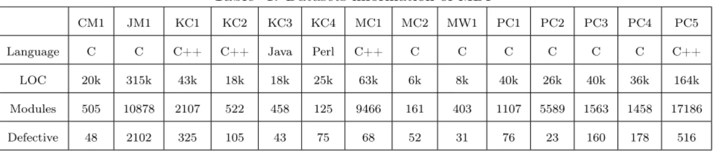
The datasets of experiments used in this paper are NASA IV&V Facility Metrics Data Program (MDP datasets) [41]. As shown by Table 1, MDP datasets involve 14 different datasets collected from real software projects of NASA. Each dataset have many software modules coded by several different programming language including C, C++, Java, and Perl. These datasets have various scales from 125/6k to 186/315k (the numbers of module/the lines of code), and various types of code metrics including code size, Halstead’s complexity and McCabe’s cyclomatic complexity etc. MDP is a public-domain data program which can be used by any researchers and is dataset basis of PROMISE research community [42]. Adapting public-domain datasets in experiment is a benchmarking procedure of defect prediction research which can make different researchers compare their techniques convenience [7, 14]. Our experiments were defined and motivated by such a baseline.
For preparation of our experiments, we performed the following two data preprocessing steps: 1. Replacing missing attribute values. We used the unsupervised filter named ReplaceMissing-Values in Weka [44] to replace all missing attribute values in each data set. ReplaceMissingValues
replaces all missing values with the modes (where attribute value is nominal) and means (where attribute value is numeric) from the training data. In MDP, the attributes values of datasets are all numeric, soReplaceMissingValues replaces all missing values with the means.
2. Discretizing attribute values. Numeric attributes were discretized by the filter of Discretize
in Weka using unsupervised 10-bin discretization.
3.2
Accuracy indicators
We adapted two accuracy indicators in our experiments to evaluate and compare the aforemen-tioned ensemble algorithms, which are classificationaccuracy (AC) and area under curve (AUC) [43]. With a binary classification confusion matrix, we called test example true positive (TP) which is be predicted to positive and is actual positive,false positive (FP) which is be predicted to positive but is actual not, true negative (TN) which is be predicted to negative and is actual
Table 1: Datasets information of MDP
CM1 JM1 KC1 KC2 KC3 KC4 MC1 MC2 MW1 PC1 PC2 PC3 PC4 PC5
Language C C C++ C++ Java Perl C++ C C C C C C C++
LOC 20k 315k 43k 18k 18k 25k 63k 6k 8k 40k 26k 40k 36k 164k
Modules 505 10878 2107 522 458 125 9466 161 403 1107 5589 1563 1458 17186
Defective 48 2102 325 105 43 75 68 52 31 76 23 160 178 516
negative, false negative (FP) which is be predicted to negative but is actual not. So we had AC= (TP+TN)/ (TP+FP+TN+FN). AUC is area under ROC curve. That is also the integral of ROC curve with false positive rate as x axis and true positive rate as y axis. If ROC curve is more close to top-left of coordinate, the corresponding classifier must have better generalization ability so that the corresponding AUC will be lager. Therefore, AUC can quantitatively indicate the generalization ability of corresponding classifier.
In accordance with benchmarking procedure proposed by Stefan Lessmann [7], we also per-formed the statistical hypothesis testingPaired Two-tailed T-test for all algorithms in experiments which can reveal whether there is the significance performance difference between algorithms in statistical. Specifically, Paired Two-tailed T-test is to statistical hypothesis test the mean of two related samples to infer whether there is the statistical significance difference between two means.
3.3
Experiments procedure
For evaluating and comparing performance in software defect prediction of various ensemble methods discussed above and a single classifier, we employed the Weka tool which implements all algorithms we need in experiments. These algorithm packets are Bagging, AdaBoostM1 (which is most popular version of boosting), NaïveBayes (which is a most popular single classifier sim-ple and effective), RandomForest, RandomTree, RandomSubspace, Stacking, and Vote. Bagging, AdaBoostM1 and RandomSubspace are all meta-learner, so we assigned the NaïveBayes to base classifier of these algorithms. We selected four base classifiers for Vote evolving NaïveBayes, Logistic, libSVM, and J48, because these are all most popular algorithms in software defect pre-diction research community. ThecombinationRule of Vote is average of probabilities. We also let the level-1 classifiers ofStacking be these four algorithms, and the level-0 classifier beNaïveBayes.
In all experiments, we performed10-fold cross validation. That means we will got 100 accuracy values/ACU values for each algorithm on each dataset, this way, the mean of these 100 values is the average accuracy/average AUC for this algorithm on this dataset.
Experiments procedure:
Input: the MDP datasets: D ={CM1, JM1, KC1, KC2, KC3, KC4, MC1, MC2, MW1, PC1, PC2, PC3, PC4, PC5}
Input: all algorithms: A ={Bagging, AdaBoostingM1, NaïveBayes,RandomForest, Ran-domTree, RandomSubspace, Stacking, Vote}
Dataset preprocess:
a. Replacing missing attribute values. Apply ReplaceMissingValues of Weka to D. b. Discretizing attribute values. ApplyDiscretize of Weka toD.
10-fold cross validation:
for each dataset in D do
for each algorithm in A do
Perform 10-fold cross validation. end for
PerformPaired Two-tailed T-test.
end for
Output:
a. Accuracy and standard deviation of 8 classifiers on 14 datasets. b. AUC and standard deviation of 8 classifiers on 14 datasets. c. The results of Paired Two-tailed T-test.
3.4
Results and discusses
We had got experiment results about accuracy of various algorithms on various datasets as shown by Table 2. We draw the following observations from these experiment results:
• Because we let NaïveBayes be the base classifier for Bagging and AdaBoostM1, we first focused on performance difference between these three algorithms. Nevertheless, we were surprised and found that Bagging and AdaBoostM1 hardly can improve the classification accuracy relative to NaïveBayes. On 11 of all datasets besides KC4, PC3, and PC5, the
Bagging with NaïveBayes for base classifier even got lower accuracy by NaïveBayes. The AdaBoostM1 also got similar results on 9 of all datasets besides MC1, MW1, PC1, PC2, and PC3. Although total mean of accuracy of Bagging or AdaBoostM1 are all higher than
NaïveBayes, but the improvements even not achieve 0.5 percent.
• Same as above two algorithms, RandomSubSpace also has NaïveBayes for base classifier. However, RandomSubSpace improved the classification accuracy on 12 of all datasets only besides MC2 and JM1, and improved the total mean of accuracy 1.12 percent byNaïveBayes.
• Vote got best classification performance on 7 of 14 datasets, and RandomForest got best classification performance on 4 datasets. So only on 3 datasets, there were best classification performances got by other algorithms besides above two.
• Focusing on the total mean of every datasets, we found the performance of RandomForest, RandomTree, Stacking, andVotewas obviously better thanNaïveBayes and other ensemble methods. Vote got the highest mean of accuracy 88.48% followed by 87.90% of Random-Forest. These two algorithms obviously outperformed than others.
Table 2: AC (%) and standard deviation of various classifiers on 14 datasets
Dataset Bagging AdaBoostM1 NaïveBayes RandomForest RandomTree RandomSubSpace Stacking Vote
CM1 84.15±4.89 84.32±5.69 84.58±4.90 89.11±2.19 85.01±4.28 85.58±4.94 83.49±5.56 89.64±2.30 JM1 80.40±0.91 80.45±0.88 80.45±0.88 79.66±0.98 75.30±1.26 80.41±0.84 79.19±1.11 81.44±0.56 KC1 82.44±2.22 82.50±2.23 82.50±2.23 85.47±1.81 82.85±2.44 82.77±2.06 81.41±2.43 85.62±1.64 KC2 83.53±3.47 83.60±3.41 83.62±3.42 82.62±4.22 79.86±4.86 83.82±3.37 81.52±4.28 82.91±3.38 KC3 84.74±5.06 84.70±4.98 84.78±5.00 89.72±2.40 87.39±4.43 85.41±5.17 85.24±5.35 89.98±3.20 KC4 65.81±11.05 64.48±10.47 64.48±10.47 72.81±11.70 70.14±12.29 64.88±10.92 76.58±10.68 75.38±11.43 MC1 93.73±1.12 93.86±1.38 93.80±1.02 99.51±0.13 99.43±0.21 94.15±0.99 97.20±1.12 99.42±0.13 MC2 73.00±8.51 73.09±9.39 73.62±8.04 70.39±10.10 64.05±12.19 73.31±8.03 72.12±9.44 72.57±7.14 MW1 83.12±5.36 87.43±4.73 83.35±5.25 90.58±2.75 87.65±4.48 84.54±5.13 88.63±4.03 91.67±3.07 PC1 89.04±2.59 89.90±2.70 89.12±2.59 93.63±1.53 91.64±2.11 89.49±2.32 88.64±2.95 93.73±1.45 PC2 96.73±1.03 97.13±0.94 97.11±0.92 99.56±0.10 99.29±0.23 97.44±0.80 97.0±00.88 99.53±0.13 PC3 51.00±11.43 51.45±13.84 48.30±10.00 89.83±1.35 86.01±2.59 59.22±10.94 87.01±2.68 89.12±1.77 PC4 86.99±2.86 86.78±3.27 87.11±2.57 90.13±2.05 87.74±2.83 87.30±2.48 87.67±2.66 90.28±1.75 PC5 96.51±0.36 96.44±0.38 96.44±0.38 97.54±0.26 97.08±0.37 96.58±0.39 96.01±0.48 97.46±0.23 MEAN 82.23±2.92 82.58±3.16 82.09±2.69 87.90±1.54 85.25±2.47 83.21±2.74 85.84±3.12 88.48±2.01
• We concluded that some classifier ensembles methods could significantly improve the clas-sification performance than single classifier.
We performedPaired Two-tailed T-test for 100 accuracy values got by every algorithm pair on each dataset as Table 3 shown. We set significance level to be 0.05, and an entry w/t/l of Table 3 means that in statistical the approach at the corresponding row wins in w datasets, ties in t
datasets, and loses in l datasets, compared to the approach at the corresponding column. We draw some observations from test results:
• The score of Vote vs. NaïveBayes was 12 wins, 2 ties, and 0 losses. Vote overwhelmingly defeated NaïveBayes in statistical sense. The score of Vote vs. RandomForest is 1 wins, 12 ties, and 1 loss, so these two algorithms had no significance difference. However, Vote
obviously outperformed other ensemble algorithms besidesRandomForest. This observation coincided with the conclusion about Vote form Table 2.
• RandomForest also had obvious statistical superiority than other algorithms (including
NaïveBayes) besides Vote on majority part of datasets.
• Bagging vs. NaïveBayes had no wins and even loss on one dataset. Similarly, AdaBoostM1
vs. NaïveBayes only had 1 win and 13 ties score.
Furthermore, we had a hypothesis for t-test experiments which supposed two group samples satisfy the normal distribution. This hypothesis may be not suitable for our experiment data which not sure satisfy the normal distribution, and may have some outliers. So we had not
Table 3: The compared results of paired two-tailed t-test on AC with the 0.05 significance level
Bagging AdaBoostM1 NaïveBayes RandomForest RandomTree RandomSubSpace Stacking AdaBoostM1 2/12/0 NaïveBayes 1/13/0 0/13/1 RandomForest 10/3/1 9/4/1 10/3/1 RandomTree 6/6/2 4/7/3 6/6/2 0/6/8 RandomSubSpace 4/10/0 2/12/0 3/11/0 1/3/10 2/7/5 Stacking 4/7/3 3/8/3 4/7/3 0/5/9 1/9/4 4/6/4 Vote 12/2/0 12/2/0 12/2/0 1/12/1 9/5/0 12/2/0 11/3/0
learned about entire information of experiments data. We employed the boxplot to visually show classification accuracy values and outliers of various algorithms on various datasets. As Figure 1 shown, on 12 of all datasets besides KC2 and MC2, accuracy data ofVotehad obvious distribution superiority than other algorithms. This superiority means that boxplot ofVote was located more higher in coordinate system, and the Interquartile Range (IQR) was more small which indicated that data distribution was more centralized relatively. RandomForest also had this distribution superiority than other algorithms besides Vote on datasets besides JM1, KC2, and MC2. These conclusions aboutVoteandRandomForestwere basically similar to the conclusions draw by Table 2 and Table 3.
Table 4: AUC and standard deviation of various classifiers on 14 datasets
Dataset Bagging AdaBoostM1 NaïveBayes RandomForest RandomTree RandomSubSpace Stacking Vote
CM1 0.77±0.11 0.72±0.10 0.77±0.10 0.72±0.13 0.57±0.10 0.76±0.11 0.79±0.11 0.80±0.11 JM1 0.69±0.02 0.58±0.03 0.69±0.02 0.72±0.02 0.59±0.02 0.69±0.02 0.72±0.02 0.73±0.02 KC1 0.79±0.04 0.79±0.04 0.79±0.04 0.80±0.05 0.62±0.06 0.79±0.03 0.81±0.04 0.81±0.04 KC2 0.85±0.06 0.68±0.06 0.84±0.06 0.80±0.07 0.62±0.11 0.85±0.06 0.84±0.06 0.83±0.06 KC3 0.82±0.08 0.75±0.10 0.83±0.08 0.80±0.11 0.61±0.11 0.82±0.08 0.80±0.11 0.80±0.11 KC4 0.76±0.14 0.71±0.14 0.78±0.13 0.80±0.12 0.70±0.13 0.77±0.13 0.83±0.11 0.83±0.12 MC1 0.92±0.04 0.88±0.05 0.90±0.05 0.88±0.09 0.78±0.10 0.92±0.04 0.92±0.08 0.95±0.04 MC2 0.72±0.13 0.73±0.14 0.72±0.12 0.70±0.15 0.58±0.13 0.72±0.13 0.76±0.14 0.76±0.14 MW1 0.77±0.14 0.75±0.14 0.76±0.14 0.72±0.15 0.58±0.13 0.77±0.14 0.77±0.13 0.76±0.14 PC1 0.76±0.08 0.72±0.07 0.75±0.08 0.81±0.09 0.67±0.08 0.74±0.08 0.82±0.10 0.85±0.07 PC2 0.84±0.14 0.73±0.17 0.82±0.15 0.64±0.15 0.51±0.07 0.87±0.11 0.78±0.20 0.87±0.12 PC3 0.77±0.07 0.76±0.07 0.76±0.07 0.81±0.06 0.64±0.06 0.76±0.07 0.83±0.05 0.82±0.06 PC4 0.84±0.05 0.80±0.05 0.84±0.05 0.92±0.03 0.71±0.07 0.83±0.05 0.93±0.03 0.92±0.03 PC5 0.84±0.03 0.83±0.03 0.83±0.03 0.95±0.02 0.73±0.04 0.94±0.01 0.96±0.01 0.96±0.01 MEAN 0.80±0.08 0.75±0.09 0.79±0.08 0.79±0.09 0.64±0.09 0.80±0.08 0.83±0.09 0.84±0.08
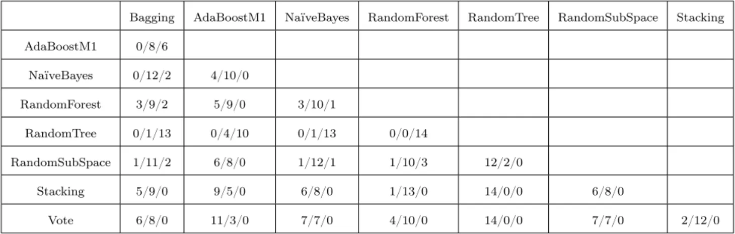
Table 4 shows the detailed AUC values and standard deviation of various algorithms on all datasets. Vote got best AUC of experiments on 9 datasets and the best mean of AUC on all datasets. So Vote presents the best generalization ability with AUC numerical mode. However, it was surprised that RandomForest which was outstanding in classification accuracy and related statistical test had poor AUC values similar to other algorithms besides Vote and Stacking, and only outperformed one algorithm RandomTree. Meanwhile, we found the Stacking got very remarkable performance indicated by AUC value. It got best AUC of experiments of 7 datasets and the top 2 mean of AUC on all datasets second only to Vote. This means that Stacking also has outstanding generalization ability.
Table 5: The compared results of paired two-tailed t-test on AUC with the 0.05 significance level
Bagging AdaBoostM1 NaïveBayes RandomForest RandomTree RandomSubSpace Stacking AdaBoostM1 0/8/6 NaïveBayes 0/12/2 4/10/0 RandomForest 3/9/2 5/9/0 3/10/1 RandomTree 0/1/13 0/4/10 0/1/13 0/0/14 RandomSubSpace 1/11/2 6/8/0 1/12/1 1/10/3 12/2/0 Stacking 5/9/0 9/5/0 6/8/0 1/13/0 14/0/0 6/8/0 Vote 6/8/0 11/3/0 7/7/0 4/10/0 14/0/0 7/7/0 2/12/0
Table 5 shows the compared results ofPaired Two-Tailed T-Test on AUC values. The signifi-cance level of test and the mean of entry are all coincide with Table 3. The scoreboard’s top 3 are
Vote, Stacking, and RandomForest which in statistical sense demonstrated the conclusions draw by Table 4.
4
Conclusions
In this paper, we conduct a comparative study of seven classifiers ensemble methods with context of software defect prediction. These algorithms or methods have different ensemble construction scheme which focus on different "level". Experiment results show us that some of seven algorithms applied to software defect prediction could achieve obvious performance improvement than a single classifier. Various indicators including average classification accuracy, average AUC, and boxplot all provided evidence for Voting which got best performance of all ensemble algorithm and single classifier. Random Forest has second performance only to Voting, but the generalization ability of Random Forest is not better than Stacking. All these proofs let us to advocate the Voting algorithms applied to defect prediction.
In our future works, we plan continue to evaluate various ensemble algorithms by applying different base classifiers which can identify whether our conclusions inflected by base classifiers adopted by our experiments or not.
Acknowledgements
This work is supported by the National High-Tech Research and Development Plan of China under grant No.2006AA01Z406, also supported by the National Natural Science Foundation of China under grant No. 61003129, the Doctorate Foundation of Northwestern Polytechnical University under grant No.CX200815, the Planned Science and Technology Project of ShaanXi Province, China under grant No. 2010JM8039 and the Youth Foundation of ShaanXi Normal University under grant No.200701016.
References
[1] C. Andersson. A Replicated Empirical Study of a Selection Method for Software Reliability Growth Models. Empirical Software Engineering, vol. 12, no. 2, pages 161 – 182, 2007.
[2] N. E. Fenton and N. Ohlsson. Quantitative Analysis of Faults and Failures in a Complex Software System. IEEE Transactions on Software Engineering, vol. 26, no. 8, pages 797 – 814, 2000. [3] T. J. Ostrand, E. J. Weyuker and R. M. Bell. Predicting the location and number of faults in large
software systems. IEEE Transactions on Software Engineering, vol. 31, no. 4, pages 340 – 355, 2005.
[4] N. E. Fenton, P. Krause and M. Neil. Software Measurement: Uncertainty and Causal Modeling. IEEE Software, vol. 10, no. 4, pages 116 – 122, Aug., 2002.
[5] N. Nagappan and T. Ball. Using software dependencies and churn metrics to predict field failures: An empirical case study. In the Proceedings of the First International Symposium on Empirical Software Engineering and Measurement (ESEM’07), pages 364 – 373, 2007.
[6] B. Turhan and A. Bener. A multivariate analysis of static code attributes for defect prediction. In the Proceedings of Seventh International Conference on Quality Software (QSIC’07), pages 231 – 237, 2007.
[7] S. Lessmann, B. Baesens, C. Mues and S. Pietsch. Benchmarking classification models for soft-ware defect prediction: A proposed framework and novel findings. IEEE Transactions on Softsoft-ware Engineering, vol. 34, no. 4, pages 485 – 496, Aug., 2008.
[8] A. G. Koru, K. Emam, D. Zhang, H. Liu, and D. Mathew. Theory of relative defect proneness. Empirical Software Engineering, vol. 13, no. 5, pages 473 – 498, Oct., 2008.
[9] T. McCabe. A complexity measure. IEEE Transactions on Software Engineering, vol. 2, no. 4, pages 308 – 320, Dec. 1976.
[10] M. H. Halstead. Elements of Software Science. Elsevier, North-Holland, 1975.
[11] E. J. Weyuker, T. J. Ostrand, and R. M. Bell. Adapting a Fault Prediction Model to Allow Widespread Usage. In the Proceedings of the 4th International Workshop on Predictive Models in Software Engineering (PROMISE08), Leipzig, Germany, May 12 – 13, 2008.
[12] E. J. Weyuker, T. J. Ostrand, and R. M. Bell. Do too many cooks spoil the broth? Using the number of developers to enhance defect prediction models. Empirical Software Engineering, vol. 13, no. 5, pages 539 – 559, 2008.
[13] Q. Song and M. Shepperd, Software Defect Association Mining and Defect Correction Effort Pre-diction. IEEE Transactions on Software Engineering, vol. 32, no. 2, pages 69 – 82, 2006.
[14] T. Menzies, J. Greenwald, and A. Frank. Data mining static code attributes to learn defect pre-dictors. IEEE Transactions on Software Engineering, vol. 33, no.1, pages 2 – 13, 2007.
[15] N. Nagappan and T. Ball. Using software dependencies and churn metrics to predict field failures: An empirical case study. In the Proceedings of the First International Symposium on Empirical Software Engineering and Measurement (ESEM’07), pages 364 – 373, Washington, DC, USA, 2007. [16] N. F. Schneidewind. Investigation of Logistic Regression as a Discriminant of Software Quality. In the Proceedings of IEEE CS Seventh Int’l Conf. Software Metrics Symp., pages 328 – 337, Apr. 2001.
[17] L. Guo, B. Cukic, and H. Singh. Predicting Fault Prone Modules by the Dempster-Shafer Belief Networks. In the Proceedings of IEEE CS 18th Int’l Conf. Automated Software Eng., pages 249 – 252, Oct. 2003.
[18] T.M. Khoshgoftaar and N. Seliya. Comparative Assessment of Software Quality Classification Tech-niques: An Empirical CaseStudy. Empirical Software Engineering, vol. 9, no. 3, pages 229 – 257, 2004.
[19] N. Gayatri, S. Nickolas, A. Reddy, and R. Chitra. Performance analysis of data mining algorithms for software quality prediction. In the Proceeding of International Conference on Advances in Recent Technologies in Communication and Computing (ARTCom’09), pages 393 – 395, 2009. [20] T. Menzies, B. Turhan, A. Bener, G. Gay, B. Cukic, and Y. Jiang. Implications of Ceiling Effects
in Defect Predictors. In the Proceedings of the 4th International Workshop on Predictive Models in Software Engineering (PROMISE’08), Leipzig, Germany, May 12 – 13, 2008.
[21] T. Menzies, Z. Milton, B. Turhan, B. Cukic, Y. Jiang, and A. Bener. Defect prediction from static code features: current results, limitations, new approaches. Automated Software Engineering, vol. 17, no. 5, pages 375 – 407, May, 2010.
[22] H. ZhangčňA. Nelson and T. Menzies. On the Value of Learning from Defect Dense Components for Software Defect Prediction. In Proceedings of the 6th International Conference on Predictive Models in Software Engineering (PROMISE’10), Sep12 – 13, Timisoara, Romania, 2010.
[23] Y. Jiang, B. Cukic, T. Menzies, and N. Bartlow. Comparing Design and Code Metrics for Software Quality Prediction. In the Proceedings of the 6th International Conference on Predictive Models in Software Engineering (PROMISE’10), Sep12 – 13, Timisoara, Romania, 2010.
[24] Y. Liu, T. M. Khoshgoftaar, and N. Seliya. Evolutionary optimization of software quality modeling with multiple repositories. IEEE Transactions on Software Engineering, vol. 36, no. 6, pages 852 – 864, 2010.
[25] C. D. Stefano, F. Fontanella, G. Folino and A. S. Freca. A Bayesian Approach for combining en-sembles of GP classifiers. In the Proceedings of the 10th International Workshop Multiple Classifier Systems (MCS’2011), Naples, Italy, June 15 – 17, 2011.
[26] D. Windridge. Tomographic Considerations in Ensemble Bias/Variance Decomposition. In the Pro-ceedings of the 9th International Workshop Multiple Classifier Systems (MCS’2010), April 7 – 9, Cairo, Egypt, 2010. Lecture Notes in Computer Science, vol. 5997, pages 43 – 53, Apr. 2010. [27] L. Rokach. Taxonomy for characterizing ensemble methods in classification tasks: A review and
annotated bibliography. Computational Statistics & Data Analysis, vol. 53, no. 12, pages 4046 – 4072, 1 October 2009.
[28] J. J. Rodrĺłguez, L. I. Kuncheva, and C. J. Alonso. Rotation forest: A new classifier ensemble method. IEEE Transactions on Patten Analysis and Machine Intelligence, vol. 28, no. 10, pages 1619 – 1630, Oct. 2006.
[29] R.E. Banfield, L.O. Hall, K.W. Bowyer, and W. P. Kegelmeyer. A Comparison of Decision Tree Ensemble Creation Techniques. IEEE Transactions on Pattern Analysis and Machine Intelligence, vol. 29, no. 1, pages 173 – 180, January 2007.
[30] J. Canul-Reich, L. Shoemaker and L. O. Hall. Ensembles of Fuzzy Classifiers. In the Proceedings of IEEE International Conference on Fuzzy Systems (FUZZ-IEEE’07), Imperial College, London, UK, 23 – 26 July, 2007.
[31] A. Tosun. Ensemble of Software Defect Predictors: A Case Study. In the Proceedings of the 2nd International Symposium on Empirical Software Engineering and Measurement (ESEMąŕ08), Oct 9 – 10, Kaiserslauten, Germany, 2008.
[32] J. Zheng. Cost-sensitive boosting neural networks for software defect prediction. Expert Systems with Applications, vol. 37, no. 6, pages 4537 – 4543, 2010.
[33] L. Breiman. Bagging predictors. Machine Learning, vol. 24, no. 2, pages 123 – 140, 1996.
[34] Y. Freund and R. Schapire. Experiments with a new boosting algorithm. In the Proceedings of International Conference on Machine Learning, 1996.
[35] T. Dietterich. An experimental comparison of three methods for constructing ensembles of decision trees: bagging, boosting, and randomization. Machine Learning, vol. 40, no. 2, pages 139 – 157, 2000.
[36] L. Breiman. Random forests. Machine Learning, vol. 45, no. 1, pages 5 – 32, 2001.
[37] T. K. Ho. The random subspace method for constructing decision forests. IEEE Transactions on Pattern Analysis and Machine Intelligence, vol. 20, no. 8, pages 832 – 844, 1998.
[38] D. H. Wolpert. Stacked Generalization. Neural Networks, vol. 5, no. 2, pages 241 – 259, 1992. [39] L. I. Kuncheva. Combining Pattern Classifiers: Methods and Algorithms. John Wiley and Sons,
Inc. 2004.
[40] J. Kittler, M. Hatef, R. P. W. Duin, and J. Matas. On Combining Classifiers. IEEE Transactions on Pattern Analysis and Machine Intelligence, vol. 20, no. 3, pages 226 – 239, March 1998. [41] M. Chapman, P. Callis, and W. Jackson. Metrics Data Program. NASA IV and V Facility,
http://mdp.ivv.nasa.gov/,2004.
[42] G. Boetticher, T. Menzies and T. Ostrand. PROMISE Repository of empirical software engineer-ing data http://promisedata.org/ repository, West Virginia University, Department of Computer Science, 2007.
[43] F. Provost and T. Fawcett. Robust Classification for Imprecise Environments. Machine Learning, vol. 42, no. 3, pages 203 – 231, 2001.
[44] M. Hall, E. Frank, G. Holmes, B. Pfahringer, and P. Reutemann. the WEKA Data Mining Software: An Update; SIGKDD Explorations, Ian H. Witten, vol. 11, no. 1, pages 10 – 18, 2009.
[45] J. Demˇsar. Statistical Comparisons of Classifiers over Multiple Data Sets, Journal of Machine Learning Research, vol. 7, no. 12, pages 1 – 30, 2006.
[46] Y. ZHU, J. OU, G. CHEN, H. YU. An Approach for Dynamic Weighting Ensemble Classifiers Based on Cross-validation. Journal of Computational Information Systems, Vol. 6, no. 1, pages 297 – 305, 2010.