Shallow cumulus clouds

(1)

Shallow cumulus clouds

A parameter study of the development and stability of cumulus clouds in the Atmospheric Boundary Layer Bachelor Thesis September 2005 Bas Reintjes Supervisor: Drs. T. Heus Dr. H.J.J. Jonker

Department of Multi Scale Physics Delft University of Technology Faculty of Applied Sciences

(2)

1.Introduction

Clouds exist in a variety of formats and types. One classification focuses on the height at which clouds form. There are clouds that form at high altitudes (generally above 6 km) these are known as cirriform clouds. Then there are altoform clouds that form at mid-altitudes (between 2-6 km) and clouds that form at even lower altitudes, the stratus and cumulus type clouds. The focus of this research is on the lowest cloud layer. The clouds that form in the lowest cloud layer form are a part of what is generally referred to as the Atmospheric (or Planetary) Boundary Layer (ABL). This is that part of the atmosphere that is influenced by the earth's surface.

Within the lowest cloud layer a classification of clouds is once more possible. There are clouds that cover almost the entire sky. These clouds are said to have a cloud cover close to unity. As one can imagine (and most likely have observed in their daily lives) there are also clouds with a low cloud cover (between 5 – 20%). These clouds are referred to as shallow cumulus, or fair-weather cumulus as good weather normally accompanies this kind of cloud. The shallow cumuli almost never produce precipitation. The focus of this research is on these clouds.

Shallow cumulus plays an important role in large parts of our atmosphere. Most notably in the (sub)tropics, but also in more moderate climates. Shallow cumulus is, when present, to a great extent responsible for the transport of energy through the boundary layer. When clouds form heat is released (due to the condensation of water droplets) and this in turn changes important characteristics of the ABL. This indicates that shallow cumulus is important in weather forecasting and climate prediction. General Circulation Models (GCM's), which have a domain that cover the whole globe, use parametrizations to incorporate the effects of cumulus clouds. The typical grid scale of a GCM is on the order of 10 – 100 km, whereas a typical cumulus cloud has a maximum size of about 1 km. Due to this fact cumulus clouds cannot be directly implemented in GCM's and therefore parametrizations are needed. There are two ways to study cumulus clouds and test parametrizations. One is through observations in the form of aircraft and radar measurements and weather balloons. The other approach is modeling cloud dynamics using Large Eddy Simulations (LES) or Direct Numerical Simulation (DNS). As DNS is computationally very intensive because all turbulent scales need to be resolved one frequently takes refuge in LES, where only the largest turbulent scales are resolved. To improve on the modeling of cloud dynamics it is important to know under what conditions the shallow cumulus simulations stay stable and link this to observations.

This research aims at looking into the causes and effects of shallow cumulus clouds. So far little is known about how changing large scale forcings and initial profiles influences the stability and mean profiles of shallow cumulus simulations. In most recent articles well known cases are used

(4)

without changing any of the initial values. These cases are e.g. BOMEX and ATEX. BOMEX is the Barbados Oceanographic and Meteorological Experiment (Holland & Rasmusson (1973)), ATEX the Atlantic Trade wind experiment (Augustein et al. (1973)). These experiments were conducted in the early 70's and were extensive studies of trade wind regimes. As these cases are frequently used one can ask the question in how far the models are of use in other situations. So our main goal is to vary a limited number of initial parameters and see how this influences the outcome of the simulations, most notably mean profiles. Furthermore it is interesting to see under which conditions the shallow cumulus stays stable as this might tells us something about underlying processes. Summing up what is being studied are the effects of the initial set up on the LES outcome.

The objective of this study is therefore to try to give guidelines which lead to shallow cumulus. Recently scaling laws (e.g. Stevens (2004), Grant & Lock (2004) ) have been proposed that should lead to stable cumulus. The scaling by Grant & Lock will be critically reviewed and tested in as far possible. The study is rather heuristic in approach as many issues still remain vague. As Siebesma et al. (2003) indicate the use of LES to develop new field campaigns is still in its infancy. In this respect the research tries to give a modest Ansatz to the design of such a campaign. It does so by testing different initial set ups for shallow cumulus. An ultimate goal is of course to deduce boundaries in initial profiles and large scale forcings for shallow cumulus clouds to form, but this is considered beyond the scope (and scale) of this study.

The next chapter gives some necessary theory and develops an understanding of the formation of (shallow cumulus) clouds. Furthermore a short introduction to LES will be given. Chapter three focuses on the methodology we have adopted in conducting the research. Chapter four describes the actual set up of the sensitivity experiments. A conclusion and discussion of the results is given in the final chapter.

(5)

2.Theory

This chapter gives a short overview of the relevant concepts. The first paragraph describes the relevant equations determining the formation of clouds. The next paragraph will focus on the actual formation of cumulus clouds in a more qualitative way. Hereafter we will shortly touch upon the turbulent kinetic energy (TKE) relation as it provides a way of understanding the turbulent flows that take place in the atmospheric boundary layer. We will conclude the chapter with a short introduction to the use of LES.

2.1.Governing equations

In this research extensive use is made of elementary thermodynamics. We will not give a full overview of this subject but instead touch some of the less known concepts. The reader not too familiar with thermodynamics can use any elementary text book on thermodynamics. A good description of the use of thermodynamics in meteorological research can be found in Garratt (1992), Stull (1988) or De Roode (2004).

When considering atmospheric thermodynamics one derives appropriate conserved variables. Consider a volume of air that contains a certain amount of water vapor. The ratio between the water vapour and the total mass of the volume of air is called the water vapor specific humidity and denoted q_v_{. In shallow cumulus clouds there is also an amount of liquid water, denoted as}q_l_{. The}

total specific humidity is now given by

(2.1) where we have omitted the content of water in the ice state as this is negligible in shallow cumulus clouds. Obviously the total specific humidity is a conserved variable as the water can change phase between water vapor and liquid water but cannot disappear. As long as the parcel of air is unsaturated, trivially, qt=qv. Now one can define a temperature scale that corrects the ideal

gas law for the presence of moisture. The ideal gas law is given by

(2.2) where p is the pressure, V is the volume N is the number of molecules k = 1.38x10-23_JK-1_{is the}

Boltzmann constant, n is the number of moles of gas and R= 8.341 J mol-1_K-1_{is the universal gas}

constant. The corrected temperature scale is the so called virtual temperature and is defined as (2.3) where R_d=287.0J kg−1_K−1_{is the specific gas constant for dry air and} _R

v=461.5J kg−

1_K−1_{is the}

gas constant for moist air. Tv is the temperature dry air must have to equal the density of moist air at

the same pressure. As such it is also referred to as the density temperature. The liquid water specific

q_t=q_vq_l Tv=T[1−1− R_d Rv qv−ql] pV=NkT=nRT

(6)

humidity tends to diminish the virtual temperature, so in the absence of liquid water the virtual temperature is always greater than the “normal” temperature.

Another useful temperature scale is the potential temperature. In the atmosphere the pressure decreases with an increase in altitude. As a parcel of air rises this has a direct effect on the temperature of the parcel, because it expands due to the lower environmental pressure at a higher altitude. To correct for these pressure effects the potential temperature is used. This is the temperature an unsaturated parcel of air would have if brought adiabatically from its initial state to a standard pressure, p₀, typically 1000 hPa. It reads as

(2.4) where c_p=1005.7J kg−1_K−1_{is the specific heat capacity of dry air at a constant pressure. Of course}

one can substitute Tv for T to arrive at the virtual potential temperature, v. The virtual potential

temperature can be seen as a measure for the buoyancy of an air parcel, with respect ot its environment. Buoyancy is the important mechanism in the formation of clouds. The buoyancy force is consequently given by

(2.5) where v denotes the slab averaged virtual potential temperature and v , core is the parcels'

virtual potential temperature. When a parcel is warmer than its environment it is positively buoyant. One last temperature scale is worth mentioning as it is a conserved quantity in reversible adiabatic motion (in the absence of precipitation). This is the liquid water potential temperature which is defined as

(2.6) where lv is the latent heat of vaporization and =

p p0

Rd/cp is the Exner function. The approximate form of l omits the Exner function.

Having described the conserved variables we turn ourselves to the equations that describe the ABL. These are the continuity equation (conservation of mass), the momentum equation (Navier-Stokes equations) and the equations for the conservation of thermal energy (thermodynamic equation) and conservation of water vapour (humidity equation). For a thorough description of these equations the book by Tennekes and Lumley (1972) is a classic, Garratt (1992), among others, provides an overview for these equations in the ABL.

=Tp0 p  Rd cp l=− lvql c_p F_b=g v , core−v v

(7)

In the present study we are making use of a filtered form of these equations1_{, whereby use is}

made of the Boussinesq approximation. The Reynolds decomposition for the humidity equation is given by

(2.7) and the thermodynamic equation is given by

(2.8) The S_ are source/sink terms. The 〈⋯〉 denotes an ensemble averaged (mean) quantity, whereas a prime denotes a fluctuating quantity. The ui and xi are the velocity- respectively

position-components in the x,y,z (i,j,k) direction. In the thermodynamic equation the most important source/sink terms are the radiative cooling, the surface fluxes and the molecular diffusion. In the humidity equation the sink term is the molecular diffusion. The momentum equation reads asf

(2.9) where g is the gravitational acceleration, i3 is the Kronecker delta, ijk is the alternating unit

tensor and finally  is the angular velocity of the earth's rotation. The last term in the momentum equation accounts for viscosity effects. To solve the governing equations some sort of closure is needed. The LES-code used in this study (Cuijpers and Duynkerke (1993)) uses a one-and-a-half order closure based on eddy-diffusivities.

2.2.Formation of clouds

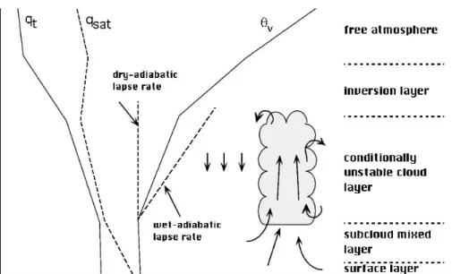
As this research is limited to shallow (fair-weather) cumulus clouds the formation of clouds as discussed here is limited to these type of clouds. The formation of cumulus in the ABL is a process driven by turbulence. The formation of shallow cumulus can be understood by looking at the lapse rate __v. This is the rate at which a given quantity changes with respect to height, in this case virtual potential temperature. For active shallow cumulus to develop it is important that _v is in between the dry-adiabatic lapse rate (which is zero by definition) and the wet-adiabatic lapse rate (which is positive due to the release of latent heat), that is, a so-called conditionally unstable lapse rate. Conditional instability means that the air is stable under the condition that the air is not saturated, and unstable if the air is saturated, as the air is saturated there is latent heat release due to condensation. The situation is summarized in figure 2.1.

When a parcel of air ascends under the influence of the heating of the surface it depends on the 1 This is due to the fact that we are making use of LES.

∂qt ∂t 〈ui〉 ∂ 〈qt〉 ∂xi = −∂〈ui' qt'〉 ∂xi  Sqt ∂ 〈ui〉 ∂t 〈uj〉 ∂ 〈ui〉 ∂xj =− gi3−2ijkjuk− 1  ∂p ∂xi− ∂2 〈ui〉 ∂xj 2 ∂l ∂t 〈ui〉 ∂ 〈l〉 ∂xi =−∂ 〈ui'l'〉 ∂xi S_l

(8)

density of the surrounding air how far this parcel will rise. The rising of the parcel is in general called a thermal and the cloud top marks the top of this thermal. The density of the surrounding air is determined by the temperature and the moisture. The liquid water potential temperature l,

discussed in paragraph 2.1, is a natural candidate to consider when looking at the formation of clouds. When discussing the formation of clouds in terms of temperature we hereafter refer to l

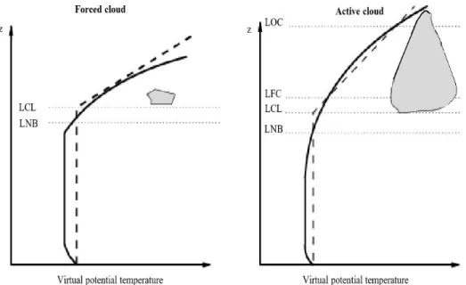
unless stated explicitly otherwise. At first the parcel starts rising and follows the dry adiabatic lapse rate. At a certain point the parcel reaches its level of neutral buoyancy (LNB), see figure 2.2. This means that the parcel has the same density as its environment, i.e. if it had no momentum it would remain at that height. But as the parcel has a velocity in the z-direction it overshoots the LNB. It eventually reaches the lifting condensation level (LCL), if it has enough momentum in the z-direction. This is the level where the parcel would become saturated, thus the level at which the cloud forms.

From here there are two possible scenarios. One is that the lapse rate of the environment is larger than the wet adiabatic lapse rate of the parcel. In this case the parcel remains negatively buoyant and the cloud will be limited in its growth. This is called a forced cloud and in this case the atmosphere is absolutely stable(figure 2.2 left part). In the other case however v is smaller than the wet adiabatic lapse rate. This means that the parcel is again positively buoyant if it reaches the level of free convection (LFC). This is the level where a a parcel of air lifted dry-adiabatically until saturated and saturation-adiabatically thereafter would first become warmer than its surroundings in a conditionally unstable atmosphere. To reach the LFC the parcel has to have enough vertical

Figure 2.1: Potential temperature lapse rates. Clouds will form when the lapse rate is between the dry- and wet-adiabatic lapse rate. Also depicted is the total specific humidity profile.

(9)

momentum when it reaches the LCL. As the parcel, which is now a cloud parcel, is positively buoyant again it continues to rise and condensate until another level is reached, the limit of convection (LOC). This is the level of neutral buoyancy for a saturated air parcel. At this level the temperature of the environment and the cloudy air parcel are once again equal. It is again possible that this level is overshot, and that the parcel penetrates into the inversion layer. The inversion layer serves as a “lid” on the mixed layer, and is a very stable layer. Eventually the parcel reaches a level where its momentum becomes negative and this marks the top of the cloud. In the process at cloud top there is mixing with the environment.

As the parcel penetrates into the inversion layer it is possible that air is entrained from the inversion into the cloud layer. This generally tends to lead to a deepening of the cloud layer. The formation of the cloud and the height it reaches depend on the forcing of the rising thermal, or as one could argue on the properties of the liquid water potential temperature and the total specific humidity. The larger the forcing the taller the cloud can become. One remark that has to be made is that the given explanation is highly idealized. The main reason for this is that the properties of the thermal are in reality not conserved. There is to a certain extent lateral mixing which leads to a bending of the profile of the rising parcel in figure 2.2 to the environmental curve.

With the aid of the buoyancy a energy quantity can be derived that is believed to be a measure for the vertical velocity in the cloud. This is the Convective Available Potential Energy (CAPE). It is also the maximum (kinetic) energy available to a rising parcel. The definition of CAPE is given by

(2.10)

Figure 2.2: Forced and active cloud development including appropriate levels. Solid line is the environmental lapse rate. Dashed line is the lapse rate of the rising parcel.

A=

∫

_LFCLOC Fbdz=

g

v

∫

LFC LOC

(10)

Between the limit of free convection and the limit of convection the buoyancy force is positive. That is why these are used as the limits of integration. When one assumes that all potential energy is converted into kinetic energy the following velocity scale results

(2.11) There are two major limitations to the use of CAPE. One being that lateral mixing and pressure effects are neglected, the other that the exact levels of LFC and LOC can make a big difference in the estimation of CAPE.

2.3.The Turbulent Kinetic Energy budget equation

An important parameter in the study of the ABL is the turbulent kinetic energy (TKE) budget. This is so because the TKE budget is a measure of turbulence intensity and as such directly related to the transport of momentum, heat and moisture through the atmosphere. Grant & Lock (2004) state that understanding what determines the magnitudes of the terms in the TKE budget is a key element in understanding turbulent flows and thus the ABL.

The TKE budget for a stationary, horizontally homogeneous boundary layer is

(2.10) The brackets denote as before an ensemble averaged mean. In this equation the first term is production of TKE by mean shear, the second term is a buoyancy production term. The third and fourth term (between brackets) are vertical transport (redistribution) respectively a pressure-velocity correlation term which is also responsible for transport. The last term is responsible for molecular transport of TKE and is given by −〈u 'i∂2u'i

∂x2j 〉. As one can see the TKE budget equation is nothing more than a summation of production and loss terms that are, in this special case, at equilibrium. In convective situations the buoyancy flux is the most important producer of TKE. This is also why CAPE is considered to be of use in the ABL.

2.4.Large Eddy Simulation

In the modeling of the ABL there are eddies on a variety of length scales. They range from the Kolmogorov microscale (order of magnitude 1 mm) to the scale of the boundary layer (order of magnitude 1 km). The energy in a turbulent flow is transported in what is termed the cascade-process. In this process energy is transported to successively smaller eddies until eventually on the smallest eddy scale the energy is dissipated through viscous forces. To simulate a turbulent flow one would favor the use of direct numerical simulation (DNS), where all turbulent scales are resolved. However, as this would require 1018_{gridpoints (x, y and z-direction) for a cubicle of air}

∂e ∂t=−〈u' w '〉 ∂ 〈 u〉 ∂z  g v ,0 〈w 'v'〉− ∂_∂_z〈w ' e〉1_∂ 〈 w ' p'〉 ∂z −=0 w_CAPE=

_

2A

(11)

with a dimension of 1 km3_{, this is computationally not feasible. Common practice therefore is to}

look at the large scale eddies and resolve them explicitly.2_{The smaller eddies are then parametrized,}

as opposed to DNS where all eddies are resolved. This is what is termed LES. The rationale for explicitly resolving the largest eddies is that they can be thought of as being dependent on the large scale forcings of the environment. They are also responsible for the transport of the bulk of heat, moisture and momentum. For the smaller scale eddies it is generally assumed that they behave independently and thus can be parametrized without loss of applicability of the (LES)-model. The closure that is needed for the sub-grid scale eddies is simpler than a closure scheme for the macro structure because the micro (or sub-grid) scale has a uniform structure. Furthermore simulation results show that the macro structure is rather insensitive to the chosen sub-grid closure (Nieuwstadt (1998)).

(12)

3.Methodology

In this chapter the research aim will be discussed. The first paragraph gives a short overview of the relevant large scale forcings and initial profiles that are specified under BOMEX, or for that matter any LES run of the ABL. The second paragraph focuses on the parameters that we think have the most influence on the mean profiles of the simulations. As a conclusion to this chapter we will formulate hypotheses regarding the outcome if one changes the initial data.

3.1.Initial set up

For any LES to be run inputs have to be specified. These include initial profiles of the mean temperature and humidity and the horizontal velocity components. Furthermore large scale forcings, describing processes that act on a larger scale than the domain that is considered in the LES, need to be taken into account. These forcings include the radiative cooling of the atmosphere, the subsidence velocity, geostrophic winds3_{and large scale low-level drying due to advection.}

Finally consideration has to be given to the surface fluxes. Therefore the sensible and latent heat and the momentum surface flux are prescribed.

By imposing an initial set up to the model the first two hours are generally considered to be fairly useless as the model is in a so called “spin up” state. This presents itself most clearly in the strong peak in cloud cover that appears after one hour (see Siebesma et al. (2003)). The spin-up comes about because initially there is no resolved-scale turbulence that can generate horizontal variability in temperature and humidity. Therefore the first clouds all arise simultaneously, but after two hours this behavior dampens out as not all clouds arise simultaneously any longer.

In BOMEX the initial profiles are derived from measurements whereas the large-scale forcings are based on budget studies (Holland and Rasmusson (1973)).

3.2.Important parameters

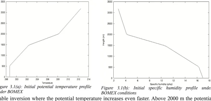
Having described the parameters used in the set up of the LES it is now time to pay attention to the most important parameters. As we are studying the mean profiles and the way they transport energy through the ABL this dictates which parameters we will change. Obviously the mean profiles itself are of great importance, as a change in the initial profile is likely to impact the results from the LES. In figure 3.1(a) the mean (liquid water) potential temperature profile is sketched. There are four distinct parts. In the first 500 m a well mixed layer is supposed, where the potential temperature stays the same, the mixing is due to turbulence. Between 500 and 1500 m the potential temperature raises due to the formation of clouds. Then between 1500 and 2000 m we find a strong 3 The geostrophic wind is the horizontal wind for which the Coriolis acceleration balances the horizontal pressure

(13)

stable inversion where the potential temperature increases even faster. Above 2000 m the potential temperature raises in the same fashion as in the clouds.

The initial profile for the specific humidity is depicted in figure 3.1(b) and follows a similar, but reversed, pattern (four distinct pieces) as the temperature. There are several adjustments possible in the initial profiles. First one can shift the total profile. Also one can change the lapse rate between 500 and 1500 m. Finally the altitude of the cloud base and the inversion base can be altered.

Another important parameter is the (large scale) subsidence. This downward motion of air acts as a limitation on the formation of clouds. The stronger the downward motion the lower clouds will form and the smaller they become. We therefore believe that this can act as a strong influence on the mean profiles. The large scale subsidence can emerge as part of the Hadley circulation, which is depicted in figure 3.2. As we study the second cloud type from the left in the Hadley circulation it is obvious that the subsidence is not limited to the Hadley circulation. An area of high pressure in itself also produces subsidence.

We believe the parameters discussed thus far can have a direct influence on the mean profiles. A more extensive understanding will be developed in chapter 4. Other parameters are naturally of influence to cloud formation and stability of the ABL. These include the surface fluxes, radiative cooling and large scale advection. They are very important but by changing them the starting point and further evolution of the simulation are changed. We are most interested if a more subtle change in initial parameters can alter the outcome of the mean profiles. The impact of radiative cooling is at best responsible for small differences. In a recent study (Axelsen (2005)) where the radiative cooling was set to zero, similar results to BOMEX were found. This study is however limited because the runtime of the simulations was rather short. The rest of our research is therefore limited to the initial profiles of temperature and specific humidity and the large scale subsidence.

Figure 3.1(b): Initial specific humidity profile under BOMEX conditions

Figure 3.1(a): Initial potential temperature profile under BOMEX

(14)

3.3.Hypotheses

It is relevant and useful to deduce hypotheses of what we expect to happen when we alter the initial profiles and the subsidence. A common approach in the study of turbulence is to resort to scaling laws and similarity theory. Similarity theory uses dimensional analysis to obtain relationships in non-dimensional form, with the goal to reveal scaling laws. This gives, besides a qualitative description, a more quantitative approach as to why we expect certain effects and how large they will be. This is an important way to improve on our knowledge of shallow cumulus. There is little theory that describes the impact of altering the profiles and large-scale subsidence. A recent study by Grant & Lock (2004) based on similarity theory by Grant & Brown (1999) used the following relation as a method for obtaining conditions for steady shallow cumulus

(3.1) where A stands for the convective available potential energy (CAPE), w_∗stands for the sub-cloud layer convective velocity scale defined by w∗=

g zlcl

v ,0 w 'v'

1/3

. zlcl and zcld are the height of the lifting

condensation level respectively the depth of the layer between cloud base and the base of the inversion. They further derive that

(3.2) This looks like the most promising (theoretical) avenue to assess whether shallow cumulus stays

w_∗ A1/2≈0.2 z_lcl z_cld w_∗ A1/2~ z_lcl z_cld 6/7

Figure 3.2: The Hadley circulation, the order of magnitude of the large-scale subsidence is about 1 cm/s. Ev is

(15)

stable. One problem that needs to be solved is how they deduce a linear-law respectively a 6/7-law for the same quantity. Grant and Lock indicate that the fomer relation is derived from a small number of simulations and that the latter has wider applicability.

Research by Neggers et al. (2004) shows there is an equilibrium solution for shallow cumulus. They use a simplified mass flux closure, which introduces a moisture-convection feedback. They achieve this by retaining the cloud fraction in their closure. Neggers et al. give numerical results of their model. An interesting result of their paper is that for a constant (sea) surface temperature the subsidence velocity has hardly any influence on the mixed layer humidity.

It is interesting to see if the above mentioned scalings work under the initial profiles we are considering.

(16)

4.Sensitivity experiments

This chapter discusses the actual set up of the adjustments that have been made to the standard BOMEX case, which will be discussed shortly in paragraph 4.1. Paragraph 4.2 discusses the shift in initial profiles, whereas paragraph 4.3 gives an overview of the adjustment of the lapse rate in the cloud layer. Paragraph 4.4 concludes with the adjustment of the large scale subsidence velocity.

4.1.The BOMEX case

The BOMEX case is one of the oldest and most studied weather cases in the meteorological world. It was conducted in June 1969 near the coast of Barbados. At that time it was the most sophisticated and costly effort to understand weather in general and trade wind regimes in particular. In the Barbados region typical trade wind cumulus is frequently observed and this was also the case during phase 3 of BOMEX. One of the desirable features of this phase is that it was remarkably steady. Furthermore there was no observed precipitation or mesoscale fluctuations in fluxes. BOMEX was conducted on a square of approximately 500 x 500 km. A detailed description can be found in Holland and Rasmusson (1973)

In most recent (LES)-studies that use BOMEX the average profiles of two days of the most northern ship of the BOMEX square are used. This is so because averaging over greater temporal or spatial domains levels out the inversion that is found on the individual profiles, see e.g. Siebesma et al. (2003). The actual data were obtained from rawinsondes, which produced observations for temperature, wind velocity, humidity and cloudiness. They were complemented with surface level data taken by ships and buoys.

In the present study the simulation has a horizontal domain of 6.4 x 6.4 km, with the grid points evenly spaced at 100 m intervals. In the vertical (z-) direction we have a total of 80 grid points with a mutual distance of 40 m, leading to a height of 3200 m.

4.2.Shifting the initial profile

The initial profiles for temperature and humidity were discussed in section 3.2. When shifting the profiles for l and qt one should expect that cumulus clouds will still form. When the air becomes

warmer while q_t remains constant there is increased evaporation leading to clouds that should form higher. The opposite is true for a lower l. Here one should expect to see clouds at lower altitudes

as a rising air parcel is saturated earlier.

When the q_t profile is changed something similar is expected to happen. A higher total humidity should lead to clouds forming lower because the air is saturated earlier.

(17)

thereafter positively buoyant again. Once the parcel reaches the LOC it is negatively buoyant but due to the overshoot it will entrain some air of the environment, thereby deepening the cloud layer. Because the warmer air then leads to faster evaporation (due to the higher overall temperature) the logical consequence is that the cloud top of the colder profiles should be higher than that of the warmer profiles.

Case name Surface temp

(K) _{500 m (K)}l at _{1460 m (K)}l at Runtime(hours) BOMEX BOMEX 299.1 298.7 302.3 36 Shift l +0.3% SHIFTT+3 300.0 299.6 303.7 36 +0.6% SHIFTT+6 301.2 300.8 304.5 36 +1.0% SHIFTT+10 302.1 301.7 305.3 36 -0.3% SHIFTT-3 298.2 297.8 301.9 36 -0.6% SHIFTT-6 297.3 296.9 301.0 36 -1.0% SHIFTT-10 296.1 295.7 299.3 36

Table 4.1: Shifted temperature profile. Note that l remains unchanged, not mentioned values are similar to BOMEX.

Finally we can make some remarks about l in the cloud layer. We expect, following the same reasoning as above, that the warmer profiles lead to smaller clouds (i.e. smaller vertical extent). In these clouds however the lapse rate is expected to be equal. For the humidity profile there should be no apparent change in the lapse rate either.

The l profile was shifted by 0.3%, 0.6% and 1% in either direction (see table 4.1), whereas the

qt profile was shifted by 1%, 2% and 4% in either direction (see table 4.2). The shifts were chosen

to disturb the initial profiles significantly but not that much that clearly irrelevant scenario's would occur. To evaluate whether a scenario is relevant typical (average) surface specific humidity and temperature were considered.

Typical specific humidity (at sea level) varies considerably over the surface of the earth. The largest values being found in the tropics (~20 g/kg) and the lowest values near the poles (~2 g/kg). The temperature variations follow the same pattern and lie between 265-305 K. The chosen values are well within these ranges and also within (sub)tropical ranges.

(18)

Case name q_t at 20 m (g/kg) q_t at 500 m (g/kg) q_t at 1460 m (g/kg) Runtime (hours) BOMEX BOMEX 16.97 16.33 10.82 36 Shift q_t +1% SHIFTQ+1 17.14 16.50 10.99 36 +2% SHIFTQ+2 17.31 16.67 11.16 36 +4% SHIFTQ+4 17.65 17.01 11.50 36 -1% SHIFTQ-1 16.80 16.16 10.65 36 -2% SHIFTQ-2 16.63 15.99 10.48 36 -4% SHIFTQ-4 16.29 15.65 10.14 36

Table 4.2: Shifted humidity profile. Note that qt remains unchanged, not mentioned values are similar to BOMEX.

4.3.Adjusting the lapse rate

Besides shifting the initial profiles l and l can also be adjusted. As these are adjusted we expect that this should be persistent. As BOMEX is stable with respect to the lapse rate there is no a priori knowledge that does change this expectation for a changed lapse rate.

When the lapse rate is changed there is more entrainment so we expect a deepening of the cloud layer with time. By increasing the lapse rate we expect that the cloud layer deepens faster, because of the faster rise in temperature. By increasing the humidity lapse rate the atmosphere in the cloud layer becomes drier. We therefore expect that the clouds will evaporate more quickly, thereby becoming less deep. As to the cloud base we expect no changes.

The adjustment of the lapse rates was made for the humidity and temperature. The percentage changes were +10%, +20%, +30% and -10% (see table 4.3 respectively 4.4). The main rationale for increasing l (as opposed to decreasing it) is that we expect to see a greater effect from warmer profiles, because this brings the lapse rate closer to the moist adiabat and thus closer to absolute stability, where no clouds will form.

Case name Surface temp

(K) _{500 m (K)}l at _{1460 m (K)}l at Runtime(hours) BOMEX BOMEX 299.1 298.7 302.3 36 l adjustment +10% LRT+10 299.1 298.7 302.7 36 +20% LRT+20 299.1 298.7 303.0 36 +30% LRT+30 299.1 298.7 303.4 36 -10% LRT-10 299.1 298.7 302.0 36

(19)

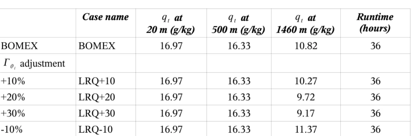
Case name q_t at 20 m (g/kg) q_t at 500 m (g/kg) q_t at 1460 m (g/kg) Runtime (hours) BOMEX BOMEX 16.97 16.33 10.82 36 l adjustment +10% LRQ+10 16.97 16.33 10.27 36 +20% LRQ+20 16.97 16.33 9.72 36 +30% LRQ+30 16.97 16.33 9.17 36 -10% LRQ-10 16.97 16.33 11.37 36

Table 4.4: Adjustment of qt. Note that the sub-cloud layer is similar to BOMEX for all simulations.

4.4.Subsidence velocity

The subsidence velocity acts as a large scale forcing on the total grid. We expect therefore that for increasing subsidence velocity clouds will become less pronounced. The cloud base will most likely be at the same height and as the initial profiles remain the same the lapse rate will most likely remain unchanged.

On the other hand it can be argued on the basis of equation (2.7)-(2.9) something has to change in the lapse rate. Because the situation is considered stable (after spin-up) the time derivative can be set to zero. This implies that, as the only change that has been made to (2.9) considers the subsidence (w-)velocity, and the lapse rate is constant in time, the lapse rate should adapt to the changed subsidence. If this is not the case one should expect that the other terms in (2.9) show adaptation, or the simulation cannot be considered stable.

With respect to the inversion we expect that a larger subsidence leads to a lower cloud. Because of the larger subsidence the inversion is pushed down. So as a consequence, the larger the subsidence the smaller the cloud will be in time. The changed subsidences are given in table 4.5 (maximum value at 1500 m, according to Siebesma et al. (2003)). The changes are substantial but in the typical range of subsidence velocities of 0.2-1 cm/s.

Subsidence

change Case name 1500 m (cm/s)w at Subsidence change Case name 1500 m (cm/s)w at

BOMEX -0.650 BOMEX -0.650

+10% SUB+10 -0.715 -10% SUB-10 -0.585

+20% SUB+20 -0.780 -20% SUB-20 -0.520

+30% SUB+30 -0.845 -30% SUB-30 -0.455

(20)

5.Results & Discussion

This chapter will focus on the results that are obtained from the simulations. The first paragraph will focus on the actual results and tries to give explanations for the obtained data. Paragraph 5.2 will link our results with the existing literature and will focus on appropriate scaling laws that were discussed in chapter 2. The final paragraph concludes and gives some recommendations for future research.

5.1.Results from the simulations

We display the profiles that result from the simulations in the same order as in chapter 4. We will therefore start with the shifted profiles. As the simulations are run for 36 hours we could show a plot of the mean profiles every 30 minutes of the simulation. As this would result in a very lengthy report we will limit the figures to plots of the mean profiles 6 and 28 hours. Divergences from these profiles in other hours of the simulation will naturally be discussed. In the figures q_l and q_t are shown along with l. Furthermore a plot of the development of l in the cloud layer over time is shown. The calculation of l is made on the basis of an interpolation between two points in the cloud layer. These points are chosen visually for every simulation to be certainly within the cloud layer. This is done on the basis of the l plots, where the lapse rate appears to be uniform. A further

support for the choice for these points is then obtained by looking at the q_l plots to see if there is indeed a (substantial) amount of liquid water present.

As is clear from figure 5.1 there are definite effects from shifting the initial l profile. Most

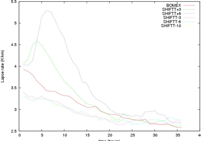
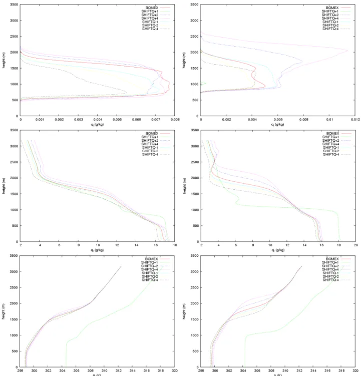
notably there is an effect on the cloud top. For the whole simulation the cloud top of the colder profiles is above the cloud top of the warmer profiles. This can be understood, since the warmer profiles are fully evaporated at a lower altitude. A colder air parcel starts to condensate earlier. This can be seen in the lower right, where the cloud base of the colder profiles is lower than that of the warmer profiles. But as the condensation takes place at a lower temperature the evaporation is slower. Therefore the cloud top will be higher than that of a relatively warm profile. This is exactly what is the case in this shift. It is interesting to note that this leads to a faster drying of the atmosphere, also in the sub-cloud layer. Apparently there is a feedback mechanism from the cloud layer to the sub-cloud layer. Initially l of the warmer profiles is substantially higher than that of the cold profiles. With time (see figure 5.2) all lapse rates (except for the +1% case) converge to an average value of 2.7 K/km. Note that the -1% case is terminated before the end of simulation. This is due to the fact that the cloud layer develops over the height of the grid (i.e. above 3180 m). The +1% case does not develop any active cumulus and is not studied further.

(21)

The second profile shift that we considered was a shift in the humidity profile. The profiles after 6 and 28 hours of simulation are shown in figure 5.3. What immediately draws attention is the strange shape of the +1% profile. It is not known what has caused this shape, but as is apparent from the liquid water content, no clouds are formed in this case. We will therefore neglect this case, although it is remarkable that the +2% and +4% cases do not exhibit this behavior. The effect on the temperature is evident though less pronounced than the effect of temperature on humidity. The same reasoning applies here as in the previous case. Also the moisture feedback between cloud and

Figure 5.1: Left top to bottom: ql, qt and l for the shifted l profiles after 6 hours of simulation. Right top to

(22)

sub-cloud layer seems to be present. After 6 hours the drier profiles have caused a decline in the surface temperature, whereas the more humid profiles have increased the surface temperature.

The cloud base is in this set of simulations very steady. Among the different simulations there is hardly any difference, although with time the sub-cloud layer deepens. This is understandable as the surface temperature increases, which in turn is due to the large scale low-level drying. This is 1.2 g/kg/day which is approximately the shift that can be deduced from the two middle figures in figure 5.3. The inversion height of the drier profiles gradually lowers as was expected because the cloud parcels have less water content and are thus fully evaporated lower in the atmosphere as opposed to the humid profiles where the cloud layer gradually deepens. The lapse rate again decreases with time to a value of 2.70 K/km as can be seen in figure 5.4. To form some sort of criterion of the convergence we can take the bandwidth of the lapse rate at a certain time. For figure 5.3 as well as figure 5.4 the convergence is evident, because the bandwidth at hour 12 is much larger than it is after 30 hours of simulation. What is furthermore interesting is that in the l simulations the

colder initial profiles are much more coherent over the simulation horizon than the warmer profiles

Figure 5.2: Lapse rate for the shifted l profiles. Note that the +1% case is not displayed, because the cloud depth was

(23)

Having seen the results from the shifted profiles we now turn attention to the profiles with the adjusted l and qt. Figure 5.5 displays the results for l. After 6 hours the temperature profiles are still somewhat in line with the original perturbation. However after 28 hours the lapse rate is at the same level as in the previous simulations (~2.70 K/km) whereas the cloud base and cloud top are shifted. Evidence of the feedback mechanism is also present as the surface

Figure 5.3: Left top to bottom: ql, qt and l for the shifted qt profiles after 6 hours of simulation. Right top to

(24)

temperature has changed. Also there is a drying tendency in the atmosphere and the cloud depth for the colder profiles has become deeper than that of the warmer profiles. This can again be understood in terms of the evaporation. The change of l over the simulated time is shown in figure 5.6. Although there is initially a large difference in the lapse rates after about 10 hours of simulations it is at the same level for all simulations. However after this time there is no further convergence. This leads to the conclusions that there are forcings within the model that act to develop a certain lapse rate. To achieve this lapse rate other parameters are adjusted, such as the cloud and inversion base and the surface temperature and humidity. The reason why the model has such a strong preference for this lapse rate is unknown.

Figure 5.4: Lapse rate for the shifted humidity profiles. Note that the +1% case is not displayed, because of the fact no clouds were formed. The strong convergence of the lapse rate is readily evident.

(25)

Now that we have looked at the adjustment of l we can focus on the adjustment of qt. As is evident from figure 5.6 the +30% profile crashed after 21 hours of simulation. It is not readily apparent why this happened because the cloud top was not very high and there were still cumulus clouds present at hour 20. It might have something to do with the top of the domain, where there is a sponge layer to dampen disturbances. The humidity profile probably had to much influence from this sponge layer. An indication for this is that there is a clear swing in the humidity profile at 2000 m at 28 hours which gradually develops over the simulation horizon.

Figure 5.5: Left top to bottom: q_l_,q_t_and__l_{for the adjusted}l after 6 hours of simulation. Right top to bottom:

(26)

Furthermore one can notice that the same effects as in the previous simulations are present, albeit less pronounced than in the case of a change in the temperature profile. After 6 hours the change in the humidity profile is still discernible and the effect on temperature is still small. After 28 hours the lapse rate for temperature is on its usual level. When one compares the temperature and humidity adjustment, the temperature seems to have a greater influence on the humidity than the other way around. However this is purely a qualitative notion and needs to be tested further. The lapse rate decreases in a similar fashion as in the other profiles to the value of 2.70 K/km.

Lastly we look at the adjustment of the subsidence. What directly draws attention is the similarity of the surface temperature. Here there is no feedback present from the clouds to the sub-cloud layer. Or better said, the adjustment of the subsidence velocity gives no direct influence on the surface values. This strengthens the belief that there is some kind of moisture feedback, because when we changed one of the two values that are of direct influence on the initial profile there were changes in the sub-cloud layer values of temperature and humidity.

The only effect that can be deduced from the change in the subsidence velocity is an effect on the base of the inversion. This effect is as expected, the stronger the subsidence velocity the lower the

Figure 5.6: Lapse rate over time for the adjusted l. The strong convergence of the lapse rate in the first 10 hours is

(27)

cloud layer will become (or: the inversion will be pushed downwards stronger). There is no effect on the lapse rate, and there was no effect on the fluxes is well. This is surprising in light of the discussion in chapter 4. What is also strange is the fact the +20%, -10% and -20% profiles crash after 24 hours. There is once again no apparent reason, especially because the +/-30% adjustments do not crash. It might be attributed to the top level value of temperature and humidity. Concluding one can say that the trend is persistent among all simulations where the initial profiles were changed that there is a moisture feedback. This was maybe unexpected, but confirms the

Figure 5.7: Left top to bottom: q_l_,q_t_and_l for the adjusted qt after 6 hours of simulation. Right top to bottom: ql

(28)

parametrization proposed by Neggers (2004). Furthermore it is interesting to note that the change in lapse rate is not persistent. In the conclusion we will elaborate on this matter.

Figure 5.8: Lapse rate over time for the adjusted humidity lapse rate. The strong convergence of the lapse rate is readily evident. The +30% adjustment crashed after 21 hours of simulating.

Figure 5.9: Lapse rate over time for the adjusted subsidence velocity. The strong convergence of the lapse rate is evident, although the +10% adjustment seems to be a bit off . +20%, -10% and -20% crash after 21 respectively 24 hours.

(29)

Figure 5.10: Left top to bottom: liquid water content, total water content and liquid water potential temperature for the adjusted subsidence after 6 hours of simulation. Right top to bottom: liquid water content, total water content and liquid water potential temperature for the subsidence after 28 hours of simulation.

(30)

5.2.Scaling laws

Here we will shortly evaluate the discussed scaling laws in chapter 3. We will start with the Grant & Lock (2004) scaling law, which is based on the cloud depth, CAPE and sub-cloud layer velocity scale. The different values of the cloud base, zlcl, cloud depth, zcld, CAPE and sub-cloud layer

convective velocity are given in table 1, for the 6 and 28 hour averages. What is readily apparent is that the CAPE develops with time. Especially for active clouds the difference between the 6 and 28 hour CAPE is significant. In contrast the sub cloud convective velocity scale is rather constant during the simulation time. The cloud depth tends to deepen for active clouds, whereas the sub-cloud layer deepens as well. This is in accord with the findings in the previous paragraph. More active clouds carry a greater CAPE and this becomes more pronounced over the duration of the simulation.

The proposed scaling is graphed in figure 5.11 for four points in time (6-7, 12-13 27-28 and 35-36 hours). It is apparent that the proposed scaling seems to work reasonably well. Concluding we can say that the scaling evolves with time but is clearly present. The evolvement with time is surprising because Grant & Lock propose their scaling as being independent of time and characteristic for shallow cumulus. Furthermore it is interesting that after about 20 hours of simulation the scaling is stable with respect to time, a linear fit confirms this as the standard error drops considerably with time. There is thus a limit on this scaling.

Figure 5.11: Scaling for different times in the simulation. With time the scaling becomes more constant. The scaling is persistent over the whole simulation horizon however. Linear scaling is plotted, the 6/7-scaling gave similar results.

(31)

Table 6.1: Overview of the different simulations and key parameters. Cloud base (z_lcl), depth of layer between cloud base and base of the inversion (z_cld), CAPE and sub-cloud layer convective velocity scale, w*. For some

simulations values are missing. This is due to a crash (e.g. subsidence +20%) or the fact that no clouds were present at that time (shift (theta) +0.6%). Two simulations are not represented at all as they produced no cumulus clouds. Those are the +1% shift of the humidity profile and the +1% shift of the temperature profile.

hour z_lcl z_cld CAPE w * hour z_lcl z_cld CAPE w *

BOMEX Lapse rate (theta) +10%

6 500 1980 41.56 0.657 6 500 1860 33.12 0.657

28 740 2060 79.79 0.749 28 700 1860 62.23 0.735

Shift (theta) -0.3% Lapse rate (theta) +20%

6 420 2380 59.52 0.620 6 500 1900 27.84 0.657

28 700 2540 168.73 0.735 28 700 1700 48.14 0.735

Shfit (theta) -0.6% Lapse rate (theta) +30%

6 420 2500 82.35 0.620 6 460 1660 22.39 0.639

28 700 2900 215.87 0.735 28 660 1740 39.54 0.720

Shift (theta) -1% Lapse rate (theta) -10%

6 380 2820 127.17 0.600 6 540 2140 52.10 0.674

28 740 2100 98.84 0.749

Shift (theta) +0.3% Lapse rate (q) +10%

6 580 1780 36.78 0.690 6 500 1820 42.92 0.657

28 740 2060 84.29 0.748 28 740 2100 72.73 0.749

Shift (theta) +0.6% Lapse rate (q) +20%

28 780 2020 54.81 0.761 6 540 2100 41.40 0.674

28 780 1940 60.53 0.762

Shift (q) +2% Lapse rate (q) +30%

6 500 2140 47.93 0.657 6 540 1940 42.97 0.674

28 740 2500 112.92 0.749

Shift (q) +4% Lapse rate (q) -10%

6 460 2140 53.53 0.639 6 540 1980 43.20 0.674 28 740 2620 140.26 0.748 28 740 2100 83.60 0.749 Shift (q) +1% Subsidence +10% 6 540 1940 41.47 0.674 6 500 1980 40.92 0.657 28 740 2100 71.26 0.749 28 740 1940 60.49 0.749 Shift (q) -2% Subsidence +20% 6 540 1900 38.52 0.674 6 500 1940 37.92 0.657 28 740 2020 61.27 0.749 Shift (q) -4% Subsidence +30% 6 580 1820 36.32 0.690 6 500 1820 34.84 0.657 28 740 1780 49.14 0.749 28 740 1620 30.26 0.749 Subsidence -30% Subsidence -10% 6 500 2060 48.12 0.657 6 500 2340 45.07 0.657 28 740 2420 131.44 0.749 Subsidence -20% 6 500 2060 45.76 0.657

(32)

6.Conclusion

The adjustment of the different initial profiles has a clear effect on the mean profiles over the duration of the simulation. The most noteworthy is the feedback effect that a change in the lapse rate (humidity as well as temperature) has. This is likely due to entrainment from the cloud layer to the sub-cloud layer. Furthermore, this study started out to see if a different lapse rate could be obtained by changing the profiles.

As we have seen it is not possible to adjust the lapse rate to a new value because with time the lapse rate converges to a value of about 2.70 K/km. There is no apparent reason, nor is there any observational evidence that this must be the case. There are numerous lapse rates observed in shallow cumulus clouds. This is an interesting avenue for further research. Lastly there are some effects that could be expected on the basis of the altered profiles. There are no surprises within these results. As the initial profiles are sometimes disturbed quite a bit the model has a large capability in restoring a cumulus cloud deck. This is for example the case in the shift of the temperature profiles. After a number of hours the cumulus clouds are again present where at the start no such clouds were present.

We can notice two more things. The simulation is more sensitive to shifts in temperature than humidity. With respect to the lapse rate a similar result is found. However this conclusion is a bit far fetched as determining what is an appropriate and comparable shift is difficult. The second is that the change in large scale forcings (only the subsidence velocity has been adjusted) has no effect on the sub-cloud layer or the lapse rate. There is also no change in fluxes that stabilizes the change of the subsidence velocity. What does counteract the change in subsidence is not known.

Besides the mean profiles we have also looked at a scaling law. The scaling law by Grant & Lock (2004) gives a condition for steady cumulus. From our simulations the scaling law works good. Especially later in the simulation the scaling converges and becomes steady. The most notable thing is the rising of the cloud base (or so to speak the deepening of the sub-cloud layer). A weakness with regard to the model is that the temperature and humidity at the top of the domain cannot be adjusted. The specification in the initial profile determines these values for the whole simulation. Therefore at the top of the profiles large swings can be observed that are “model-driven”. It might be interesting to see what happens when these values could be changed.

This study has in our opinion raised more questions than answered. It has however demonstrated that the scaling of Grant & Lock works well and that the change in initial profiles does influence the dynamics of the ABL. Further research on large scale forcings might tell us more about the underlying processes that determine the dynamics of the cloud layer, and with that the lapse rate.

(33)

It is very interesting to see that this model has a clear preference for a certain lapse rate (2.70 K/km). This preference has such a large influence that, when an initially different l is specified this with time evolves back to the fixed value. Furthermore it is interesting to note that initially BOMEX is not in steady state. This is most clear from the shifted l profiles where the colder

profiles are more steady with respect to lapse rate than BOMEX or the warmer profiles.

Another area which is interesting for conducting further research is the moisture feedback that is present when the cloud dynamics are slightly perturbed. It was hypothesized that such a feedback should be present and our study has demonstrated that this is indeed the case.

(34)

Bibliography

Augustein, E., Riehl, H., Ostapoff, F. and V. Wagner, Mass and energy transports in an unditurbed Atlantic Trade-wind flow, Monthly weather Review 101, pp. 101-111, 1973

Cuijpers, J.W.M. and P.G. Duynkerke, Large Eddy Simulation of Trade-wind cumulus clouds, Journal of Atmospheric Science, 50 pp. 3894-3908, 1997

Garratt, J.R., The atmospheric boundary layer, Cambridge University Press, Cambridge, 1992

Grant, A.L.M. and A.R. Brown, A similarity hypothesis for shallow-cumulus transports, Quarterly Journal of the Royal Meteorological Society, 125 (558), pp. 1913-1936, 1999

Grant, A.L.M. and A.P. Lock, The Turbulent Kinetic Energy budget for shallow cumulus convection, Quarterly Journal of the Royal Meteorological Society, 130 (597), pp. 401-422, 2004

Holland, J.Z. and E.M. Rasmusson, Measurements of Atmospheric mass, energy and momentum budgets over a 500-kilometer square of tropical ocean, Monthly Weather Review 101, pp. 44-55, 1973

Axelsen Looijen, S., The role of relative humidity on shallow cumulus dynamics; results from a Large Eddy Simulation Model, Master's Thesis, Utrecht University, Utrecht, 2005, http://www.phys.uu.nl/~0321060/uni/cumulusles.pdf

Negger, R.A.J., Shallow Cumulus Convection, Proefschrift Wageningen Universiteit, Ponsen & Looijen, Wageningen, 2002

Neggers, R.A.J., Stevens, B. & J.D. Neelin, An equilibrium model for marine shallow cumulus convection, 16th_{symposium on Boundary Layer and Turbulence, P1.3, 2004}

Nieuwstadt, F.T.M., Turbulentie: theorie en toepassingen van turbulente stromingen, Epsilon Uitgaven, Utrecht, 1998

Roode, S. de, Clouds, course material for MO404, Utrecht University, http://www.phys.uu.nl/~roode/CLOUDS_COURSE/Clouds.pdf, 2004

(35)

Siebesma, A.P., Bretherton, C.S., Brown, A., Chlond, A., Cuxart, J., Duynkerke, P.G., Jiang, H., Khairoutdinov, M., Lewellen, D., Moeng, C.H., Sanchez, E., Stevens, B. and D.E. Stevens, A Large Eddy Simulation Intercomparison study of shallow cumulus convection, Journal of the Atmospheric Sciences, 60 (10), pp. 1201-1219, 2003

Soares, P.M.M., Miranda, P.M.A., Siebesma A.P. & J. Teixeira, An eddy-diffusivity/mass-flux parametrization for dry and shallow cumulus convection, Quarterly Journal of the Royal Meteorological Society, 130, pp. 3365-3383, 2004

Stevens, B., Scaling laws for shallow moist convection, 16th_{symposium on Boundary}

Layers and Turbulence, P1.3, 2004

Stull, R.B., An introduction to boundary layer meteorology, Kluwer Academic Publishers, Amsterdam, 1988

Tennekes, H. and J.L. Lumley, A first course in Turbulence, MIT Press, Cambridge (MA), 1972