The deployment of extra relay nodes around the sink in order to solve the energy imbalanced problem in Wireless Sensor Networks

(1)

UNIVERSIDAD

POLITÉCNICA DE

C

ATALUÑA

M

ASTER

T

HESIS

The deployment of extra relay nodes

around the sink in order to solve the

energy imbalanced problem in

Wireless Sensor Networks

Author:

Hanz Rodríguez Ramos

Supervisor: Jose M. Barcelo-Ordinas

A thesis submitted in fulfillment of the requirements for the degree of Master in Innovation and Research in Informatics

in the

Computer Networks and Distributed Systems FIB - Barcelona School of Informatics

(2)

(3)

iii

Declaration of Authorship

I, Hanz Rodríguez Ramos, declare that this thesis titled, “The deployment of extra relay nodes around the sink in order to solve the energy imbalanced problem in Wireless Sensor Networks” and the work presented in it are my own. I confirm that:

• This work was done wholly or mainly while in candidature for a re-search degree at this University.

• Where any part of this thesis has previously been submitted for a de-gree or any other qualification at this University or any other institu-tion, this has been clearly stated.

• Where I have consulted the published work of others, this is always clearly attributed.

• Where I have quoted from the work of others, the source is always given. With the exception of such quotations, this thesis is entirely my own work.

• I have acknowledged all main sources of help.

• Where the thesis is based on work done by myself jointly with others, I have made clear exactly what was done by others and what I have contributed myself.

Signed: Date:

(4)

(5)

v

UNIVERSIDAD POLITÉCNICA DE CATALUÑA

Abstract

Faculty Name

FIB - Barcelona School of Informatics

Master in Innovation and Research in Informatics

The deployment of extra relay nodes around the sink in order to solve the energy imbalanced problem in Wireless Sensor Networks

by Hanz Rodríguez Ramos

Wireless sensor networks are an emerging technology that has recently gained attention for their potential use in many applications such disaster management, combat field reconnaissance, border protection, object local-ization, harbors, coal mines, and so on.

Sensors in these kind of applications are expected to be remotely de-ployed and to operate autonomously in unattended environments.

Since sensors typically operate on batteries and are often deployed in harsh environment where human operators cannot access them easily, much of the research on wireless sensor networks has focused on the energy de-pletion in order to achieve energy efficiency to extend the network lifetime. In multihop wireless networks that are often characterized by many to one traffic patterns, it is very common to find problems related to energy depletion. Along the network, sensors experiment different traffic intensi-ties and energy depletion rates. Usually, the sensors near the sink tend to deplete their energy sooner because they act as data originators and data relayers and are required to forward a large amount of traffic of the most remote sensors to the sink while the sensors located in the periphery of the network remain much of the time inactive.

Therefore, these sensors located close to the sink tend to die early, leav-ing areas of the network completely disconnected from the sink reducleav-ing the functional network lifetime.

In order to achieve equal power consumption at different levels of our network, we have decided to add extra relay nodes to reduce and balance the traffic load that normal nodes have to carry. As mentioned above, each level within the network faces a different amount of traffic, which becomes more intense as we approach the interior levels. This behavior causes that the external nodes, with less traffic to handle, stay more time at rest while the nodes in the inner rings face a great amount of traffic which forces them to be more active, generating a more accelerated exhaustion, reason why nodes located in the inner rings exhaust its battery faster causing the life-time of the network to come to an end.

(6)

vi

This work presents a comprehensive analysis on the maximum achiev-able sensor network lifetime for different deployment strategies (linear, quadratic, and exponential ) in order to equalize the energy consumption rates of all nodes. More specifically the deployment of extra relay nodes around the sink in order to solve the energy imbalanced problem and guarantee that all nodes have balanced energy consumption and die almost at the same time.

(7)

vii

Acknowledgements

To God, for having allowed me to reach this point and to have given me the opportunity to live this experience in Barcelona where along this adventure, I met, many wonderful people.

To my parents for having supported me at all times, for their advice, their values, for the constant motivation that has allowed me to be a person of good, but more than anything, for his love.

Thanks to my advisor, Dr. Jose M. Barcelo-Ordinas for always support-ing me and for solvsupport-ing all my doubts and guidsupport-ing me throughout the ac-complishment of this work and mostly for giving me the opportunity to work with him.

(8)

(9)

ix

List of Figures

1.1 Typical wireless sensor network. . . 1

2.1 The energy hole problem . . . 6

2.2 Uniform distribution vs Non-uniform distribution . . . 7

3.1 Spanning tree . . . 11

3.2 Ring Topology . . . 12

3.3 Traffic Model. . . 14

3.4 CC2420 Radio . . . 15

3.5 X-MAC Protocol . . . 16

4.1 Energy consumption vs. Wake-up Period . . . 21

4.2 Behavior of energy consumption as a function of different frequenciesFs . . . 21

4.3 Latency vs. Wake-up Period . . . 22

4.4 Latency vs. Energy . . . 23

4.5 Energy consumption subject to Latency . . . 24

4.6 Energy consumption subject to Latency . . . 25

4.7 Latency subject to Energy . . . 26

4.8 The Nash Bargaining Solution (NBS) . . . 27

4.9 Different equilibria points subject to several values of Lantency and Energy. . . 29

4.10 Trend of optimumTw for several values of frequencyFs . . . 30

5.1 New traffic model . . . 32

5.2 Uniform deployment strategy . . . 33

5.3 Linear deployment strategy . . . 34

5.4 Example of a Linear deployment strategy . . . 34

5.5 Quadratic deployment strategy . . . 35

5.6 Deployment strategies . . . 35

5.7 Exponential deployment strategy . . . 36

5.8 Deployment strategies . . . 36

5.9 Comparison of the different deployment strategies used . . 40

5.10 Results of the different deployment strategies used. . . 42

6.1 Energy consumption per ring for different values ofFs . . . 45

6.2 Remaining Energy . . . 46

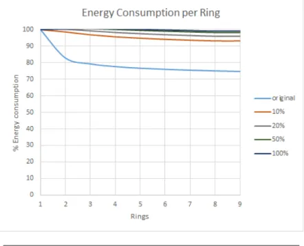
6.3 Energy consumption per ring for different values - Extended model . . . 47

6.4 Remaining Energy . . . 48

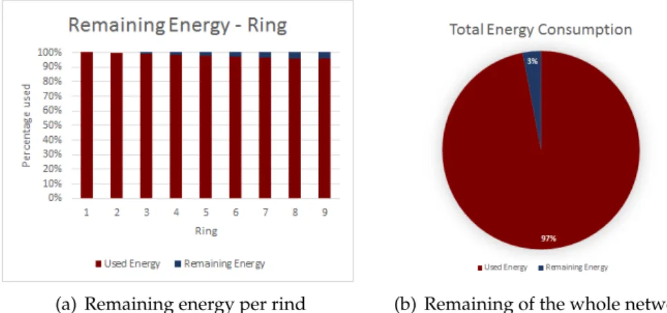
6.5 Distribution of energy consumption in each ring using relays 49 6.6 Energy consumption of the network using relay nodes . . . 50

(12)

(13)

xiii

List of Tables

3.1 Network Parameter Values . . . 12

3.2 Traffic Parameter Values . . . 14

3.3 Radio Model with Typical Parameter Values . . . 15

(14)

(15)

xv

To my parents, Juan and Socorro, my sisters Annel,

Anahi and Dianey who are always in my thoughts. . .

(16)

(17)

1

Chapter 1

Introduction

1.1 Wireless sensor networks

A typical wireless sensor network, shown in Fig. 6.7, consists of a large number of distributed detection stations called sensor nodes, with the abil-ity of recording and monitoring many different conditions such as temper-ature, humidity, pressure, wind direction and speed, illumination intensity, vibration intensity, sound intensity, power-line voltage, chemical concen-trations, pollutant levels and vital body functions.

These sensors are equipped with wireless interfaces with which they can communicate with one another to form a network. This self-organized infrastructure uses a multi-hop routing to deliver the collected information to some collection center commonly called sink.

FIGURE1.1: Typical Wireless Sensor Network.

Thanks to the rapid progresses in computer science, wireless commu-nication, Micro Electro Mechanical systems (MEMS) and Internet, the de-velopment of sensors that are smaller, cheaper, and intelligent has been possible, giving WSN the chance to use all their potential in many appli-cations. The design of a WSN depends significantly on the application, and it must consider factors such as the environment, the application’s design objectives, cost, hardware, and system constraints. Sensors in these kind

(18)

2 Chapter 1. Introduction

of applications are expected to be remotely deployed and to operate au-tonomously in unattended environments.

However sensor nodes in the network typically face severe computation and communication constraints but principally the energy depletion prob-lem. Its own nature of be a self-organized infrastructure that uses multi-hop routing to deliver the collected information to the sink, is its main disadvan-tage. In multihop wireless networks that are often characterized by many to one traffic patterns, it is very common to find problems related to energy depletion. Along the network, sensors experiment different traffic intensi-ties and energy depletion rates. Usually, the sensors near the sink tend to deplete their energy sooner because they act as data originators and data relayers and are required to forward a large amount of traffic of the most remote sensors to the sink while the sensors located in the periphery of the network remain much of the time inactive.

Sensors typically operate on batteries and are often deployed in harsh environment where human operators cannot access them easily, making it difficult or impossible to replace the batteries, that is why much of the re-search on wireless sensor networks has focused on the energy depletion in order to achieve energy efficiency to extend the network lifetime.

However, the challenge is not only reducing the power consumption of each sensor o increase the number of sensors near to the sink but also maintain a balance of energy consumption in the network, that is the key to prevent that certain nodes do not die much earlier than others, leading to unmonitored areas in the network.

So, maintaining a correct operation of the network is a fundamental ob-jective. However, the resource constrained nature of sensor nodes and the network, often propose non-conventional challenges and motivate the need for special techniques for the correct design and management of WSN.

1.2 Motivation

Energy consumption is a challenge in wireless sensor network applications because the energy of nodes is highly limited and difficult to be replenished and mainly because these applications need to operate for a long time. For example, habitat monitoring may require continuous operation for months, and monitoring civil structures requires an operational lifetime of several years.

The lifetime of a sensor network has several definitions in the literature. Some researchers consider the end of its lifetime when a node runs out en-ergy, in other words is the time when the system starts operation until the time when the first node exhausts its energy. Due to sensors nodes define the lifetime of the whole network, energy consumption has to be carefully balanced among them.

(19)

1.3. Goals 3 So, finding some distribution that allows a correct energy balance, is the main topic of this work.

1.3 Goals

In the field of WNS, more specific, in applications where the many to one traffic pattern is required, multihop forwarding may cause energy imbal-ance as all the traffic must be routed from the external nodes to the sink, creating a hot spot around the base station or commonly called sink.

Despite the fact that many node distribution strategies has been consid-ered in the literature, where the node density in regions closer to the sink is increased, in order to face the increasing traffic rate in those regions. There is no general framework to evaluate what is the best strategy that allow to achieve the maximum lifetime of the network. In other words, there is no easy way to compare the advantages and disadvantages of these various deployment strategies.

This work address the network energy balance problem and analyze the limits of network lifetime for different deployment distributions.

More specifically, this work proposes the deployment of extra relay nodes around the sink in order to solve the energy imbalanced problem. Through extensive simulations using different distributions the objective is to find an efficient way to adjust the density of relay nodes in order to guarantee that all nodes have balanced energy consumption and die almost at the same time.

(20)

(21)

5

Chapter 2

State of the art

In this chapter, we introduce the state of the art involving the most common challenges related to WSN with the objective to let the reader know a gen-eral idea of how this area has been evolved and to highlight the different efforts to solve these issues.

As we mentioned, several researchers have studied and addressed the most common challenges involved in the study of WSN. In this chapter we classified the related work into three categories: the energy hole problem, the node distribution strategies, this work mainly focus on it, and the en-ergy efficient design.

2.1 The energy hole problem

Various schemes have been proposed to address the energy hole problem. It has been shown analytically in [13] that the energy hole problem really exists in various sensor networks and in [15] the authors proved that the energy hole problem is inevitable under certain conditions. They also as-sume that the nodes are distributed uniformly in the network and report data constantly.

So, the energy hole is most common observed in networks where all the nodes are homogeneous and are deployed uniformly and need to send the data at constant rate to the sink. Since the entire network traffic flows toward the sink, the sensor nodes located in the periphery of the network need to send the sensing data to the sink. Due to the nature of the topol-ogy of the network, the traffic follows a many to one pattern, some sensor nodes far from the sink cannot send their data directly the sink and need other nodes to relay their data to the sink node. As a result, their energy consumption rates tend to be higher than those nodes that are far away from the sink because the nodes close the sink have to spend much energy to send their own data and relay the data sent by the far nodes, therefore, dying faster.

When the nodes close to the sink all die, no data can be sent to the sink and the sensor network stops working, leaving a hole near the sink and partitioning the whole network while many remaining nodes, commonly the nodes in the periphery, still have a plenty of energy Fig.2.1. This phe-nomenon is called the energy whole problem and when it appears no more data can be delivered to the sink. That phenomenon occur because sensor

(22)

6 Chapter 2. State of the art

networks often experience unbalanced traffic distribution which causes a considerable amount of energy is wasted, and the network lifetime ends prematurely.

FIGURE2.1: The energy hole problem.

Several studies have proved that when a node close to the sink runs out of energy, the remaining nodes have plenty of energy. Experimental results in [14] show that using a normal uniform deployment, up to 90 percent of the energy of the network can be left unused when the network lifetime is over. Likewise, in [15], the authors claimed that when the nodes one hop away from the sink use up all their energy, the remaining nodes have used only 7 percent of their energy on average.

2.2 The node distribution strategies

The main goal in sensor deployment is to determine the location of the sen-sor nodes that minimizes the cost, provides high coverage and resilience to failures, and notably prevent energy hole. Due to the multi-hop many to one traffic pattern typical in WSNs, the network often experiences un-balanced traffic distribution where sensor nodes act as data originators and relay nodes. In this case authors in [21] proved that an energy consumption rate is unavoidable if all the nodes in the network are homogeneous and are deployed uniformly in the network.

(23)

2.2. The node distribution strategies 7 In order to solve this issue, authors claim that by carefully increasing the number of nodes around the sink, they can prevent the sensor nodes near the sink from depleting their energy faster than others, and hence, resolve the energy hole problem. For example in [21] the author proved that com-pletely balanced energy consumption among all the nodes is impossible due to the own nature many-to-one traffic pattern in WSNs. Nevertheless, the balanced energy consumption in the network is still achievable but only if the number of nodes grows in geometric progression from the outer coro-nas to the inner ones except in the periphery of the network

Of course, adding more nodes to the areas with heavier traffic, espe-cially in the area closer to the sink, is a natural way to mitigate the en-ergy hole problem, also has other benefits, such as better connectivity and higher reliability, thus creating different node densities in different areas in the network. This is what is called non uniform node distribution. But the drawback of these solutions is that they considerably increase the number of nodes around the sink, which consequently increases the deployment cost. Therefore this solution is only effective in situations where inexpen-sive sensors can be mass-produced or in places where human operators can access them easily to add more nodes. Recent advances in micro-electro-mechanical and integration technologies make the first situation, cheaper nodes, more and more likely to occur.

Different studies using a non-uniform deployment have been presented in [21, 22, 23, 5, 1], where the node density in regions closer to the sink is increased progressively to deal with the increasing of traffic in those re-gions. The deployment of extra pure relay nodes around the sink can also be helpful in solving energy imbalanced problem [23,18].

FIGURE 2.2: Uniform distribution vs Non-uniform distri-bution.

(24)

2.3 The energy efficient design

Energy consumption is the bottleneck of wireless sensor networks because the energy of nodes is highly limited and difficult to be replenished for example a node is considered dead when it runs out energy. So energy con-sumption has to be carefully considered for sensor nodes.

The objective of energy management is to increase network operational lifetime through energy efficient protocols (Routing, MAC, etc.), for exam-ple, in [9], it show how energy consumption can be balanced by distributing packets over several paths.

To accomplish this goal of lifetime maximization, the load balancing us-ing a combination of intelligent routus-ing and transmission power control has been studied for many researchers; In [4], authors show how the optimal combination of several routing costs allows to extend the network lifetime, in [19] different heuristic routing costs were recommended for use in order to minimize and balance the energy consumption and the problem of find-ing the optimal routfind-ing path to achieve the maximum network lifetime in a sensor network was studied as a constrained linear program optimization in [2,17], and [24].

In [20] the energy hole problem is discussed, again, in WSNs with non uniform node distribution. They assume that the data rates of the nodes are tunable and only consider the energy dissipation in data transmission. The authors observed that balanced energy consumption is possible when the data rates are adjusted. The researchers in [21] study the same issue by adopting a more practical energy model that incorporates the energy spent in both data transmission and reception with the assumption that all the nodes constantly report data to the sink. They propose q-Switch Routing, a distributed shortest path routing algorithm adapted for the proposed non uniform node distribution strategy. It effectively switches the data flow among its corresponding next-hop forwarding candidates in order to bal-ance energy dissipation among them.

Other studies have addressed the energy consumption problem by care-fully placing more sink nodes over the network. In [1] authors claim that the location of the sink also can influence the network performance.

They opt to categorize the various strategies for statically positioning single and multiple sink in WSN, with the objective to help application de-signers identify alternative solutions and select appropriate strategies to determine the location of the sink.

In that work they highlight the potential of careful positioning of the sink and introduce dynamic schemes that reposition the sink during the network operation. They show that dynamic sink positioning can be very effective in optimizing the network functional and non-functional perfor-mance objectives in order to face dynamic changes in the environment and available network resources. In addition they argue that dynamically po-sitioning the sink while the network is operational can be a very effective

(25)

2.4. Mac Protocols 9 means for boosting the dependability attributes of the network. How ever since optimal sink positioning in WSN has proved to be NP-complete [8], several heuristics were proposed to find sub-optimal solutions [8,3,16].

The deployment of extra relay nodes around the data sink can also be helpful in solving energy imbalance problems. In [6], autors define the relay nodes as simple energy deposits. In their work, they present the optimal en-ergy distribution map for the network which is used to determine the areas where energy is insufficient and thus determine where relay nodes should be placed and how much energy they should carry.

In [10], authors compare the minimum energy consumption when the relay nodes’ locations are predetermined and when they can be placed in any location. The authors provide a heuristic method to solve this prob-lem. In [11], a similar mixed-integer nonlinear programming solution is provided to discover the optimal locations of relay nodes iteratively.

2.4 Mac Protocols

Another important issue in the study of Wireless Sensor Networks (WSNs), are the MAC protocols, which arose from the requirement to achieve an effi-cient consumption of energy within the network. Some application scenar-ios for Wireless Sensor Networks (WSNs) often involve battery-powered nodes being active for considerable lengths of time, several months to years, without external control by human operators after initial deployment. Since the batteries have a limited capacity of energy, the use of these without any type of energy strategy can cause that a node will deplete its batteries within a couple of days. This fundamental need for energy-efficient op-eration has drawn the attention to the radio, which is the component of a typical sensor node that consumes most energy.

Energy saving is achieved at the MAC protocol by duty-cycling the ra-dio, that is, repeatedly switching it between active and sleep modes. This is the only way to achieve the required two orders of magnitude reduction in energy consumption for extending lifetime from days to years. This duty cycling effectively reduces the available bandwidth on the radio channel, and hence limits the amount of data that can be communicated through the sensor network.

In active mode, a node can receive and transmit packets, while in the sleep mode, it completely turns off its radio to save energy. However, for-warding a packet over multiple hops in duty-cycled MAC protocols often requires multiple operational cycles, where nodes have to wait for the next cycle to forward data at each hop.

In [7] authors investigate the inherent trade-off between energy con-sumption and e2e delay from a game theory perspective applied to six Wireless Sensor Network (WSN) MAC protocols; B-MAC, X-MAC, RI-MAC, SMAC, DMAC, and LMAC. In this work the two optimization objectives (energy consumption and e2e delay) are considered as game players. The

(26)

cost model of each player is mapped through a generalized optimization framework onto protocol specific MAC parameters. From the optimiza-tion framework, a game is first defined by the Nash Bargaining Soluoptimiza-tion (NBS) to assure energy-consumption and e2e delay balancing. Secondly, the Kalai-Smorodinsky Bargaining Solution (KSBS) is used to find equal proportion of gain between players. The result shows the effectiveness and scalability of such framework in optimizing protocol parameters that achieve a fair energy-delay performance trade-off under the application re-quirements.

In [12] the author shows a study of the different MAC protocols in the literature. In his work he mentions that these protocols differ in how per-formance (latency, throughput) is traded off for a reduction in energy con-sumption. He also mentioned that the performance of each protocol de-pends on specific details of the application. In that work, he seeks to dis-cover which is the best protocol for low data-rate applications where colli-sions are of little concern, making an analytical approach tractable in which latency and energy consumption are modeled as functions of key protocol parameters (duty cycle, slot length, number of slots, etc.).

These MAC protocols all trade off performance (latency, throughput) for a reduction in energy, but differ in complexity and flexibility to adapt to traffic fluctuations, topology changes, and varying channel conditions. That’s why developers of long-running applications must be careful in se-lecting the MAC protocol that suits their needs best, so that they can squeeze the most out of the limited hardware resources.

(27)

11

Chapter 3

Models and equations

In this chapter we proceed to describe in detail the network and traffic model used in this simulation, the main features of the radio device, the X-MAC protocol and of course the system energy used to present our find-ings.

3.1 Network model

For a sake of simplicity, a ring topology is used, although this modeling can be easily adapted to other network topologies, e.g. random topology or grid topology.

FIGURE3.1: Spanning tree

A spanning tree is constructed Fig.3.1, where nodes are static and maintain a unique path to the sink and use the shortest path routing with a maximum length of D hops; the depth or num-ber of rings of the tree. We as-sume a network with size of N nodes, a uniform node density on the plane and a unit disk graph communication model.

There areC+ 1nodes, in average, on the unit disk. Hence, all nodes are in communication range with an average number of neighbors,C, except the leaf nodes. The nodes are layered into levels according to their distance to the sink in terms of minimal hop count, d(d = 1, ..., D), where d= 0 is reserved for the sink.

Taking the idea explained above, in Fig.3.2, we can see an example of the topology used in this study. As we can observe a ring topology is shown with a depth ofD = 3. In the inner ring,D= 0, we can find the sink node in which all network traffic is concentrated. The nodes located at the fol-lowing rings has on averageC = 2neighbors nodes except the nodes that are in the last ring. Thus using the formulaN = (2d−1)C, which will be explained shortly, the total number of nodes in the network is obtained.

All values used in this study, involving the network model are summa-rized in Table3.1.

(28)

12 Chapter 3. Models and equations

FIGURE3.2: Sample of a ring topology,C = 2,D = 3and

N = 18.

Network Parameter Description Values

N Network Size (number of nodes) [nodes] 200-512

D Network Depth [levels] 5-9

C Network Density (Connectivity) [neighbors] 4-8

TABLE3.1: Network Parameter Values

3.2 Traffic model

For this work, we have used the traffic model used by Langendoen [12], we consider an unsaturated network topology with periodic traffic generation, which is typical of WSN applications.

In our model every source node generates traffic with frequency FS. According to this, we will use in our modeling the terms; inputF_ind, output F_outd , backgroundF_Bd traffic andIdfor the input links.

The neighboring nodes, then, can be classified as the set of children (in-put) nodes I and the set of overheard (background) nodes, B, such that, C=|I|+|B|.

Using the previous topology mentioned, let us define the following pa-rameters;

Ndis the number of nodes in ringd: Nd=

1, ifd= 0,

(29)

3.2. Traffic model 13

The average number of input linksIat node at leveldis:

|Id|=    0, ifd=D, C, ifd= 0, Nd+1 Nd = 2d+1 2d−1, otherwise, (3.2)

whereDdenotes the maximum distance to the sink. Assuming a sam-pling rate ofFS, the output frequency defined as the number of packets that leaves a node is:

F_outd = ( FS, ifd=D, F_ind +FS =|Id|Foutd+1+FS =FS(D 2₋_d2₊₂_d₋₁₎ (2d−1) , otherwise. (3.3)

and thus the input frequency,F_ind, defined as the number of packets that enter a node is:

F_ind = ( FSD2C, ifd= 0, |Id|Foutd+1=FS(D 2₋_d2₎ (2d−1) , otherwise. (3.4)

Finally, the aggregated background traffic frequency is:

F_Bd =|Bd|Foutd = (C− |Id|)Fout (3.5)

whereBdis the average number of background nodes.

Taking the idea explained above, the network traffic does not necessar-ily can begin from the farthest nodes, but also the nodes located on the inner rings have the ability to generate traffic.

As we can see in Fig.3.3, all network nodes can generate their own traf-fic and send it to the inner rings. Each node in the inner rings are able to generate its own traffic and also are responsible for receiving the traffic from the upper nodes and forward it to the lower nodes in order to reach the sink node.

As shown in Fig.3.3, the closer to the sink, there will be more traffic, so that, the nodes located in the lower rings are more active causing that their wear be greater than the nodes located at the periphery of the network.

(30)

All values used in this study, involving the traffic model are summa-rized in Table3.2.

FIGURE 3.3: The traffic flows from the upper levels until reach the sink node.

Traffic Parameter Description Values

P Data payload [byte] 32

FS Sampling rate [pkt/node/min] 0.01−15

F_Id Node’s Input Traffic Frequency at leveld F_outd F_outd Node’s Output Traffic Frequency at leveld FS Fd

B Background Node’s Traffic Frequency at leveld background

TABLE3.2: Traffic Parameter Values

3.3 Radio model

Besides the network model and traffic parameters, the evaluation of a MAC model requires information about the radio hardware that will be used, in order to build the system energy and delay model.

For this part the main parameters of a radio to consider are: the time needed to power it up (i.e.,to transit from sleep into active mode), its data rate, and the time needed to do a carrier sense (including power-up), and of course the amount of energy consumed in its different states (i.e. Energy consumption in Sleep state ).

(31)

3.4. MAC protocol Model 15

FIGURE3.4: CC2420 Radio

In our simulation we used the CC2420 radio, Fig. 3.4, a true single-chip 2.4 GHz IEEE 802.15.4 compliant RF transceiver de-signed for low power and low voltage wireless applications. It includes a digital direct sequence spread spectrum baseband modem providing a spreading gain of 9 dB and an effective data rate of 250 kbps.

The CC2420 is a low-cost, highly integrated solution for robust wireless communication in the 2.4 GHz unlicensed ISM band and provides extensive hardware support for packet handling, data buffering, burst transmissions, data encryption, data authentication, clear channel assessment, link quality indication and packet timing information. These features reduce the load on the host controller and allow CC2420 to interface low-cost microcon-trollers.

All values used in this study, involving the radio model are summarized in Table3.3.

CC2420 Radio Parameter Description Values

R Rate [kbyte/s] 31.25

Tcs Time [ms] to turn the radio on and probe the channel 2.60

Tup Time [ms] to turn the radio on into RX or TX 2.40

Lpbl Packet preamble length [byte] 4

Rx Energy consumption in Rx state [mA] 19.7

T x Energy consumption in Tx state [mA] 17.4

Cs Energy consumption in Carrier Sense state [µA] 426

Sleep Energy consumption in Sleep state [µA] 20

TABLE3.3: Radio Model with Typical Parameter Values

3.4 MAC protocol Model

The energy efficiency problem seen in WSN has produced many different specialized medium access control (MAC) protocols. The main contribu-tion of these protocols is the duty cycling the radio that achieves the energy saving by repeatedly switching the radio between active and sleep modes. For this work we choose the duty-cycle XMAC protocol.

X-MAC is an asynchronous preamble sampling based protocol where nodes wake up periodically every Tw seconds to perform carrier sensing for,Tcs+Tal, (1).To send a packet, a node first contends to access the chan-nel within the contention windowTcw, and it transmits a sequence of strobe preambles of durationTps, which are short packets containing the identifier of the receiver. It then listens to an acknowledgment for Tal (2). Strobes continue for a period sufficient to make at least one strobe overlap with a receiver wake-up (3). The receiver replies with an acknowledgment of du-rationTack(4) and keeps the radio on. After that, the sender transmits the

(32)

FIGURE3.5: X-MAC’s carrier sensing, transmission, and re-ceiving modes.

data packet,Tdata, which spans for the transmission of the header and the payload (5).

The main adjustable parameter that affects the energy and delay perfor-mance is mainly the wake-up period,Tw, and hence the vector parameter for X-MAC protocol is given byXXM AC = [Tw].

All values used in this study, involving the XMAC Protocol are summa-rized in Table3.4.

X-MAC Parameter Description Values

Tw Wake-up Period [ms] 100−400

Lpbl Preamble length [byte] 4

Lhdr Header length [byte] 9 +Lpbl

Lack ACK length [byte] 9 +Lpbl

Lps Preamble strobe length [byte] 5 +Lpbl

Tal Ack listen period [ms] 0.95

Thdr Header transmission duration [ms] Lhdr/R; Tack ACK transmission duration [ms] Lack/R; Tps Preamble strobe transmission duration [mA] Lps/R

Tcw Contention window size [ms] 15∗0.62

Tcs Time [ms] to turn the radio into TX and probe the channel 2.60

Tdata Data packet transmission duration [ms] Thdr+P/R+Tack

TABLE3.4: Values for X-MAC setting

3.5 System energy model

The energy consumption of nodeEn, based on the protocol operation modes, is defined as the amount of energy consumed by the radio duty of the node in the network according to its location and the amount of traffic it handles. Hence, the energy consumption of the node is the sum of energy consumed in each operating mode, which depends on the exchanged traffic load and the XMAC intrinsic parameters.

(33)

3.6. Delay model 17 In general, for any MAC protocol in the literature, the node’s consumed energy is caused by carrier sensingEcs, data transmissionEtx, data receiv-ingErx, overhearingEovr, and by sending/receiving explicit synchroniza-tion, respectively denoted byEstxandEsrx.

For example, letE_csn, E_txn,E_rxn andE_sleepn be the energy consumed frac-tions for nodenin idle listening, transmitting, receiving, and sleeping modes respectively.

The normalized energy consumption (in Amperes) can be calculated by multiplying the obtained expressions in each mode by the values of the ra-dio consumption mode defined in the Table3.3.

The energy consumption of the node can be calculated as:

En=E_csn +E_txn +E_rxn +E_ovrn +E_sleepn (3.6) where E_csn = (Tcs+Tal) Tw (3.7) E_txn = (Tcs+Tal+Ttx)Foutn (3.8) E_rxn = (3 2Tps+Tack+Tdata)F n in (3.9) E_ovrn = (3 2 Ttx Tw Tps)F_Bn (3.10) E_sleepn =Tw−(Ecsn +Etxn +Erxn +Eovrn ) (3.11) and Ttx= ( Tw Tps+Tal )Tps+Tal 2 +Tack+Tdata (3.12) While the maximum energy consumption in the whole network is:

E = N X n=1 (E_csn +E_txn +E_rxn +E_ovrn +E_sleepn ) (3.13)

3.6 Delay model

The end-to-end (e2e) packet delay (latency), Ln, is defined as the expected time between the first transmission of a packet at node,n ∈ N, and its re-ception at the sink.

It is then a per-topology parameter, in the sense that it depends on the position of the node that generates the data. Lndenotes the sum of per-hop latencies of the shortest path,Pn, from nodento the sink, whereLn_l is the

(34)

one-hop latency on each linkl∈Pn.

The end-to-end latency of nodenat leveldn_is:

Ln_dn = dn X i=1 (Tw 2 + Tcw 2 +Tdata) (3.14) where Tdata=Thdr+ P R +Tack (3.15)

3.7 The bottleneck constraint

The bottleneck is at the sink node, which has to receive all (data and sync) messages injected into the network. In order to avoid hidden terminal col-lisions at the sink, there should only be one message every fourth slot.

The bottleneck constraint:

I0 E1_tx< 1 4 (3.16) whereI0

(35)

19

Chapter 4

Dutycycle MAC protocols

-Energy conservation

In this chapter we define the parameters of our baseline study before start-ing our research proposal in the deployment of extra relay nodes.

Basically we start defining our network topology for this study. Then based on this structure we study the behavior of the delay and energy when it is subject to certain restrictions that we have defined for this job, in order to find the best values that enable optimal latency and energy consumption. And finally using these values, the Nash Bargaining scheme is used to find the tradeoff between energy conservation and latency that gives us the best energy gain for these restrictions.

In other words, the objective of this project is to optimize a duty-cycle MAC protocol in order to minimize energy consumption and e2e delay and show that even using these tools still exist a significant percentage that can be further reduced thus ensuring additional savings and even increase the lifetime of the network. With this idea, we justify our proposal to add ad-ditional relay nodes in order to find an efficient way to balance energy.

For this part we have used the proposed equations and models used in [7].

4.1 X-Mac Protocol Analysis

The exact behavior of the MAC models depends on the settings of some protocol specific parameters. In this case the performance of XMAC strongly depends on the main adjustable parameter that affects the energy and delay performance is mainly the wake up period,T w.

Besides of the wake up period, the optimal settings of the X-MAC pro-tocol parameters depend on other external conditions like the traffic rate Fs, the network model and the radio characteristics.

In the analysis presented in this section we set the wake up period and the sampling rate in the intervalTw∈[100,40][ms]andFs∈[1,15][pkt/node/min] respectively and for the network and radio, we used the parameters previ-ously defined in Table3.3. For these settings we compute the performance metrics of interest, for example, latency and energy efficiency.

(36)

20 Chapter 4. Duty-cycle MAC protocols - Energy conservation

The equations used to calculate the energy consumption are:

EXM AC = max n∈N( α1 Tw +α2Tw+α3) (4.1) where α1=Tcs+Tal+ 3 2Tps( Tps+Tal 2 +Tack+Tdata)F dn B (4.2) α2 = F_outdn 2 (4.3) α3 = ( Tps+Tal

2 +Tcs+Tal+Tack+Tdata)F dn out+( 3 2Tps+Tack+Tdata)F dn in + 3 4TpsF dn B (4.4)

The equations used to calculate the e2e delay of the network are:

LXM AC = max n∈N(β1Tw+β2) (4.5) β1= dn X i=1 1 2 (4.6) β2= dn X i=1 (Tcw 2 +Tdata) (4.7) 4.1.1 Energy consumption

The energy consumption (duty cycle) of XMAC depends on the main ad-justable parameter that affects the energy performance is mainly the wake up period, Tw. In XMAC the nodes are required to perform a (synchro-nized) carrier sense in every slot each wake-up periodTw to check for a potential message.

Setting the network topology ind= 9,c = 4, resulting in a total of 324 nodes, in Fig.4.1we can see that the number of packets sent every half hour Fshas a significant impact on energy consumption. Observing the energy consumption as a function of different frequencies, we can see that it clearly has two different behaviors, one behavior for small frequencies and one be-havior for large frequencies.

In the case of setting a small frequency, we can see that asTw becomes larger the energy tends to decrease. In the case of setting a large frequency, we can see how energy descends and starts to rise rapidly. For this case we can see that a large value ofTwincreases the energy consumption. This is because when the protocol is forced to spend more time in sleep state, when a node wants to send a packet, it will spent more time in statex send-ing bicons for a longer time until the other node wakes up and receives its

(37)

4.1. X-Mac Protocol Analysis 21

FIGURE4.1: Energy consumption for different values ofFs.

packet and so on for the other nodes, which makes consumption increase. In other words, when we increase the frequency of packets, it results in a progressive power consumption. Taking into consideration the behaviour of Tw, we note that when the amount of traffic increases a larger wake-up period is needed.

(a) Case 1: Low frequencyFs (b) Case 2: High frequencyFs

FIGURE4.2: Behavior of energy consumption as a function of different frequencies ofFs.

By studying the two extreme cases seen in Fig.4.2, setting a high traffic rate (15 packages every half hour), it is shown that energy tends to increase while in the other hand using a small traffic rate (0,5 packages every half hour) the energy consumption tends to decrease. With that analysis we can see that this kind of protocol is ideal in scenarios where a high packet traffic is not required, maintaining a small power consumption.

4.1.2 Delay

In XMAC the delay is translate as the minimum amount of time between message and message. This means that by having a small wake-up period

(38)

Tw, the protocol becomes more active, since the waiting time is reduced more packets are sending per time unit. On the other hand by defining a long wake-up period, the amount of time between each message will be higher resulting in a low activity inside the protocol.

As we can see in Equation 4.5 and Fig.4.3, the latency of XMAC has a linear behavior, always depending onTw. Also can be seen that the fre-quency has no impact on the behavior of the delay so this remains constant for different values of traffic rateFs.

FIGURE4.3: e2e Packet Delay for different values ofFs.

4.1.3 Latency vs Energy

Analyzing the calculated values of energy consumption and the e2e delay seen in Fig.4.1and Fig.4.3for different values ofFs, whereFsdepends on the wake-up periodTw, we can see clearly a correlation between the energy consumption and the e2e delay.

In Fig.4.4, it can be observed that when the objective is to reduce the e2e delay, it causes a rising of energy consumption while to maintain a low power consumption is achieved at the cost of high latency.

Now we know how the length of the wake-up period,Tw has impact in the behavior of the e2e latency and energy separately, and how this period creates a correlation between both of them, the next step is optimize theTw parameter.

So the objective is to obtain the optimal value for the tuning parameter Tw that minimizes energy consumption and e2e delay in a fair manner.

(39)

4.2. X-Mac Protocol Optimization 23

FIGURE4.4: e2e Delay vs. Energy for different values ofFs.

4.2 X-Mac Protocol Optimization

So far we have located and identified three possible scenarios for optimiz-ing the wake-up timeTw. The first scenario would be for applications where the delay is not a problem and is required an optimal energy consumption. The second scenario would be for applications where energy consumption is not a problem and is required a specified delay.

For the third one scenario would be where a balance is sought between energy consumption and e2e delay that is to say find the optimal value for wake-up valueTw that minimizes energy consumption and e2e delay in a fair manner.

In order to find the optimal trade-off solution for scenario one and sce-nario two, we define a bargaining problem in which each optimization problem represents a player, i.e., player Energy and player Latency. The Bargaining problem is a problem of understanding how several agents should cooperate when non-cooperation leads to Pareto-inefficient results. The so-lution of the problem is one that coincides to the soso-lution that an arbitrator would recommend. In order to solve this problem the Nash Bargaining So-lution (NBS) is used.

For the first scenario we will use the optimization problem (P1), for the second the optimization problem (P2)and for the last one the Nash Bargaining scheme(N BS).

4.2.1 Energy Optimization for Duty-Cycled MAC

Since we want to optimize energy consumption, we take the worst case conditions. Due to the nature of our network, we know that the most traffic rate is located in the nodes closest to the sink, more specifically the nodes located in the ring number one,d= 1, so we take this value as the biggest energy consumption that a node can have. That means, that related to equa-tions in chapter 3, in the energy equaequa-tions, F_outdn, F_indn and F_Bdn have to be

(40)

accorded todn= 1.

Given the application requirements in terms of e2e packet delay bound Lmax, energy optimization derives optimal MAC parameters that give the minimal network energy consumption subject toLmax:

(P1) M inimize EXM AC(Tw) s.t. LXM AC(Tw)≤Lmax Tw≥Twmin (4.8) I0 E_tx1 < 1₄ V ar. Tw

whereLmaxis the maximum latency tolerated by the application. In Fig.4.5, we show the results of our tests for the optimization of en-ergy subject to delay. For this we have defined an intervalLmax∈[0.15][S] that we have used to solve our optimization problem (P1). As in the previ-ous simulations the values have been set atd= 9,c= 4. Once defined our topology we set different frequencies and in each one, we tested different values ofLmaxto locate the different optimum points.

FIGURE4.5: Energy consumption subject to several values of Latency

In the figure mentioned we can see different minimum points for differ-ent frequencies. As we mdiffer-entioned before there are two differdiffer-ent behaviors, one where energy tends to decrease and another where it decreases and rises sharply. In the simulations with a low traffic frequency, in the interval Lmax, it shows that for values between 0.1 and 5 seconds it is possible to find different optimal points that satisfy our maximum latency condition. While for applications that requires a higher frequency, case 2, we observe that as traffic increases, it can be noticed how the optimum point begins to converge towards a single point. For example in Fig.4.6case:f, it does not matter the value ofLmax, in the interval [0.1, 5], the result will always give

(41)

4.2. X-Mac Protocol Optimization 25 the same optimum point. Which is obvious since we are facing the global minimum of our energy consumption.

(a)Fs= 0.1 (b) Fs= 0.5

(c)Fs= 1 (d) Fs= 5

(e) Fs= 10 (f) Fs= 15

FIGURE 4.6: Behavior for Minimum energy consumption

for several values ofFssubject to different values of delay,

(42)

4.2.2 Delay Optization for Duty-Cycled MAC

Since we want to optimize the delay, we take the worst case conditions. Due to the nature of our network, we know that the maximum delay allowed in the network is from the nodes located in the periphery of the network, d=D. That means, that related to equations in chapter 3, the delay equa-tions3.14have to be accorded todn=D.

Given the application requirements in terms of maximum energy bud-getEbudgetexpressed as the maximum allowed duty cycle, we are interested in finding the optimal MAC parameters that give the minimum e2e packet delay subject to maximum energy budget:

(P2) M inimize LXM AC(Tw) s.t. EXM AC(Tw)≤Ebudget Tw≥Twmin (4.9) I0 E_tx1 < 1₄ V ar. Tw

whereEbudget is the energy budget (maximum duty cycle) that a node consumption cannot exceed for fulfilling a lifetime target.

FIGURE 4.7: Latency subject to several values of Energy consumption (Ebudget)

As we already mentioned before the traffic rate Fs has no positive or negative impact on the delay so always it remains constant for different values ofFs.

Even using different values ofEbudget for solve the optimization prob-lem (P2), the solution is always the same. By having a linear behavior, it can be seen perfectly in Fig.4.7which is its lowest point for all values ofFs. Also the selected values for Maximal EnergyEbudge ∈[0.5,5]not present a significant value hence you always will obtain a minimum point508,554[s] forTw= 100 for all different values ofEbudgetandFs.

(43)

4.2. X-Mac Protocol Optimization 27 4.2.3 The Nash Bargaining Solution (NBS) for Duty-Cycled MAC The Nash bargaining solution, Fig.4.8is a simple two-player game used to model bargaining interactions. In the Nash bargaining game, two players demand a portion of some good, in this work our players are Energy and Latency and they are demanding some time (Wake-up timeTw) in order to decide how much energy will be used in sending and receiving messages (Duty cycle) and how much time the protocol have to wait between mes-sage and mesmes-sage. If the total amount requested by the players is less than that available, both players get their request. If their total request is greater than that available, neither player gets their request. A Nash bargaining solution is a Pareto efficient solution to a Nash bargaining game.

FIGURE 4.8: The Nash Bargaining Solution (NBS). The so-lution (E∗, L∗) of the optimization problem (NBS) where

E∗ =E(X∗)andL∗ = L(X∗)will be the optimal cost for both players under the agreement.

In this game, let intervalsAE = [Eworst, Ebest]andAL = [Lworst, Lbest] be the set of strategies that respectively player energy and player delay may take, andsE ∈AE,sL∈AEthe strategies chosen by the players. The threat strategy for player delay is to play strategy, Lbest, that makes the player energy to get,Eworst. On the other hand, the threat strategy for player en-ergy is to play strategy, Ebest, that makes the player delay to get, Lworst. Let vE = Eworst, and vL = Lworst, be the threat values of each player, where each threat value represents the utility threshold of each player to sign the agreement. If no feasible solution is found, each player gets a cost φ(S;v) =∞. Note thatE(X)andL(X)are cost functions instead of utility functions, i.e., signs have to be reversed, and the term(E(X), L(X)) ∈ S represents the intrinsic conditions that each MAC protocol has to fulfil. The (NBS) problem is expressed as:

(44)

(N BS) max (Eworst−E(Tw))(Lworst−L(Tw)) s.t. (Ebudget, Lmax)≥E(Tw), L(Tw)

(Eworst, Lworst)≥E(Tw), L(Tw) (4.10) E(Tw), L(Tw)∈S

V ar. Tw

where theE(Tw), L(Tw) ∈ S means that we have to include the MAC protocol intrinsic conditions and where the point(Eworst, Lworst)is the dis-agreement point. The problem (NBS) is non-linear non-convex, but this kind of problems can be transformed into a standard convex optimization problem without changing its solution. The idea is to define auxiliary vari-ablesE1 andL1 such thatE1 ≥ E(Tw) andL1 ≥ L(Tw), which should be satisfied by the optimal solution. Wheneverthe problem (NBS) is feasible, E(Tw) ≤ Eworst, L(Tw) ≤ Lworst, and application of (NBS) to the MAC protocols yields a concave problem.

(N BS∗) max log(Eworst−E1) + log(Lworst−L1)

s.t. (Eworst, Lworst)≥(E(Tw), L(Tw))

(E1, L1)≥(E(Tw), L(Tw)) (4.11)

(E1, L1)≤(Ebudget, Lmax) (E1, L1)∈S

V ar. E1, L1, Tw

Consequently, the equivalent concave problem for XMAC is:

(N BS−XM AC∗) max log(E_worstXM AC −E1) + log(LXM ACworst −L1)

s.t. E_worstXM AC ≥EXM AC(Tw) E1 ≥EXM AC(Tw) LXM AC worst ≥LXM AC(Tw) (4.12) L1 ≥LXM AC(Tw) Tw ≥Twmin I0 E_tx1 < 1₄ V ar. E1, L1, Tw

(45)

4.2. X-Mac Protocol Optimization 29 4.2.4 Trade-Off Energy vs Latency

As we mention before the objective of use the NBS is to obtain the opti-mal valueTw that minimizes energy consumption and e2e delay in a fair manner. For analyzing this trade-off, the optimization problems (P1) and (P2) were solved first in order to determine the best values that permit to achieve optimal energy and delay objectives.

The image below shows the results of calculating different equilibria points. As we have already commented, we have detected different behav-iors as we have varied the frequency. Fig.4.9(a) shows the best equilibria points when we have a low frequencyFs. As we can see, when we have a low frequency it is more likely that different combinations of latency and energy constraints (e.g. setting a delay value and varying it with different energy values or vice versa) produce different equilibrium points. While in the presence of high frequencies the combination of these restrictions pro-duce a series of very close points between them that show a tendency to converge in a single point Fig.4.9(d).

(a)Fs= 0.5 (b) Fs= 5

(c)Fs= 10 (d)Fs= 15

FIGURE 4.9: Different equilibria points subject to several values ofLmax∈[0.1,5]andEbudget∈[0.1,5]

Analyzing these results we have noticed that the frequency affects the efficiency of the duty cycle. As shown in Fig.4.2, where both a very short and a very long sampling period will result in a high duty cycle (i.e., low efficiency), but their causes differ. While a short polling period will increase

(46)

the energy consumption for idle listening, a long one will increase the en-ergy consumption for transceiving the wakeup preamble. This has led us to study, how these constraints behave when frequency increases, at the time of calculating our optimalTw.

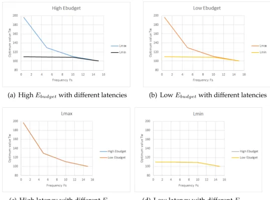
Fig.4.10shows the behavior ofTwwith respect to different frequencies using different combinations of constraints. In the mentioned figure we have summarized four different scenarios. In Fig.4.10(a) we have a high value ofEbutget (i.e. 5[mA]) where we have varied the delayLmax(from 5 to 0.6 seconds). In Fig.4.10(b) we have a low value ofEbudget(i.e. 0.1[mA]) and we have varied the latencyLmax. In Fig.4.10(c) we have set a high de-layLmax(i.e. 5 seconds) value and we have varied the energyEbudget. And finally in Fig.4.10(d) we have set a small delay value and we have varied the energy.

For example, Fig.4.10(a) a shows the behavior of our optimalTw when we set a high Ebudget (for example 5 [mA]) and use high and low delay values,Lmax andLminrespectively. In this case it is seen that using a very large delay, the value ofTwtends to fall very fast to compensate for a longer wait time, whereas when we use a small delay the value ofTwtends to be more stable. According to our results we have noticed that when setting an energy value no matter if it is high or low, the delay has a great impact on Tw Fig.4.10(a) and Fig.4.10(b). While fixing a latency value and subjecting it to different energy values, it does not affect the behavior of tw at all, Fig. 4.10(c) and Fig. 4.10(d). In other words, between delay and energy, delay is the most influential factor in the energy consumption of a wireless sensor networks.

(a) HighEbudgetwith different latencies (b) LowEbudgetwith different latencies

(c) High latency with differentEbudget (d) Low latency with differentEbudget

FIGURE 4.10: Trend of optimumTw for several values of

(47)

31

Chapter 5

Adding extra relay nodes

In this chapter, we propose a modification to the original model proposed by Langendoen [12], which allows the addition of extra nodes of relay class, in other words nodes that do not generate any type of data and only direct the existing traffic towards the sink, with the objective of reducing the en-ergy consumption in the internal rings distributing the traffic with the help of these new nodes.

5.1 Why Add extra relay nodes?

In order to achieve equal power consumption at different levels of our net-work, we have decided to add extra relay nodes to reduce and balance the traffic load that normal nodes have to carry. As mentioned above, each level within the network faces a different amount of traffic, which becomes more intense as we approach the interior levels. This behavior causes that the external nodes, with less traffic to handle, stay more time at rest while the nodes in the inner rings face a great amount of traffic which forces them to be more active, generating a more accelerated exhaustion, reason why nodes located in the inner rings exhaust its battery faster causing the life-time of the network to come to an end.

While the nodes located in the inner rings have died, the nodes in the outer rings still retain much of their energy, which tells us that the network has not yet reached its full potential.

In order to maintain a better balance we have added anN r number of relay nodes to a common implementation (original model, [12]). Knowing that the greatest wear is generated in the internal nodes, our logic tells us that adding a greater number of relay nodes in the inner rings would re-duce their wear therefore we could extend the lifetime of the network.

The how and where the new relay nodes are added is defined by a se-ries of distributions that we have chosen for our work. The key to choosing our deployment strategy has been the natural form of linear, quadratic, and exponential functions. For example, following our analysis of attacking the problem of energy distribution in the inner rings by adding extra relay nodes, the exponential distribution fits our problem, since the shape of this distribution, suggests us to add a large number of relay nodes in the inner rings and as it continues to add fewer nodes in the outer rings. Similarly following a linear distribution it is proposed to add a numberN rrelays in

(48)

32 Chapter 5. Adding extra relay nodes

the inner rings and gradually decrease the quantity until reaching the last ring. We also study the wear of all nodes when we add the same number of relays per ring (uniform distribution).

All these simulations have been done with the objective of finding the best distribution that best fits our problem, achieving a better energy distri-bution.

5.2 New traffic model

FIGURE5.1: New traffic model For deriving the new traffic model,

we extend the one proposed by Langendoen [12], for a homoge-neous sampling rate sensor net-work to a model for a multi-class sampling rate sensor network in which we have two classes of nodes, nodes of normal class and nodes of relay class, where each class has its own sampling rate. For each node of normal class letFs be

the rate at which it samples the environment, andFrbe the sampling rate or each node of relay class. The purpose of the modification of the traffic model is to add extra relay nodes that do not generate traffic, so for the study of this work we setF r= 0.

Just like the original model seen in chapter 2, we have:

T otalN odes=N n+N r (5.1)

WhereN nrepresents the total number of nodes of normal class.

N n=C∗D2 (5.2)

andN r represents the total number of nodes of relay class that will be added to the network.

N r =C∗D2∗αR (5.3)

whereαRis the percentage of extra relay nodes added in the network. The nodes are grouped into rings according to their distance to the sink. The first ring containsCnodes, from which we can derive the node density in each ring.

The average number of nodes of normal classNdin ringdis,

Nd= (2d−1)C (5.4)

and the average number of nodes of relay class in ringdisRd. HowRd is calculated, is shown in the following section.

(49)

5.3. Deployment distributions 33

5.3 Deployment distributions

As we discussed a moment ago the deployment of the number of relaysRd in the ringddepends on the distribution that is being used.

In this section different deployment strategies are proposed, maintain-ing the common goal of addmaintain-ing a greater number of relays nodes in the inner rings, where they are necessary because of the high amount of traffic and fewer relay nodes in the external rings where they are not so necessary. In other words the deployment strategy will follow a tendency to progres-sively add a numberN rof relay nodes from the periphery of the network to the inner rings.

To study and compare the impact of adding this type of nodes we pro-pose four different deployment strategies, based on their natural increase; uniform, linear, quadratic and exponential.

5.3.1 Uniform distribution

Since the objective is to study the effect of different strategies, we have started using the simplest and most common one by placing a N r num-ber of relay nodes in an equal proportion on all the rings in our network except in the last one.

First, we define the number of relay nodes that will be added to each ring, in this case being a uniform distribution, we add the same number of relay nodes to each ring except the last one. The purpose of these re-lay nodes is to direct and reduce the traffic without generating any type of data, so having this type of nodes in the last ring is useless Fig. 5.2, so we distribute the number of relay nodes that will be aggregated betweenD−1 rings.

Rd= N r

D−1 (5.5)

(a) Uniform Deployment (b) Uniform Distribution

(50)

5.3.2 Linear distribution

For this strategy we have chosen two behaviors, when it has a positive slope and when its slope is negative, Fig.5.3. We use the positive behavior to add the relay nodes starting from the ring d = 1 increasing its population lin-early until reaching the periphery, fewer nodes in the center, more nodes in the periphery. On the other hand we use negative behavior, starting from the periphery and continue to add relays in a linear way as we approach the center, more nodes in the center, fewer nodes in the periphery.

(a) Fewer in the center, more in the periphery

(b) More in the center, fewer in the periphery

FIGURE5.3: Linear deployment strategy

The original idea is to add a large number of relay nodes in the rings where there is more data traffic and where the population of nodes is small which causes its saturation and an early death. But we also want to know what happens when we map more nodes to the outer rings and less to the inside of the network. That is why, using this strategy, more nodes in the center fewer nodes in the periphery or fewer nodes in the center more nodes in the periphery, will help us locate where these new nodes really are needed.

(a) Linear Deployment (b) Linear Distribution

FIGURE5.4: Example of a linear deployment following the strategy, more nodes in the center fewer nodes in the

(51)

5.3. Deployment distributions 35 5.3.3 Quadratic distribution

In the case of this strategy, following the same previous analysis of placing a different number of relays in the center and in the periphery, we have chosen four behaviors derived from the same function. Fig.5.5.a, shows the normal behavior of the quadratic function, Fig.5.5.b, shows the same values of the function X2 but in the opposite direction. Fig.5.5.c, corresponds to the behavior when the function when negative,−X2, but applying a small modification we change the values to positive while keeping its peculiar decreasing form. And finally Fig.5.5.d shows the aforementioned values in the opposite direction.

(a) Fewer in center, more in the periphery

(c) More in the center, fewer in the periphery

(d) Fewer in center, more in the periphery

FIGURE5.5: Quadratic deployment strategy

Following the same strategy, more nodes in the center fewer nodes in the periphery or fewer nodes in the center more nodes in the periphery, we have obtained two increase behaviors and two decrement behaviors with a small variation in the internal rings, as the case is chosen.

(a) Quadratic Deployment (b) Quadratic Distribution

FIGURE5.6: Example of a quadratic deployment following the strategy, more nodes in the center fewer nodes in the

(52)

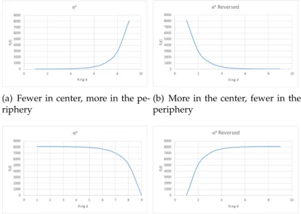
5.3.4 Exponential distribution

Finally, following the strategy of testing with different quantities of relay nodes in different parts of the network, this time we used a more aggressive distribution. In this case we have chosen to use the exponential distribution eX since it follows a very fast increase, which makes it perfect to test our hypothesis.

Figure 5.7.a shows the normal behavior of the exponential function. Fig. 5.7.b shows the same values of theeX function but in the opposite direction. Fig. 5.7.c, corresponds to the behavior when the function is negative,−eX, but applying a small modification we change the values to positive con-serving the form where we have a high number of relay nodes in the inner rings, while in the external we find very few. And finally Fig. 5.7.d, shows the behavior of the exponential function when it is negative but in reverse.

(a) Fewer in center, more in the pe-riphery

(c) More in the center, fewer in the periphery

(d) Fewer in center, more in the pe-riphery

FIGURE5.7: Exponential deployment strategy

(a) Exponential Deployment (b) Exponential Distribution

FIGURE5.8: Example of a exponential deployment follow-ing the strategy, more nodes in the center fewer nodes in the

(53)

5.3. Deployment distributions 37 5.3.5 Formulas

First, we define our base function, in this case we have chosen the value of the rings as our input parameter.

f(d) =    d=d, ifLinearDistribution, d=d2, ifQuadraticDistribution, d=ed, ifExponentialDistribution, (5.6)

Since the purpose of relay nodes is to direct the traffic and not to gener-ate any type of data, to have this type of nodes in the last ring is useless, so we distribute the quantity corresponding to the last ringf(D)among the remaining rings in equal proportion.

dist= f(D)

D−1 (5.7)

Then, we add the valuedistto our base function.

baseF unction(d) =f(d) +dist (5.8)

sumF unction= D−1

X

d=1

baseF unction(d) (5.9)

Where thebaseF unctiondepends on whether it is liner, quadratic or ex-ponential.

Now we have the linear, quadratic or exponential value,baseF unction(d) for each ring except for the last ring that does not contain relay nodes, so we setbaseF unction(D) = 0, and calculate the percentage of relay nodes that will be allocated following a distribution,5.6.

Distribution(d) = baseF unction(d)

sumF unction (5.10)

Finally we calculate the number of relay nodes that will be added to each ring.

Rd=Distritution(d)∗N r (5.11)

Having the information of how many nodes of relay class will be added per ringRd, we calculate the new percentage of nodes of normal class and relay class per ring.

relayP erRingd= Rd nodesd (5.12) normalP erRingd= Nd nodesd (5.13) wherenodesdis the total number of nodes of both classes in the rindd.

The deployment of extra relay nodes around the sink in order to solve the energy imbalanced problem in Wireless Sensor Networks

UNIVERSIDAD

POLITÉCNICA DE

C

ATALUÑA

M

T

The deployment of extra relay nodes

around the sink in order to solve the

energy imbalanced problem in

Wireless Sensor Networks

Declaration of Authorship

Abstract

Acknowledgements

Contents

List of Figures

List of Tables

To my parents, Juan and Socorro, my sisters Annel,

Anahi and Dianey who are always in my thoughts. . .

Chapter 1

Introduction

1.1

Wireless sensor networks

1.2

Motivation

1.3

Goals

Chapter 2

State of the art

2.1

The energy hole problem

2.2

The node distribution strategies

2.3

The energy efficient design

2.4

Mac Protocols

Chapter 3

Models and equations

3.1

Network model

3.2

Traffic model

3.3

Radio model

3.4

MAC protocol Model

3.5

System energy model

3.6

Delay model

3.7

The bottleneck constraint

Chapter 4

Dutycycle MAC protocols

-Energy conservation

4.1

X-Mac Protocol Analysis

4.2

X-Mac Protocol Optimization

Chapter 5

Adding extra relay nodes

5.1

Why Add extra relay nodes?

5.2

New traffic model

5.3

Deployment distributions