Visualizing Structured Data About Music
the k-pie network layout algorithm and applications to music data
Kurt Jacobson
Centre for Digital Music Queen Mary University of LondonMile End, London, UK E1 4NS
[email protected]
Mark Sandler
Centre for Digital Music Queen Mary University of LondonMile End, London, UK E1 4NS
[email protected]
ABSTRACT
In an effort to move towards intuitive visual interfaces for faceted browsing of structured data about music, we develop a visualization technique calledk-pie. Derived from a net-work visualization technique know ask-cores decomposition, k-pie layout accounts for the semantic labels or ‘colors’ asso-ciated with each vertex. Vertices of a graph are arranged in a 2 dimensional circle where ‘slices’ in the circle correspond to a specific vertex label and the most connected vertices are found in the center of the visualization. We describe the k-pie algorithm and demonstrate how it can be useful in the context of Semantic Web technologies.
Keywords
k-pie layout, k-cores decomposition, complex networks, Se-mantic Web, music, visualization
1.
INTRODUCTION
Just as music is an important part of every culture, music is an important part of on-line culture. With the ubiquity of digital music on-line, we see an opportunity to realize the promise of Semantic Web technologies and bring exciting and innovative music experiences to the end user. Significant headway has already been made in developing ontologies for the music domain [1], re-describing on-line music-related data in a structured way [2], and automatically inter-linking music collections to the Semantic Web [3]. These efforts are helping to create a Web of structured data about music - a Global Music Graph - that can be leveraged for mu-sic discovery, intelligent mumu-sic recommendation, metadata augmentation, digital rights management, and many other applications. We are now interested in making this power-ful infrastructure palatable and accessible to the expert and non-expert users alike.
In this work we develop an algorithm for visualizing large amounts of structured data. We call this algorithmk-pie. The algorithm is essentially an extension of the graph layout algorithm know ask-cores decomposition developed in [4]. Howeverk-pie differs in that it accounts for vertex labels or ‘color’. Vertices of a graph are arranged in a 2 dimensional circle where ‘slices’ in the circle correspond to a specific ver-tex label and the most connected vertices are found in the center of the visualization.
WebSci2009 Athens, Greece
By applying concepts from complex networks research to se-mantic graphsk-pie creates meaningful visualizations of the relationships between hundreds of thousands of individuals. By assigning an object property or a set of object properties as edges and a set of object classes or individuals as labels, k-pie visualizations can be created by parsing results from the SPARQL query language [5].
The rest of the paper is organized as follows. In Section 2 we briefly review some related work. In Section 3 we describe thek-pie algorithm and show how it can be used in the con-text of structured data. In Section 4 we show some of the applications of thek-pie method including the visualization of Myspace music artists and visualization of influence be-tween classical composers. Finally in Section 5 we provide a discussion and ideas for future work.
2.
BACKGROUND
As mentioned above, the k-pie algorithm is a rather intu-itive extension of the network visualization algorithmk-core decomposition developed by Alvarez-Hamelin et. al in [4]. The k-core decomposition algorithm begins with a k-core analysis on a given graph structure and places vertices in a 2 dimensional space using a pair of polar coordinates - a radius related to the shellness of a given vertex and an angle related to the cluster of that vertex after k-cores analysis. We will review these concepts again in Section 3.1.
We are most interested in visualizing data about music artists. We describe this data using Music Ontology terms and other supporting Web onotolgies following the work of Raimond [1]. We are interested in utilizing thek-pie visualization al-gorithm as a tool for interacting with structured data on the Semantic Web [6]. There exists a growing number of tools for visualizing and browsing structured data [7].
3.
ALGORITHM
To describe the k-pie algorithm first we will provide some definitions and concepts associated with thek-core decom-position algorithm.
3.1
Definitions
Let us consider a graphG= (V, E) where|V|=nvertices and |E|=e edges. As described in [8], ak-core is defined as follows:
Definition 1. A subgraph H = (C, E|C) induced by the set C ⊆ V is a k-core or a core of order k iff ∀v ∈ C :
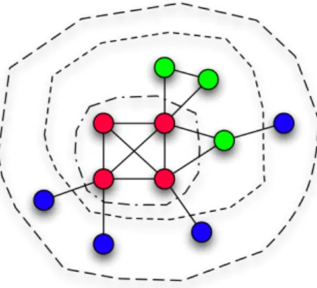
Figure 1: The k-core decomposition for a small graph. Each closed line contains the set of vertices belonging to a given k-core, and the color of the vertices distinguish differentk-shells.
degreeH(v)≤k, andHis the maximum subgraph with this property.
Definition 2. A vertexihas ashellness cif it belongs to thec-core but not to the (c+1)-core. We denote the shellness of vertexibyci.
Definition 3. AshellCcis composed of all vertices whose shellness is c. The maximum value c such thatCc is not empty is denotedcmax. Thek-core is then the union of all
Ccwithc≥k.
It is important to note the distinction between ak-core and ak-shell - ak-shell implies a certain range of vertex degrees while ak-core only implies a lower limit to vertex degree. We are more interested ink-shells for our visualization al-gorithm.
In thek-core analysis all vertices of a connected graph belong to the 1-core. In Figure 3.1 this is indicated by the largest line encircling the entire graph. Then, all vertices of degree d <2 are recursively cut out. In Figure 3.1 these are the blue vertices and they constitute the 1-shell. All other vertices maintain a degree ofd≥2 after pruning the blue vertices, and are not eliminated in this step. The remaining vertices form the 2-core, enclosed by another dotted line. In the next step vertices with degreed <3 are pruned revealing the 3-core. Note thatcmax= 3 in the graph in Figure 3.1 as after pruning no vertex has a degree d >3. Also note that the coloring of the vertices in the Figure indicate their shellness. In addition to the above definitions, let us also consider that each vertexihas a label associated with itli and L is the set of all labels found in the graphGandsis the number of distinct labels found inL.
3.2
Layout equations
Thek-pie visualization algorithm positions vertices in 2 di-mensional space. The position of each vertex depends on its
shellness and its semantic label. Each vertexiis positioned using a pair of polar coordinates (ρi, αi). The radiusρi de-pends on the shellness of iand that of its neighbors while the angle αi depends on the label associated with i. In the resulting visualization, k-shells are presented as layers of concentric circles with the innermost circle correspond-ing to the vertices with the highest shellness. Then vertices sharing the same label are positioned within in a certain an-gular range. This creates pie-like ‘slices’ of vertices sharing the same label across thek-shell layers. Hence the name of the algorithmk-pie.
The calculation ofρi is as follows:
ρi= (1−)(cmax−ci) + |Vcj ≥ci(i)| X j∈Vcj≥ci(i) (cmax−ci) (1) whereVcj ≥ciis the set of neighbors ofihaving shellnesscj
greater or equal toci. The parameteris a tuning parameter to control the possibility of rings overlapping.
Then, the angleαiis calculated as follows:
αi= 2π X 1≤m<li |Lm| n +N „ |Lli| 2n , 2π|Lli| n « (2) whereLis an ordered list of the labels in the graph and|Lm| is the number of vertices with the label m,N is a normal distribution of mean |Lli|
2n and width 2π|Lli|
n . AssumingL is an ordered list of labels, referring tom < li allows us to allocate the appropriate portion of the angular space to a given label.
3.3
Color and size of vertices and edges
The size of each vertex in the visualization corresponds to the logarithm of its degree. Generally, the larger (higher degree) vertices be nearest the center of the visualization although it is possible for a higher degree vertex to exist in one of the more outer shells.
The coloring of the vertices is related to the label associated with each vertex. Each distinct label found in Lis given a unique color.
The drawing of edges can be considered optional. In fact drawing all the edges in a larger graph will result in an unintelligible tangle. With no edges drawn at all, the result-ing visualization is still useful. A homogeneously randomly sampled fraction of edges can be drawn. This approach does not add to computational cost significantly and is used in [4]. A more computationally expensive approach is to only draw edges with a higherbetweenness centrality- those edges which are found more often in the shortest paths between a pair of vertices [9].
3.4
Complexity
Thek-pie algorithm has a complexity that is nearly identical to that ofk-core decomposition. If we assume no re-ordering ofLwe can index our list of labels for the angular calculation inO(s∗n) wheresis the number of labels. Generallyswill be small compared tonthe number of vertices. Thek-core
decomposition takes time O(n+e) - O(n) to build a list of vertex’s degeree andO(e) to perform the pruning in the recursive decomposition step whereeis the number of edges. So our total time complexity fork-pie isO(s∗n+n+e) or simplyO(n+e) if the number of distinct labelssis small.
4.
APPLICATION
Thek-pie algorithm could be applied to most any graph-like data that includes vertex labels of some kind. Here we will discuss the application that motivated our development of k-pie - visualization of the Myspace artist network.
First discussed in [2] the Myspace artist network consists of a subset of the Myspace social network that includes only users who specify that they are ‘artists’. A network is con-structed from the directed ‘top friend’ relationship between pairs of artists. This relation is chosen over the general undirected ’friend’ relation because it is assumed to be more meaningful and salient in terms of musical similarity. That is to say, a ‘top friend’ relationship is more likely to imply some musical relationship between two artists - collabora-tion, co-membership, or stylistic influence.
The data set from [2] was republished as structured data in RDF and a live wrapper service1 was created to dereference Myspace-related URIs on demand.
We want to create ak-pie visualization where the vertices are Myspace music artists, the vertices’ labels are the musical genre labels specified by the artists on Myspace, and the edges are top friend relationships to other artists. We can fetch this data using the SPARQL query language and the endpoint containing out data set2. The query is as follows
PREFIX myspo:<http://purl.org/ontology/myspace#> SELECT ?from ?to ?fromLabel ?toLabel
FROM <http://dbtune.org/myspace-fj-2008> WHERE{
{?from myspo:topFriend ?to . } OPTIONAL{
?from myspo:genreLabel ?fromLabel . ?to myspo:genreLabel ?toLabel} }
After execution the “from” and “to” fields will specify our directed edge list for constructing our graph. The “fromLa-bel” and “toLa“fromLa-bel” will contain the labelslifor each vertexi. We specify these triple patterns as “OPTIONAL” to include vertices that have no genre label specified.
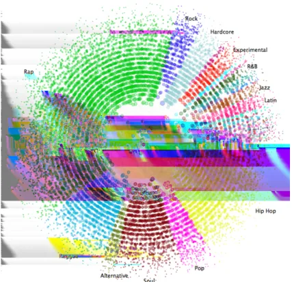
We can see the results of this query and visualization in Fig-ure 2. Each vertex represents a music artist and the color of each vertex indicates the primary genre label associated with that artist. This data set contains n = 15,019 ver-tices (music artists) ande= 114,606 edges (top friend rela-tions) ands= 106 labels (genre). Notice that a few highly 1available athttp://dbtune.org/myspace
2
available athttp://dbtune.org/sparql
connected music artists gravitate towards the center belong-ing to the highestk-shells aroundcmax= 29. However the shells immediately lower thancmax are mostly empty. This behavior is indicative of scale-free networks where the cumulative degree distribution follows a power law decay -Pc(d) ∼d−(α−1) [10]. Also note that the highly connected vertices in the centerk-shells constitute a “rich club” where the music artists with the highest degree values are also con-nected to each other [11]. We can also get a sense for what musical genres dominate this sample of the Myspace artist network. We can see that “Hip Hop” (yellow) and “Rap” (bright green) account for nearly half of all the genre labels in the data set. We also see that the rich club in the center of the visualization includes vertices with genre labels “Hip Hop”, “Rap”, “Soul”, “Reggae”, and “Hardcore” - a somewhat surprising addition to the list. Note that the genre label ap-pears as text only for those genre labels that are associated with more than 1% of the vertices in the network. The data set actually includes 106 unique genre labels and therefore the visualization contains 106 distinct colors. However, it can be exceedingly difficult for the viewer to accurately dis-tinguish between so many colors therefore text labels are used in favor of a color legend. The vertices are drawn to be translucent so the viewer can get a better sense vertex concentration where vertices fall on top of one another. In this visualization only 0.2% of the network edges are chosen uniformly at random and included in the visualization. The remainder of the edges are ignored.
Thek-pie algorithm has also been applied to a data set of classical composers and the network of influence between composers.3 This data set is essentially a re-publication of the data about classical composer influence compiled by Charles H. Smith in the 1990’s for the Classical Music Navi-gator (CMN) website [12]. Following the Linked Data guide-lines for publishing structured data on the Web [13], this data set contains links to the DBpedia data set.4 We can follow these links to obtain additional data about the com-posers. Of the 444 composers in the CMN data set, we have obtained links to DBpedia for 245. Thek-pie algorithm can be used to visualize the data using, for example, “rdf:type” or “dbpedia:birthPlace”, as the vertex label parameter. A small proof-of-concept software package has been developed to visualize this small data set.5
5.
DISCUSSION AND FUTURE WORK
The k-pie layout algorithm allows for the creation of use-ful and intuitive visualizations of large collections of labeled network data. This algorithm can be useful in the context of the Semantic Web and combined with technologies like SPARQL to create visualizations of moderately large sets of structured data. A quick inspection of the visualization gives the viewer a sense of the make up of the network in terms of labels and a sense of what labels are associated with the most connected vertices.
However there are some difficulties with thek-pie algorithm in its current state. Perhaps most notably, there is no clear method for ordering the list of vertices’ labelsLfound in the 3
available at: http://dbtune.org/cmn 4http://dbpedia.org
5
Figure 2: k-pie layout visualization of a sample of the Myspace artist network where the slices and vertex colors correspond to genre labels. Note that genre label text is only printed for genre labels that constitute
>1% of vertex labels.
target graph. In the current implementation, L is naively ordered as the labels appear when constructing the graph - the label that is found first appears as the first label in L. The ordering ofLdictates the ordering of the ‘slices’ in the visualization. It would be preferable if this ordering had some meaning or justification. One option would be to build an adjacency matrix for the labels inL and approach this as a circular layout problem and use a method like spectral re-ordering [14] to organize the labels. This would have the effect of placing the most connected labels in the original graph closer together in the re-ordered list.
Another short coming of thek-pie algorithm is that it allows for each vertex to be associated with only one label. This is often at odds with the complexity of real world entities and their descriptions on the Semantic Web, which by design, allows for an entity to be associated with many labels. Even in our Myspace music artist genre application, we naively se-lect only the first genre label associated with a given artist assuming it is the most important. According to the inter-face design of Myspace, an artist may have between 0 and 3 genre labels. We simply ignore the additional labels in the visualization. To the best knowledge of the authors, there is no clear way to address multiple labels in the context of thek-pie layout algorithm.
As can be seen in 2 nodes tend to bunch together in large graphs. Although the viewer can clearly see what portion of the vertices are associated with different labels and which vertices are the most connected in the graph, much of the
detail is lost. For this reason we purposek-pie is most appro-priate for generating global over views of medium to large data sets and would be most effective as one aspect of a multi-view interactive data exploration experience.
Because the complexity ofk-pie is relatively low, it could be incorporated into a faceted browsing interface where thek -pie layout is re-caclulated as the browsing context changes. In future development we hope to use k-pie visualizations in a read-write tool for RDF data following the principles outlined in [15].
Currentlyk-pie requires the construction of ad hoc SPARQL queries to visualize data sets published on the Semantic Web. The original aim was to develop a more general frame-work for visualizing structured data and Linked Data [13]. Unfortunately the current work falls short of this aim and fo-cuses instead on a basic network visualization algorithm and its application to a specific Semantic Web data set. Creat-ing a more general framework for visualizCreat-ing and interactCreat-ing with Linked Data and structured data on the Semantic Web is a primary goal of future work.
6.
WEB RESOURCES
The following Web resources supplement the material pre-sented in this work:
• An open-source Java implementation ofk-pie available by svn checkout athttp://grasstunes.net/subclipse/ KPieLayout
• Fields-Jacobson Myspace data available via SPARQL athttp://dbtune.org/sparql
• Myspace RDF wrapper service available at http://dbtune.org/myspace
• Classical Music Navigator data set available at http://dbtune.org/cmn
• Classical Music Universe data browser available at http://omras2.org/ClassicalMusicUniverse
7.
ACKNOWLEDGEMENTS
The authors would like to acknowledge Ben Fields at Gold-smiths University of London for his assistance in collecting the original Myspace data set. This work is supported as a part of the OMRAS2 project, EPSRC grants EP/E02274X/1 and EP/E017614/1.
8.
REFERENCES
[1] Y. Raimond, “A distributed music information system,” Ph.D. dissertation, Queen Mary University of London, 2009.
[2] K. Jacobson and M. Sandler, “Musically meaningful or just noise, an analysis of on-line artist networks,” in
Proc. of CMMR, 2008, pp. 306–314.
[3] Y. Raimond, C. Sutton, and M. Sandler, “Automatic interlinking of music datasets on the semantic web,” 2008.
[4] J. I. Alvarez-Hamelin, L. Dall’Asta, A. Barrat, and A. Vespignani, “k-core decomposition: a tool for the visualization of large scale networks,”CANADA, p. 41, 2006. [Online]. Available:
http://www.citebase.org/abstract?id=oai:arXiv.org: cs/0504107
[5] “SPARQL query language for RDF, W3C recommendation,” 2008. [Online]. Available: http://www.w3.org/TR/rdf-sparql-query/ [6] T. Burners-Lee, J. Hendler, and O. Lassila, “The
semantic web,”Scientific American, vol. 284, no. 5, May 2001. [Online]. Available:
http://www-sop.inria.fr/acacia/cours/essi2006/ Scientific%20American %20Feature%20Article %20The%20Semantic%20Web %20May%202001.pdf [7] S. Kushro and A. Tjoa, “Fulfilling the needs of a
metadata creator and analyst- an investigation of rdf browsing and visualization tools,”Canadian Semantic Web, pp. 81–101, 2006. [Online]. Available:
http://dx.doi.org/10.1007/978-0-387-34347-1 6 [8] V. Batagelj and M. Zaversnik, “Generalized cores,”
2002. [Online]. Available:
http://www.citebase.org/abstract?id=oai:arXiv.org: cs/0202039
[9] L. C. Freeman, “A set of measures of centrality based on betweenness,”Sociometry, vol. 40, no. 1, pp. 35–41, 1977.
[10] M. E. J. Newman, “The structure and function of complex networks,”SIAM Review, vol. 45, p. 167, 2003. [Online]. Available:
http://www.citebase.org/abstract?id=oai:arXiv.org: cond-mat/0303516
[11] L. F. Costa, F. A. Rodrigues, G. Travieso, and P. R. V. Boas, “Characterization of complex networks:
A survey of measurements,”Advances In Physics, vol. 56, p. 167, 2007. [Online]. Available:
doi:10.1080/00018730601170527
[12] The classical music navigator. [Online]. Available: http://www.wku.edu/˜smithch/music/
[13] C. Bizer, R. Cyganiak, and T. Heath. How to publish linked data on the web. [Online]. Available:
http://linkeddata.org/docs/how-to-publish [14] D. J. Higham, G. Kalna, and M. Kibble, “Spectral
clustering and its use in bioinformatics,”J. Comput. Appl. Math., vol. 204, no. 1, pp. 25–37, 2007. [Online]. Available:
http://portal.acm.org/citation.cfm?id=1238339 [15] T. Berners-Lee, J. Hollenbach, K. Lu, J. Presbrey,
E. P. d’ommeaux, and m.c. schraefel, “Tabulator redux: Writing into the semantic web,” 2007. [Online]. Available: http://eprints.ecs.soton.ac.uk/14773/