Road Project Investment Evaluation Using Net Present Value (NPV) at
Risk Method
Swapan Kumar Bagui
1)and
Ambarish Ghosh
2)1) Corresponding Author, Bengal Engineering and Science University, Shibpur, Howrah - 711 103, India. E-Mail: [email protected] & [email protected]
2)
Professor, Bengal Engineering and Science University, Shibpur, Howrah - 711 103, India. E-Mail: [email protected]
ABSTRACT
Strategic capital investment decisions are crucial and require careful analysis and consideration. This is due to the characteristics of infrastructure projects that are vulnerable to risks and uncertainties. Net Present Value (NPV)-at-Risk model developed by Ye and Tiong (2000) is a tool for investment evaluation under uncertainties. This paper presents an extension of the model to determine NPV at risk proposed by Ye and Tiong (2000). NPV at risk has been determined using three discount methods, cash flow after payment of tax, interest and principal debt, and the results were compared to choose the best one. NPV at risk was also determined using normal distribution and Monte Carlo simulation method with varying debt equity ratio. The evaluation of the road project shows that the NPV-at-risk method can provide a better decision for risk evaluation and investment in privately financed road projects. This paper presents NPV at risk and return at this NPV with a real case study.
KEYWORDS: Capital investment, Vulnerability to risk and uncertainties, NPV at risk, Road projects.
INTRODUCTION
Strategic capital investment decisions are crucial to a business firm. The decision to become involved in privately financed infrastructure projects such as a Build Operate Transfer (BOT) toll road requires careful consideration and thorough analysis. Traditionally, investment decisions on infrastructure projects are made by the investing government based on the benefit-cost analysis and economic viability of the projects. The primary objective of the private sector is to maximize profit, and its decisions are mainly based on the financial viability of projects.
The most common methods for the assessment of financial viability are: the payback period, average
accounting rate of return, Net Present Value (NPV) and Internal Rate of Return (IRR) methods. Decisions derived from these methods are based on the forecasts of base-case cash flows. However, BOT infrastructure projects are characterized by high capital outlays, long lead times and long operating periods. These characteristics make the forecasts of cash flows more difficult and expose the private sector to high levels of financial, political and market risks. This requires the decision to incorporate risk analysis into project appraisal methods. Financing is a key element of BOT projects; investment decisions also should take financing methods into account. A more vigorous investment decision method that incorporates both risk and financing methods is needed. This paper develops an improvement of the project evaluation method Accepted for Publication on 14/2/2012.
NPV-at-risk developed by Ye and Tiong (2000) and attempts to show that this method can potentially overcome these problems in investment decision making.
METHODS OF CAPITAL INVESTMENT
DECISION MAKING
The project evaluation methods may systematically be classified into three categories: methods based on return, methods based on risk and methods based on both return and risk. The methods based on return include the payback period, the average accounting rate of return (also called the return on capital employed), NPV and IRR. The payback period and the average accounting rate of return methods ignore the time value of money, whereas NPV and IRR methods incorporate the time value of money into decision making using discounted cash flow techniques. But all of them are based on the assumption that the cash flows of the project are certain, whereas the project’s actual cash flows could substantially differ from the forecast cash flows. The uncertainties bring risk into capital investment evaluation decisions. This directs attention to the development of risk-rating systems. Investors must determine their own required returns. The inadequacies of a decision criterion based solely on return or risk show that methods incorporating risk into the measurement of return should be developed. The most common methods are the risk-adjusted discount rate methods such as Capital Asset Pricing Model (CAPM), Arbitrage Pricing Theory (APT) and the Weighted Average Cost of Capital (WACC).They focus on the determination of discount rates under uncertainties. The philosophy of these methods is that the risk adjusted discount rate should consist of risk free rate and risk premium. A major problem with the methods is that there is no indication of confidence level on the determined discount rate. An alternative approach is probabilistic. NPV-at-risk is a method that attempts to show that this method can potentially overcome these problems in investment decision making.
LITERATURE REVIEW
NPV at Risk
One of the six definitions of risk listed by Vlek and Stallen (1981) is that risk is the semi-variance of the distribution of all consequences, taken over negative consequences only, and with respect to some adopted reference value. The semi-variance alone as the measure of risk is not sufficient to make a decision, but it can be combined with the expected NPV to form a new decision rule; a project is acceptable if the mean NPV minus the standard deviation is greater than zero. However, this decision rule fails to provide decision-makers with a confidence level; Instead of calculating the mean NPV and standard deviation, the NPVa at a given confidence level is computed so that the decision rule is that the project is acceptable with the given confidence level if the NPVa is greater than zero. Based on this consideration, NPV-at-risk is defined as a particular NPV that is generated from a project at some specific confidence level; that is, the minimum expected NPV with the given confidence level. According to the definition of NPV-at-risk, the following decision rules can be derived: the project is acceptable with a confidence level of 1 - α if NPV-at-risk at the given confidence level is greater than zero; otherwise, it is unacceptable. The NPV-at-risk method aims to calculate the value that the project’s NPVs will be greater than, with the probability corresponding to the given confidence level. It involves the determination of discount rate and the generation of cumulative distribution of possible NPVs. To calculate NPV, the key task is to determine an appropriate discount rate.
CAPM model and APT were developed for financial markets, their application to stand-alone projects suffers from the difficulty in determining appropriate beta. Moreover, the discount rate determined by these methods may overemphasize (double count) the impact of risk exposure because the NPV-at-risk method will also take the risk into account. Unlike CAPM and APT, WACC is the cost of various financial sources weighted by their corresponding proportions in the overall pool of
financing. The cost of a financial source is the return expected by investors. According to Tiong (1995), the equity of a BOT project is usually about 20-30% of the total investment, and the remainder is debt finance. The equity required return is assumed to be the hurdle rate of sponsors, whereas the debt required return is assumed to be the average market interest rate. Determined in this way, WACC does not sufficiently reflect the required risk premium. Moreover, according to Farid et al. (1989), WACC is the only practicable option at the present time. But this does not mean that WACC alone is good at handling risk. Therefore, the use of WACC for determining the discount rate in the NPV-at-risk method is practicable without overestimating risk. In addition, WACC enables the NPV-at-risk method to take financing methods into account. According to the requirements of decision rules, there are two approaches to investment decision making, the calculation of NPV at a given confidence level and the calculation of a confidence level at the point of zero NPV. When the project’s NPVs are normally distributed, the NPV-at-risk can be obtained through the mean variance method. Alternatively, assuming that the cumulative distribution function of return is F(NPV), NPV-at-risk at a given confidence a and the confidence level at the point of zero NPV can be obtained using percentile analysis on the cumulative distribution. If the distribution functions of return, f(NPV) or F(NPV), are unknown, Monte Carlo simulation can be used to generate the distribution of possible NPVs. Ye and Tiong (2000) developed NPV at Risk Model. They used WACC method for calculating discount rate and cash flow taken before tax.
Discount Rate
Choosing the appropriate discount rate for present value analysis of a project under simulated environments remains the subject of international debates. There is no substantial consensus whether the risk-free rate or the opportunity cost of capital, which can also be the opportunity cost of debt or the cost of equity if dealing with source of financing, should be
chosen. Malini (1999), for instance, implicitly suggested the use of the opportunity cost of equity, which includes a risk premium and the borrowing rate of long-term debt. In developing the NPV at risk method, Ye and Tiong (2000) used the weighted average cost of capital (WACC). They stated that the capital asset pricing model (CAPM) and arbitrage pricing theory (APT) suffer from the difficulty in determining appropriate beta. Determining WACC is not less difficult because a financial manager needs to estimate the cost of debt and the cost of equity, the principal components of WACC, which are sometimes derived from CAPM. Additionally, the use of WACC is based on the assumption that the firm can maintain a constant leverage ratio, thus requiring rebalancing capital structure over the project’s life. This requirement is difficult to meet in project finance where it typically means very high debt ratio from the beginning, with most or all of a project’s early cash flows committed to debt service, meaning that equity investors have to wait (Brealey and Myers, 2000). Savvides (1994) and Hacura et al. (2001) believe that the appropriate discount rate for calculating the present value of a project in the stochastic appraisal is that used in the deterministic appraisal. On the contrary, Brealey and Myers (2000) argue that the risk-free rate instead of the opportunity cost of capital should be used in order to avoid prejudging risk because if the opportunity cost of capital is known, simulation is not necessary except for helping forecast cash flows. In another context, Handa (1995) and Byrne (1996) applied the risk-free rate for project valuation under uncertainty using variance analysis where risk is let to reside in cash flows, which are then discounted at the risk-free rate. In this case, the project’s NPV itself is considered a random variable. This is a very different approach from that of single value estimates (deterministic) to risk analysis in which the discount rate needs to be adjusted as risk changes. In the present work, the risk-free rate is used to discount uncertain cash flows of involved parties so that analysis can be made on a similar basis.
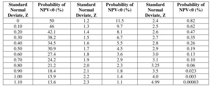
Table 1. Standard Normal Deviate Value Corresponding to Percentage of NPV <0 Standard Normal Deviate, Z Probability of NPV<0 (%) Standard Normal Deviate, Z Probability of NPV<0 (%) Standard Normal Deviate, Z Probability of NPV<0 (%) 0 50 1.2 11.5 2.4 0.82 0.10 46 1.3 9.7 2.5 0.62 0.20 42.1 1.4 8.1 2.6 0.47 0.30 38.2 1.5 6.7 2.7 0.35 0.40 34.5 1.6 5.5 2.8 0.26 0.50 30.9 1.7 4.5 2.9 0.19 0.60 27.4 1.8 3.6 3.0 0.13 0.70 24.2 1.9 2.9 3.1 0.10 0.80 21.2 2.0 2.3 3.25 0.06 0.90 18.4 2.1 1.8 3.5 0.023 1.00 15.9 2.2 1.4 4.0 0.003 1.10 13.6 2.3 1.1 4.99 0.00003
LEAD FROM PAST STUDY
NPV at risk can be also determined using other methods of discount rate, and cash flow after tax payment should be considered for the determination of NPV at risk. In a road project after construction, major risk is revenue /tollable traffic. Traffic may be reduced after construction. Return on NPV at risk may be determined varying traffic at NPV risk by trial and error method.
OBJECTIVE AND SCOPE
Based on previous works and past studies, it is felt that NPV at risk and internal rate of return at risk (various confidence levels) can be determined with a real case study considering cash flow after tax and discount rate proposed by Chen (1998), Shen and Li (2002) and WACC methods:
Discount rate proposed by Chen (1998) :
1 Equity(% ) ROE Debt(% ) Debt of Interest Rate Discount Alternatively, it can be written as:
E D E r E D D r Rate Discount d e (2) where, rd=Cost of Debt; re=Cost of Equity; D=Debt; E=Equity.
Shen and Li (2002) proposed another formula to calculate discount rate as mentioned below:
1 I 1 I 1 Rate Discount nf (3) where, I = Interest rate; Inf = Inflation Rate.
This method provides better NPV and investment makes good profits from the project.
Discount rate by WACC method can be determined as:
E D E r E D D tax)r (1 Rate Discount d e (4) where,
Tax =Corporate Tax Rate.
PROPOSED METHODOLOGY
The proposed methodology to determine NPV at risk is described below.
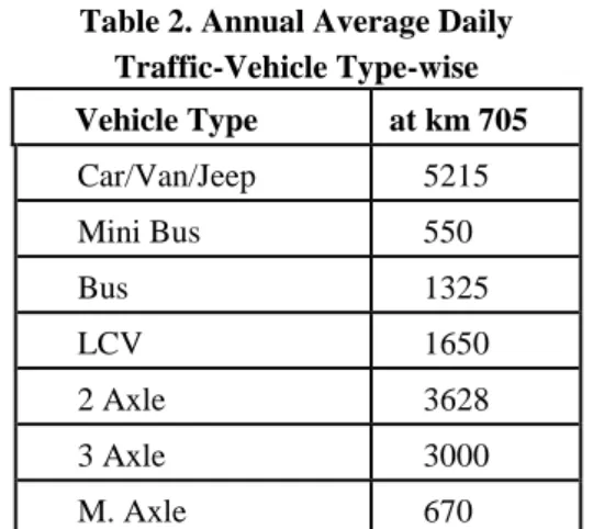
Table 2. Annual Average Daily Traffic-Vehicle Type-wise Vehicle Type at km 705 Car/Van/Jeep 5215 Mini Bus 550 Bus 1325 LCV 1650 2 Axle 3628 3 Axle 3000 M. Axle 670
Cash flow of equity is considered after interest and tax payment. Discount rate is calculated using Equations 1,2,3 and 4. Interest rate of debt and return on equity is considered risk-free value to avoid double counting risk (Chandra, 2005).
The following steps are considered to determine NPV at risk.
Case a: Assuming NPV is normally distributed function:
1.
Determine total NPV, NPVt and average NPV,NPVa during concession period.2.
Determine standard deviation of NPV,σ during concession period.3.
Determine Z using the following formula:σ NPVt) (0
Z
4.
Reliability of data can be obtained from Table 1.5.
NPV at risk can be determined as: NPV at risk=NPVa-Z(σ)6.
Calculate FIIR at risk, reducing traffic level of base case by trial and error method at NPV risk. Case b: Assuming NPV is cumulative distributedfunction:
7.
Alternatively, prepare cumulative distribution graph of NPV to determine NPV at risk.Case c: Assuming NPV distribution using Monte Carlo Method.
CASE STUSY
Project road corridor is a section of 79A, NH-79 and NH-76 starting from Kishangarh (km 364.00 of NH-8). It meets with NH-79 at km 14.10 after traversing 36.0 km up-to Chittorgarh (km 183.00) and (km 220.00 of NH-76) via Chittorgarh and meets Udaipur Bypass at km 117.8. The length of the Udaipur By-pass is 11.1 km which is under construction. The road passes through the important towns of Nasirabad (km 14.00 of NH-79), Bhilwara (km 120.23 of NH-79), and Chittorgarh (km 183.00 of 79) in the Rajasthan State. The existing road is a 2-land divided carriageway. The length of the by-pass is 29.6 km. With this, the overall length of the project road including by-pass length in Chittorgarh is 315 km. The manual seven days traffic volume counts were carried out (November 1999) at km 205.
The Annual Average Daily Traffic (AADT) values are used for future projections for a 30 year analysis period. Growth rate factors are taken as 5 % as recommended by Model Concession Agreement, NHAI, 2000. Tollable traffic count for Section Chittorgarh Bypass (km 213.6 to km 174.0) is shown in Table 2.
Toll Rate
The toll rate is selected using guidelines prepared by the Government of India. The inflation rate has been determined based on: Reserve Bank of India Bulletin, 2000.Whole price index for all commodities is found to be 8.3%. Using this value, the future toll rate has been projected for future year, and the toll rate for the opening year, 2004, is mentioned in Table 3. Toll rate increasing factor for the year 2004 is 1.0837=1.74.
Project Cost
The project cost has been worked out and found to be Rs 40 million.
Financial Analysis
following major maintenance and operation costs into account:
Annual Routine Maintenance (repair of pot hole, clearing C D structure… etc.) Cost (Rs 0.2 million per km).
Periodic Maintenance (Overlay every 5th year) Cost (Rs 2.8 million per km).
Toll Operation (Toll administrative cost) Cost (Rs 6 million for toll plaza per year).
Table 3. Toll Rate Per /km Vehicle-wise
Year Car Full Bus Multi Axle LCV 2A,3A Truck Toll Rate Rs (1997) 0.40 1.40 3.00 0.70 1.40 Toll Rate Rs (2004)* 0.69 2.40 5.20 1.20 240
Toll Rate Rs (2008) 0.96 3.36 7.2 1.68 3.36 Note: Toll rate in 2004 is obtained by multiplying toll rate of 1997 by 1.74.
Table 4. NPV at Various Equity and Confidence Levels
Equity (%) NPV(Rs Million)
Base Case 95% Con. Level 97% Con. Level 99% Con. Level
10 1094 45.2*/50** 43/42.2 40/34
20 830 31.9/32.9 30.3/27.5 28.4/21.6
30 582 21.2/20.3 20.8/18 19.5/15
40 351 12.5/10.6 11.9/9.6 11.4/7.9
50 135 4.8/3.8 4.6/3.3 4.3/3.1
Note:* for COV =0.1,**for COV=0.2.
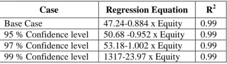
Table 5. Regression Equations and R2 Values
Case Regression Equation R2 Base Case 47.24-0.884 x Equity 0.99 95 % Confidence level 50.68 -0.952 x Equity 0.99 97 % Confidence level 53.18-1.002 x Equity 0.99 99 % Confidence level 1317-23.97 x Equity 0.99
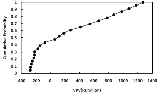
Financial analysis is carried out varying equity from 10 to 50 %. The concession period is taken 23 years (3 years construction period+20 years operation period) and the payback period is taken 10 years. Interest on debt and return on equity are assumed 15 % and 20%. NPV distribution graph has been plotted and shown in Fig.1 for an equity of 10 %.
NPV-at-risk of the project at 95% confidence level is found ( - )Rs 276.9 million and the probability is found 0.46 at the point of zero NPV. Thus, the project is not investable for a debt equity ratio of 9. Decreasing debt equity ratio to 2.5, the probability of NPV < 0
increased to 0.5. Even with a debt equity ratio reduced to 0.2, the probability of NPV < 0 increased to 1.0. Even with a debt equity ratio of 99, the probability of NPV < 0 increased to 0.5.
From the data, it is shown that the road project is a very high risk project and the probability of risk is high. Probablity of NPV at risk at 80 to 95% confidence level is not achievable. Confidence level may be reduced to 60-70%.
To overcome this problem, normal distribution and cumulative frequency distribution methods are proposed to find out the NPV at risk. Mean value of
NPV of the equity (entire concession period) is considered to calculate NPV at risk.
In order to calculate NPV at risk, average NPV is calculated and found approximately Rs 50 million for the base case. Assumed is a standard deviation of Rs 5 million or alternatively a coefficient of variation of 0.1. Normal distribution curve has been prepared and shown in Fig.2. This curve is drawn for an equity of 10 % and a COV equal to 0.1. Similar graphs are also prepared for equities of 20,30 ,40 and 50% with COV values of 0.1 and 0.2.
NPV at various confidenence levels (95%, 97% and 99 %) and base case have been calculated varying equity from 10% to 50%. Equity beyond 50% is infeasible; hence not considered. These values are reported in Table 4. Table 4 is prepared determining the discount rate using equation 1.
For an equity proportion of 50%, NPV at risk values vary from 3 to 4.75; i.e., very small values, FIRR has been found in the range of 17.52 to 17.54 % and traffic reduction factor values vary from 0.9445 to 0.9452.
Monte Carlo Simulation Method
J. Von Neumann and S. Ulam are considered as the inventors of the Monte-Carlo method. The random number plays a fundamental role in the method. Monte-Carlo is famous for its casinos and the roulette is nothing else than a random number generator. This explains the name of the method. The method includes all numerical methods which simulate processes depending on random variables. Usually, these calculations are too complex to be solved analytically.
Random value of NPV varying between minimum and maximum can be determined using the Monte-Carlo Simulation Method.
The Monte-Carlo Simulation Method is based on the generation of multiple trials to determine the expected value of random variable. The basis of the method is provided by the following relationship:
n N Pr 1
< N 3 ≈Defined Value.There is a number of commercial packages that run Monte-Carlo Simulation; however a basic spreadsheet program can be used to run a simulation. In this case, the generation of multiple trials is implemented by propagating a basic formula as many times as the number of iterations required by the model.
Let us assume an activity has two probable ranges of values (upper limit and lower limit). Random value can be generated using this method as shown below. Determination of the Number of Iterations
The Monte-Carlo method provides an estimate of the expected value of random variable and also predicts the estimation error, which is proportional to the number of iterations.
The total error is given by:
N
3
where,
σ = standard deviation of the random variable; N = Number of iterations.
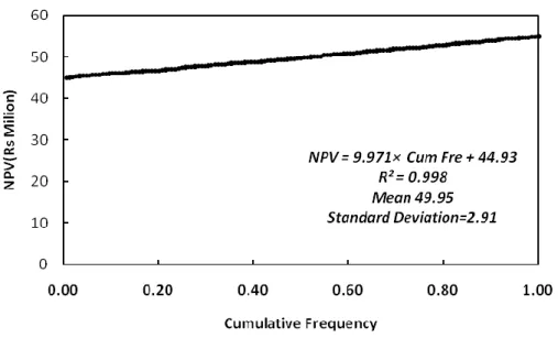
Sort random variables increasing order and frequency. Plot the cumulative diagram as shown in Fig. 3. Random variables are generated taking lower and upper limits of 45 and 55, respectively. NPV at 95% confidence level is calculated and shown below. NPV = 44.93+9.971*0.05 = 45.4.
Again, NPV=49.95-1.645*2.91=45.2.It is also found from Table 2, that NPV at 95 %confidence level=45.2.Data obtained from all these methods are comparable and close to each other. Discount rate has been calculated using equation 3. Taking an interest rate of debt of 15%, a return on equity of 20% and an inflation of 5%, discount rates of debt and equity are 9.5 and 14.3%, respectively. Some selected data are reported in Table 7. The same project is viable for an equity of 90%. Table 8 is prepared using discount rate, WACC method, as shown in equation 4.
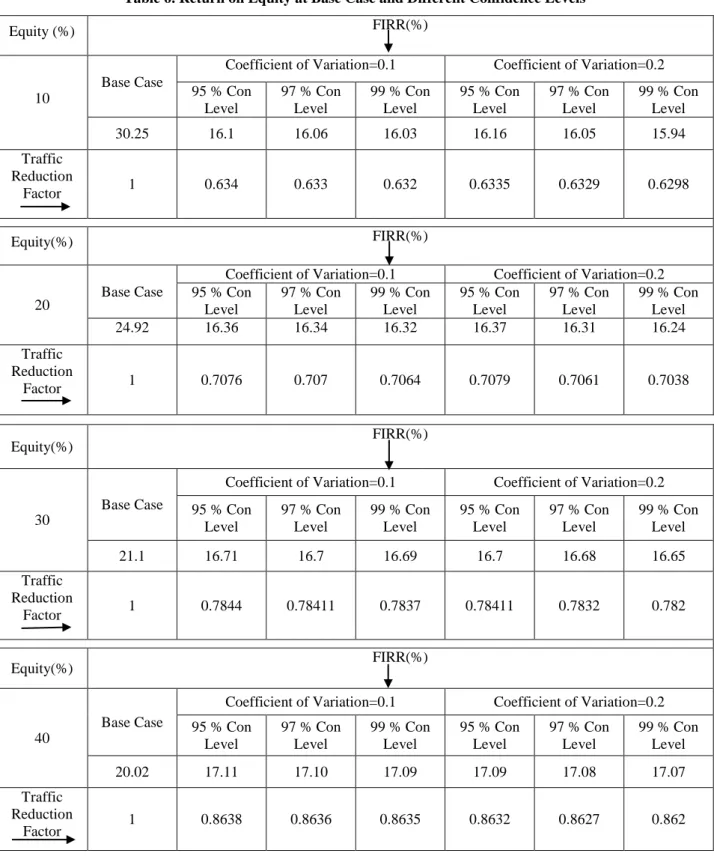
Table 6. Return on Equity at Base Case and Different Confidence Levels
Equity (%) FIRR(%)
10
Base Case
Coefficient of Variation=0.1 Coefficient of Variation=0.2 95 % Con Level 97 % Con Level 99 % Con Level 95 % Con Level 97 % Con Level 99 % Con Level 30.25 16.1 16.06 16.03 16.16 16.05 15.94 Traffic Reduction Factor 1 0.634 0.633 0.632 0.6335 0.6329 0.6298 Equity(%) FIRR(%) 20 Base Case
Coefficient of Variation=0.1 Coefficient of Variation=0.2 95 % Con Level 97 % Con Level 99 % Con Level 95 % Con Level 97 % Con Level 99 % Con Level 24.92 16.36 16.34 16.32 16.37 16.31 16.24 Traffic Reduction Factor 1 0.7076 0.707 0.7064 0.7079 0.7061 0.7038 Equity(%) FIRR(%) 30 Base Case
Coefficient of Variation=0.1 Coefficient of Variation=0.2 95 % Con Level 97 % Con Level 99 % Con Level 95 % Con Level 97 % Con Level 99 % Con Level 21.1 16.71 16.7 16.69 16.7 16.68 16.65 Traffic Reduction Factor 1 0.7844 0.78411 0.7837 0.78411 0.7832 0.782 Equity(%) FIRR(%) 40 Base Case
Coefficient of Variation=0.1 Coefficient of Variation=0.2 95 % Con Level 97 % Con Level 99 % Con Level 95 % Con Level 97 % Con Level 99 % Con Level 20.02 17.11 17.10 17.09 17.09 17.08 17.07 Traffic Reduction Factor 1 0.8638 0.8636 0.8635 0.8632 0.8627 0.862
Figure 1: NPV Distribution Graph
Figure 3: Cumalative Frequency Curve Using Monte-Carlo Simulation Method
ANALYSIS OF RESULTS
Results are reported in Tables 4, 5, 6, 7 and 8 and Figs. 2 and 3.
Table 7. NPV and FIRR at Various Equity Levels Equity NPV (Rs Million) FIRR (%) 10 3039 35.5 20 2640 28.1 30 2268 24.3 40 1921 21.9 50 1600 20.2 60 1300 18.9 70 1020 17.8 80 764 17.0 90 526 16.3
Table 8. NPV and FIRR at Various Equity Levels Equity NPV (Rs Million) FIRR (%)
10 2676 35.3
20 2106 27.9
30 1605 24.2
70 124 17.7
From Table 4 it is found that All NPVs are positive, so the project is viable up to an equity proportion of 50%. It is also found that NPV at base case decreases with increasing the proportion of equity and NPV at risk decreases with increasing the confidence level. At a given confidence level, NPV at risk is also decreased with increasing the equity proportion of the project. Financial return on base case and NPV at risk have also been calculated assuming projected revenue/traffic to be reduced at risk. Return at risk has been calculated reducing traffic level suitably with same proportion for all vehicles by trial and error method. Best fit curves are drawn for NPV versus Equity for base case and different confidence levels. Regression equations are shown in Table 5. R2 values are found 0.99 and equations are good correlated.
FIRR values for base case and various risk levels are shown in Table 6. From Table 6, it is found that FIRR decreases with increasing the equity proportion for base case and vice versa for NPV at risk level. FIRR at various confidence levels gradually decreases; i.e., similar values of NPV at various confidence levels.
Reduction of traffic level is also decreased with increasing the confidence level. There is also a small variation at coefficients of variation of 0.1 and 0.2.
Normal and cumulative distribution graphs are shown in Fig.2. From this figure, NPV at various confidence levels can be determined. Random variables obtained from Monte-Carlo simulation method are plotted and shown in Fig.3. Best fit equation, mean, standard deviation and R2 are given in Fig. 3. NPV at various confidence levels can be obtained from best fit equation. NPV values at various risk levels have been found for both methods to be more or less the same.
Net present value and internal rate of return for base case are calculated taking the discount rate using equation 3. It is found by comparing the results shown in Tables 4,6 and 7 that higher NPV and FIRR values are found.
Net present value and internal rate of return for base case are calculated using the discount rate, WACC method, and the results have been compared. The values are found between the earlier two methods. Discount rate mentioned in equation 3 gives better results and can
be considered in determining NPV at risk. CONCLUSIONS
A systematic review of various investment decision-making methods shows that discount rates have been proposed by Chen (1998), Shen and Li (2002) and WAAC method .It incorporates the time value of money into the mean-variance method using NPV concept, and financing methods take into account the discount rate and risk. The comparison of different methods shows that discount rate proposed by Shen and Li (2002) gives better results and can be considered to determine NPV at risk for similar projects with the same macroeconomic data, and this method may not be suitable for other projects/other countries because of changing macroeconomic data like interest rate, return on equity and inflation rate. It may be varied from case to case and from country to country. Best discount rate can be found out by comparing various methods and adopting the suitable method for a specific project analysis.
REFERENCES
Brealey, R. A. and Myers, S. C. 2000. Principles of Corporate Finance, 6th Ed., McGraw Hill, New York. Byrne, P. 1996. Risk, Uncertainty and Decision-Making in
Property Development, E&FN Spon, London.
Chandra, P. 2005. Fundamentals of Financial Management, Third Edition, Tata McGraw-Hill Publishing Company Limited, New Delhi, India.
Chang, L.M. and Chen, P.H. 2001. BOT Financial Model: Taiwan High Speed Rail Case. Journal of Construction Engineering and Management, ASCE, 127 (3): 214-222.
Chen, T. T. 1998. Brief Description and Operation of Financial Planning and Modeling. Conf. of Private Investment on Transp. Constr., Ministry of Transportation and Communications, Taiwan.
Farid, F., Boyer, L.T. and Kangari, R. 1989. Required Return on Investments in Construction. J. Constr. Engrg. and Mgmt., ASCE, 115 (1): 109-125.
Hacura, A., Jadamus-Hacura, M. and Kocot, A. 2001. Risk Analysis in Investment Appraisal Based on the Monte-Carlo Simulation Technique. Eur. Phys. J. B., 20: 551– 553.
Handa, P. 1995. Project Valuation Under Uncertainty: Variance Analysis. _http://www.biz.uiowa.edu/class/ 6F215_handa/ZCb3_95.ppt October 11, 2004_. Malini, E. 1999. Build Operate Transfer Municipal Bridge
Projects in India. J. Manage. Eng., 15 (4): 51-58. Savvides, S. C. 1994. Risk Analysis in Investment
Appraisal. Econ. Sys. Res., 9 (1): 3-18.
Shen, L.Y. and Li, Q.M. 2002. Alternative Concession Model for Build Operate Transfer (BOT) Contract Projects. Journal of Construction Engineering and
Management, ASCE, 128 (4): 326-330.
Tiong, L.K.R. 1995. Impact of Financial Package versus Technical Solution in a BOT Tender. J. Constr. Engrg. and Mgmt., ASCE, 121 (3): 304-311.
Vlek, C. and Stallen, J.P. 1981. Judging Risks and Benefits in the Small and in the Large. Organizational Behavior
and Human Perf., 28: 235-271.
Ye, S. and Tiong, L.K.R. 2000. PNVv-at-Risk Method in Infrastructure Project Investment Evaluation. Journal of Construction Engineering and Management, ASCE, 126 (3): 227-233.