Improving VIX Futures Forecasts using Machine Learning Methods

(1)

Improving VIX Futures Forecasts using Machine

Learning Methods

James Hosker

Southern Methodist University, [email protected]

Slobodan Djurdjevic

Hieu Nguyen

Robert Slater

Follow this and additional works at:

https://scholar.smu.edu/datasciencereview

Part of the

Analysis Commons

,

Applied Statistics Commons

,

Artificial Intelligence and Robotics

Commons

,

Business Analytics Commons

,

Databases and Information Systems Commons

,

Data

Storage Systems Commons

,

Finance and Financial Management Commons

,

Insurance Commons

,

Management Sciences and Quantitative Methods Commons

,

Numerical Analysis and Scientific

Computing Commons

,

Portfolio and Security Analysis Commons

,

Programming Languages and

Compilers Commons

,

Statistical Models Commons

,

Technology and Innovation Commons

, and the

Theory and Algorithms Commons

Recommended Citation

Hosker, James; Djurdjevic, Slobodan; Nguyen, Hieu; and Slater, Robert (2018) "Improving VIX Futures Forecasts using Machine Learning Methods,"SMU Data Science Review: Vol. 1 : No. 4 , Article 6.

(2)

Improving VIX Futures Forecasts using Machine

Learning Methods

James J. Hosker1_{, Slobodan Djurdjevic}2_{, Hieu Nguyen}3_{, Robert D. Slater}4 1_{Master of Science in Data Science, Southern Methodist University,}

Dallas, TX 75275 USA

{jhosker, sdjurdjevic, hdnguyen, rslater}@smu.edu

Abstract. The problem of forecasting market volatility is a difficult task for most fund managers. Volatility forecasts are used for risk management, alpha (risk) trading, and the reduction of trading friction. Improving the forecasts of future market volatility assists fund managers in adding or reducing risk in their portfolios as well as in increasing hedges to protect their portfolios in anticipation of a market sell-off event. Our analysis compares three existing financial models that forecast future market volatility using the Chicago Board Options Exchange Volatility Index (VIX) to six machine/deep learning supervised regression methods. This analysis determines which models provide best market volatility forecast. Using VIX futures and options data along with other technical indicators, our analysis compares multiple forecasting models for estimating the 1-month VIX futures contract (UX1) both 3 and 5-days forward. This analysis finds that machine/deep learning methods of Recurrent Neural Networks (RNN) and Long Short-Term Memory (LSTM) provide improved results over existing linear regression, principal components analysis (PCA) and ARIMA methods. Comparing estimated versus actual test data, both the RNN and LSTM methods show lower mean squared error (MSE), lower mean absolute error (MAE), higher explained variance, and higher correlation. Finally, an accuracy matrix was generated for each model, which showed RNN and LSTM had better overall accuracy due to high true positive and negative forecasts as well as much lower false positive forecasts.

1 Introduction

Investment managers are concerned about future market volatility. Fund managers want to reduce or hedge risk positions prior to a market sell-off event. This paper

1_{James Hosker is completing his MS in Data Science at SMU and has a BSEE and MSEE} from Tufts University as well as an MBA from MIT Sloan. He has over 20 years of experience in financial engineering working in derivatives for investment banks.

2_{Slobodan Djurdjevic is completing his MS in Data Science at SMU. His academic} background is in Mathematics and Physics and for the past 18 years he has worked in Information Technology.

3_{Hieu Nguyen is completing his MS in Data Science at SMU and has a BA in Mathematics/} Actuary from University of Texas at Austin. He has 5 years of experience in financial analysis with the Texas Health and Human Services Commission.

(3)

focuses on S&P 500 market risk. Investment managers actively create and refine models to assist in hedging market downside or Black Swan risks. Fund managers are always looking for improvement in their models to forecast market volatility. Nassim Taleb wrote about what causes and how to hedge market downside risk. Nassim Taleb coined the name Black Swan in his book ‘The Black Swan: The Impact of the Highly Improbable’ [1] in 2007. Taleb highlighted in his book how financial models can break down during highly improbable market events or market downturns.

For this paper, market volatility is represented by The Chicago Board Option Exchange (CBOE) Volatility Index5_{(VIX) for the S&P500. The VIX is essentially} option volatility as an asset class or index. The VIX is forward looking, based on future market expectations since it uses the options market. It is not the historical or realized volatility of S&P500 (standard deviation of the S&P 500) but the 1-mth implied volatility from S&P 500 options. VIX is a measure of uncertainty, expectations or fear in the future; hence, it is also known as the “Fear” index for the S&P 500. For an introductory description of futures, options, calls, puts, and the VIX as well as how implied volatility is calculated for the VIX, see Appendix 1.

Fig. 1. S&P500 vs. VIX Level (Jan 1990 to Jun 2018)

The CBOE futures and options on the VIX are liquidly traded across different maturities, allowing investors to hedge potential market downside risk in the future. As shown in Figure 1, the VIX is inversely (negatively) correlated to the returns of the S&P 500, making it an attractive hedging instrument for fund managers to both use and forecast. As the S&P 500 index drops, the VIX (volatility) generally increases; and as the S&P 500 index rallies, the VIX generally moves lower or remains low. In the 2008 mortgage crisis (the Great Recession), the S&P 500 fell and the VIX spike to high levels. In the 2010 European debt crisis (Portugal, Italy,

5_{CBOE Volatility Index® (VIX® Index), futures and options are registered trademarks of} Chicago Board Options Exchange.

(4)

Greece and Spain – the “PIGS”), the VIX actually moved higher before the S&P 500 sold-off.

Other assets exist that are negatively correlated to the S&P 500 market, such as precious metals (gold, silver, platinum) shown in Fig. 2, In addition, US Treasury Bonds sometimes are negatively correlated to S&P 500 returns (the flight to safety as investors globally buy US treasuries in a crisis). Finally, listed put and call options on the S&P 500 as well as other rate, FX and commodities instruments can be used as hedges to the S&P 500 risk. However, the VIX is one of the better hedges for investment fund managers for S&P 500 risk.

Fig. 2. S&P500 vs. Gold ETF (GLD) (Nov 2004 to Jun 2018)

This paper compares existing or common financial models to machine/deep learning supervised regression methods to improve the forecast of future market volatility using the VIX. Existing research has created individual machine learning models to forecast future market volatility or the VIX. However, few research papers compared different machine learning methods to existing or common models that are used to forecast market volatility (see Appendix 2 for more on background and prior research).

This paper assesses the quality of three existing or common market volatility forecasting models using linear regression, principal components analysis (PCA) and AutoRegressive Integrated Moving Average (ARIMA). These three common models are compared to six different machine learning supervised regression methods: Ensemble method, support vector regression (SVR), least absolute shrinkage and selection operator (LASSO), random forest (RF), recurrent neural networks (RNN) and long short-term memory (LSTM). The objective is to develop a higher quality model so that fund managers can utilized this analysis to assist in the hedging of their portfolios for volatility forecasts, while minimizing the cost of over-hedging if our forecast is for lower or reduced volatility. Our analysis uses similar evaluation metrics to assess the quality of the different models and methods.

The analysis finds that two methods provide improved results over Multivariate Linear Regression (MLR), PCA, and ARIMA: recurrent neural networks (RNN)

(5)

and long short-term memory (LSTM). RNN and LSTM have lower mean squared error (MSE), lower mean absolute error (MAE), higher explained variance, and higher correlation of test data actual versus estimated. In addition, an accuracy matrix was generated for each model, which showed RNN and LSTM had better overall accuracy due to higher true positive and negative forecasts as well as much lower false positive forecasts.

The paper is divided into seven sections. This section is the introduction that provides the motivation and basis for improving VIX futures forecast using machine learning methods. Section 2 describes the data set, the inputs (explanatory variables), the output (response variables), and our cross-validation technique. In addition, this section performs exploratory analysis of the dataset. Section 3 provides a roadmap of our methods and models used to analyze the data and to assess the quality of the results. It divides the models into two parts: three existing or common financial modeling methods and six machine/deep learning supervised regression methods. Section 4 provides the results that assess the quality of each of the methods and finds the optimal model for each method. Section 5 analyzes the results using a summary table of the best model for each method. The best method with the optimized model is selected. Section 6 addresses ethical issues surrounding our research. Finally, section 7 provides our conclusions. In addition, there are references and 17 appendices, including one for background research. UX1 in this paper will represent 1-mth VIX futures, which is our response variable, for 3 and 5-days forward.

2 Data Set and Data Exploration

Our data sources for this paper are Bloomberg and Option Metrics. Bloomberg was used for the VIX futures data and Option Metrics for the VIX options data. VIX futures were listed in March of 2004 but data on the VIX options started in July of 2006. Therefore, the data is from July 2006 to Jun 2018, which is the equivalent to 3009 business days or approximately 12 years of data, using market close to market close data. The size of the data set is approximately 8 GBs.

Table 1 groups our 71 input variables into the six factor types used in our analysis. There are 68 continuous time series variables and 3 categorical variables representing signals (1 or 0) based on their position in the time series. The following subsections of this paper provide a data description for some of these factor inputs in more detail. For the purpose of our analysis, the output or response variable is the 3 and 5-day forward front month (1-mth) VIX futures (UX1) level. However, our data set is robust enough that it could be used to forecast VIX futures for other maturities. Refer to Appendix 3 for a complete listing and description of all the 71 input (explanatory) and 2 output (response) variables.

(6)

Table 1. Breakout of the 71 Input Variables. Factor Number of Input Variables

Term Structure 21

Intraday Futures High-Low 7

Skew 30

Moving Average 9

Bollinger Bands 2

VVIX 2

Total 71

2.1 Data Cleaning and Validation

Data Cleaning. There is not much data cleaning for this data set from Bloomberg and Option Metrics since most of the data was continuous from July 2006 to June 2018. A few inputs had a small number of days without data that were forward filled using the prior days value.

Creation of Volatility Surface. The skew data was recreated from the Options Metrics data as inputs into the Black variance model (from Black-Scholes option model), using the QuantLib library in Python. As shown in Fig. 3, option metrics stores the normalized volatility surface data that the can be used to re-create the daily volatility surface. From this daily volatility surface for each maturity, all the implied volatility levels are extracted for the 80%, 90%, 100% (at-the-money or ATM), 110%, 120%, 150% and 200% OTM strikes. The volatility surface for each day is created for each maturity separately (1,2,3,6,9 and 12-mth option maturities). From this data, skew can be calculated. There was some noise in the early data (2006 – 2007) for far (out-of-the-money or OTM) strikes for the short-term maturities (1, 2, and 3-mth); therefore, the data from July 2006 to December 2007 for these strikes and these maturities was smoothed.

Fig. 3. Extraction of Skew Data from Normalized Volatility Data in Option Metrics Traditional Time Series Split and K-Split Cross-Validation for Time Series. Our analysis cannot use the standard K-Fold cross-validation techniques of randomly

(7)

sampling data, since time series data is used. For time series data, cross-validation has to be continuous over consecutive days for both the training and test data sets. Two training and test data splits were performed. In the first split, we perform a traditional training and test split of first continuous 75% as the training data set and the remaining 25% as the test data set. However, without multiple test sets, the model could be overfitting the data with only one split of the data set. In the second split to adjust for potential overfitting, cross-validation is performed using K-Splits of the time series data for 5 and 10 splits. An average of our performance or assessment metrics (see section 2.5) are then taken using each of the splits. Fig. 4 shows an example of a 5-split customized time series (TS) for the different training and test data sets. The size of the training data set varies using different percentages of the data, but the test size is kept the same. Both training and test remain continuous. The best K-split cross validation results using this method is 10.

Fig. 4. Validation of Time Series Data Training and Test Datasets (July 2006 to June 2018)

2.2 Code Archive Description

The code for this analysis was performed in Python and the archive is submitted with this paper (see Appendix 4 for more details). The ‘VIXproject.7z’ code archive has 3 common financial models and 6 supervised regression methods. It will create a

‘VixProject’ directory with two iPython notebooks called

‘Capstone_VIXProject.ipynb’ that inputs the data from the file

‘VIX_DataSkewFinal_New.csv’ to run and output analysis for all our models; and

‘CreateImpliedVolSurface.ipynb’ that inputs the data file ‘VolSurfaceVIX_2006to2010.xlsx’, which creates our VIX skew data. The data files are located in the subdirectory called Data. The major Python libraries used in our analysis are Keras, Tensor Flow, Numpy, Scikit Learn, QuantLib, Pandas, Seaborn and Matplotlib as well as others. Keras and Tensor Flow are used for our neural network models, Scikit Learn for other models, and QuanLib for the extraction of the volatility surface.

(8)

2.3 Data Description and Exploration of Inputs and Output

Term Structure (28). Term structure of implied volatility represents the spread between future uncertainty from different maturities of the futures contract. The future contracts represent VIX 1-mth ATM implied volatility at different forward maturities. The VIX futures provides insight to which maturities have a higher amount of uncertainty perhaps due to market events yet to occur. Fig. 5 shows examples of different VIX future states and Table 2 defines different VIX futures states of contango, flattening and backwardation. The term structure spreads are between all combinations of 2, 3, 4, 5, 6, 7,and 8-mth futures (1-mth is removed since it is our response variable). The difference between the high and low intraday levels for each futures contract are included as input variables. There is a total of 21 term structure input variables and 7 intraday high minus low futures input variables.

(9)

Table 2. Description of Different Term Structure States

Term Structure State Description

Cotango This occurs during less volatile or normal market conditions. The volatility across maturities is upward sloping so with a longer maturity, there is generally more uncertainty. Longer-term futures are higher than shorter-term future contracts. Flattening Longer-term and shorter-term future levels are

close, so short-term volatility moved higher but longer-term volatility remains sticky unless there has been a parallel shift.

Backwardation Short-term volatility is much higher than longer-term volatility, which can make VIX hedging strategies very profitable. There is much uncertainty in the short-term but longer-term things could be better (e.g. 2008 mortgage crisis and other events).

Fig. 6 shows an example of data exploration for the term structure spread of 7-mth minus 2-mth VIX futures vs. the 1-mth VIX futures contract 3-days forward. There is evidence of all three term structure states. Contango constitutes a majority of the data points, fewer points in flattening and the fewest points in backwardation (since a downturn or market crisis is less frequent). Backwardation occurs at extreme levels, such as during the 2008 subprime mortgage crisis.

Fig. 6. For 7-Mth minus 2-Mth VIX Futures Terms Structure Spread, Evidence of Contango, Flattening & Backwardation (Jul 2006 to Jun 2018)

Skew (30 inputs). Skew represents the uncertainty or fear of a downside event at a particular maturity or time. The skew is the difference in implied volatility between the two strikes at a particular maturity. Unlike most stocks and indices where puts generally have high skew, calls generally have higher skew for the VIX, since the VIX is negatively correlated to the returns of the S&P 500. Typically, skew uses

(10)

at-the-money (ATM) strikes (current level) and several out-of-the money (OTM) strikes for the same maturity. In our analysis, the skew is calculated for multiple maturities. There is upside call skew and downside put skew for the VIX. In this paper, our data includes skew differences between 120% OTM and 80% OTM options, ATM (100%) and 80% OTM options, ATM (100%) and 120% OTM options, ATM (100%) and 150% OTM options, and ATM (100%) and 200% OTM options. The skew calculations are calculated for multiple maturities (1-mth, 2-mth, 3-mth, 6-mth, 9-mth, and 12-mth). There is a total of 30 skew input variables.

Fig. 7 shows the different skew pattern in different market environments. In a volatile or normal market, OTM calls have a slightly steep skew because in non-volatile times OTM protection is generally sold at a premium. In a market with some volatility, front month ATM implied volatility likely shifts higher and curve parallel shifts higher and so the need to charge more for OTM calls is reduced since volatility is already elevated. During a highly volatile market event, OTM calls are offered at a larger premium creating a much steeper skew.

Fig. 7. Different skew patterns for less volatile to high volatile markets

Fig. 8 shows an example of data exploration for skew of 1-mth 150% OTM minus 100% ATM options vs. the 1-mth VIX futures contract 3-days forward. There is evidence of all three skew states. Less market volatility constitutes a majority of the data points for the S&P 500, fewer point in some market volatility and the fewest points in high market volatility.

(11)

Fig. 8. Skew of 1-Mth 150% OTM minus ATM VIX Calls vs. 1-Mth VIX Futures 3D Fwd. (Jul 2006 to Jun 2018)

Technical Variables (11 inputs). There are 6 input variables for when the VIX level crosses above or below the prior 14, 50 and 100-day moving average (MA) using business days. An additional signal variable is calculated when the 14, 50 and 100-day moving average is exceeded for three days in a row creating 3 more input variables. In addition, Bollinger Bands are the two standard deviations (SD) levels away from a simple moving average. Typically, the price of the index is bracketed by an upper and lower 2-SD band using a 21-day simple moving average (1-mth in business days). Since standard deviation is a measure of volatility, when the markets become more volatile, the bands widen; during less volatile periods, the bands contract. When the VIX level cross the upper and lower Bollinger band based on the current VIX level, a signal is generated creating two more input variables.

Fig. 9. VVIX vs. 1-Mth VIX Futures 3-Days Fwd. (Jul 2006 to Jun 2018)

The VVIX (2 inputs). The VVIX is 1-mth ATM option implied option volatility on the VIX itself. Fig. 8 shows the VVIX (left axis) vs. 1-mth VIX futures 3-days

(12)

forward (right axis) and they are very correlated. The series has history back to July 2006. VVIX is an input variable along with the intraday high minus low of the VVIX.

Response Variables: 1-Mth VIX Futures Levels 3 and 5 Days Forward (2 outputs). The outputs are forecasted separately by all the methods and methods. Fig. 10 shows 1-mth VIX futures contract (UX1) both 3 and 5 days forward historically from November 2006 to June 2018.

Autocorrelation in Response Variables: Autocorrelation is present in our two response variables UX1 3 and 5-days forward as show in Fig. 10. The maximum autocorrelation for both of our 3 and 5-days response variables occur at 1 lag as shown in Fig. 10. This will be useful when analyzing the ARIMA process.

Fig. 10. 1-Mth VIX Futures Contract (UX1) 3 and 5-Days Forward and Autocorrelation Lag of 1 (Jul 2006 to Jun 2018)

2.4 Reduce Dimensionality or Feature Selection

The analysis in this paper has additional goals for both the common financial models and most machine learning models. With 71 input variables, there is multi-collinearity that inflates the variance explained by an R2_{from a simple linear} regression or that inflates the assessed quality of the results. As shown in Appendix 5, the cross correlation of the term structure spreads and skews for many different combinations exceeds 66%. In addition, some models perform feature selection to select the input variables that explain most of the variance in data. Therefore, the first goal is to reduce dimensionality or perform feature selection.

2.5 Assessing Quality of Models: Metrics

The second goal to determine or assess the quality of the output using similar evaluation metrics. Accuracy or R2_{is our first metric that determines how well the} model or methods is working overall. Our second set of metrics is based on estimated versus actual values of the test data and training data input. The test data

(13)

actual versus estimated is more important in this analysis. The metrics, using actual and estimated data sets, are mean squared error (MSE), mean absolute error (MAE), variance explained, and correlation. Finally, an accuracy matrix check is performed. This accuracy matrix is similar to a confusion matrix used for machine learning supervised classification problems. For our regression problem, the positive or up and negative or down moves of the estimated test data set are examined against the actual test data. True positive, true negative, false positive and false negative percentages are then calculated for our estimated versus actual test data. For further information on how the values of the matrix are calculated see Appendix 6.

3 Methods, Models and Workflow

The methods are separated into two sub-sections. The first section applies and assesses the quality of existing or common financial modeling methods of forecasting market volatility using MLR, PCA and ARIMA. The second section applies and assesses six machine or deep learning supervised based methods using SVR, Ensemble, LASSO, RF, RNN and LSTM.

(14)

Fig. 11 shows the methods and models applied to our data for both existing (common) and machine learning models and outlines whether the model performs feature selection or a reduction in dimensionality.

Fig. 12 shows the workflow of evaluating a total of nine models. The workflow includes creating and validating the training and test data sets; selecting the model; adjusting/optimizing hyper-parameters (input parameter to model); assessing the quality of the output for the method; and performing feature selection or dimensionality reduction on our inputs or explanatory variables. In Python, GridSearchCV was used to optimize hyper-parameters of most models. Once the best model is found for that method, all the best models for each method are

compared to determine the best method and model for our training and test data sets.

Fig. 12. Workflow used for All Models and Methods

3.1 Existing (Common) Financial Methods/Models for VIX Forecasting Table 3 shows the common or existing financial methods with their inputs and quality assessment metrics.

(15)

Table 3. Common Financial Methods with their Inputs and Quality Assessments Method Dimensionality

Reduction / Feature Selection

Input Selection Quality Assessment Multivariate Linear

Regression (MLR)

Regression Dimensionality reduction and feature selection by normalize data, Train & Test Data Variables using p-values, VIF and large coefficient values

Scatter Plot, R2_, Added R2_{, MSE,} Error histogram, Correl. Act. vs. Est.*, Accuracy Matrix Principal Component Analysis Dimensionality Reduction by creating Orthogonal Principal Components (PCs) followed by Regression Dimensionality Reduction based on variance explained, coefficients and scores fed back into linear regression model Explained variance, Scatter Plot, R2_,MSE, Error Histogram, Correl. Act. vs. Est.*, Accuracy Matrix Autoregressive Integrated Moving Average (ARIMA)

ARIMA with lag, Response Variable is only variable

Determined

autoregression lag. Explained variance, R2_,MSE

*Note that ‘Correl. Act. vs. Est’ is the correlation of the actual training or test data set to the estimated or estimated training or test data set.

For Table 3, the common quality assessment metrics are detailed in section 2.5 of this paper. In addition to those metrics, MLR also used additional R2_{, variance} inflation factor, magnitude of coefficients (using normalized data) and p-value to reduce dimensionality and perform feature selection.

Multivariate Linear Regression (MLR). For multivariate linear regression, the data is first normalized, and the inputs can be reduced by ranking high to low coefficient values, p-values <0.05, and variance inflation factors (VIFs) < 10%. The best inputs for the regression model are found and the quality is assessed.

Principal Component Analysis (PCA). For all 71 inputs, PCA reduces the dimensionality of the data set by creating orthogonal factors. The eigenvalues and eigenvectors are used to create input variables for the linear regression model used to estimate our test and training data. The optimal number of principal components (PCs) is found using the explained variance and minimum MSE by testing the addition of another PC. The model quality is then assessed.

Univariate Autoregressive Integrated Moving Average (ARIMA). ARIMA fits the time series data to predict future points in the series (forecasting). This is applied for the univariate case in this paper. In the univariate case, the input variable is the response variable to forecast the response variable in the future.

3.2 Machine Learning Supervised Regression Methods

Table 4 shows the machine learning supervised regression methods, their inputs and their quality assessment metrics. The quality assessment (see section 2.5) is similar

(16)

to the existing financial models in section 3.1. The ensemble method provides a ranking of each input by their importance that is used to reduce the input features. The most important factors are inputs into the better models for ensemble (in our case, decision tree using bagging regression) that incorporates the prior error term. LASSO reduces dimensionality by a penalty factor and then uses the final features selected as inputs in a linear regression. For SVR, the most important factors from the ensemble and LASSO methods. The inputs using ensemble had the better results for our SVR model. RF optimized the most important features. For RNN and LSTM, all inputs are used. For more information on each of the machine learning models see Appendix 7.

Table 4. Machine Learning Supervised Regression Models/ Methods with their Inputs and Quality Assessments

Method Machine

Learning Input Selection Quality Assessment Ensemble Method

Output into Linear Regression with Prior

Error Term

Supervised

Regression Feature Selection by selecting most important input variable or factors Scatter Plot, R2_{,MSE, MAE,} Error Histogram, Correl. Act. vs. Est.*, Accuracy Matrix Least Absolute

Shrinkage & Selection Operator (LASSO)

Supervised

Regression Feature Selection using high alpha=0.95 to penalize and eliminate input variables to less than 15

Same as above

Support Vector

Regression (SVR) Supervised Regression Input most important features selected by Ensemble and LASSO

Same as above Random Forest (RF) Supervised

Regression

Input most important features selected by RF Method

Same as above Recurrent Neural

Networks (RNN) Supervised Regression Implementation using all 71 inputs where neural network has memory, iterates to reduce RMSE & loss

Performance, Scatter Plot Act. vs. Est., RMSE Plot, Error Histogram, MSE, MAE, Correl. Act. vs. Est.*, Accuracy Matrix Long Short-Term Memory (LSTM) Supervised Regression Implementation using all 71 inputs where neural network has memory, iterates to reduce RMSE & loss

Performance, Scatter Plot Act. vs. Est., RMSE Plot, Error Histogram, MSE, MAE, Correl. Act. vs. Est.*, Accuracy Matrix *Note that ‘Correl. Act. vs. Est’ is the correlation of the actual training or test data set to the estimated or estimated training or test data set.

(17)

4 Results

This section details the best model results with the optimized hyper-parameters for each method. For the plots and graphs in this this section, the traditional 75% training and 25% test data is used. However, the table of model quality assessment shows a summary of 10-split time series cross-validation results versus the traditional 75% train/25% test split. Section 5 of this paper analyzes the best model for each method and compares them to determine the overall best method using its best model. 4.1 Common Model: Multivariate Linear Regression (MLR)

Dimensionality Reduction for MLR. With all 71 input, the R2_{of a simple ordinary} least squares (OLS) regression is 86.9% and with our reduced inputs of 13 variables the R2_{is 80.8% for 1-mth VIX futures 3-days forward. To reduce the} dimensionality of our 71 inputs, the data was first normalized. For each regression, variables with p-values > 0.05 were removed. Second, the largest coefficients by absolute value for each input are kept. Third, the larger additional R2_{values for} each input variable are kept because that input explains more of the overall variance. Fourth, the variance inflation factor (VIF) of each variable was calculated and those with VIFs > 10% were removed. The MLR was reduced to 13 inputs, all with VIFs below 7%, resulting in a model with an R2_{of 80.8% for 3-days forward. Appendix 8} shows the results using these metrics in the final run resulting in the reduction to 13 input variables

Inputs after Dimensionality Reduction. M3_200_100, M1_150_100, UX3_HILO, VVIX_HILO, BOLL_XUPPER, UX7MUX2, M2_120_80, SIGBUY14D3CD, M2_150_100, M2_200_100, UX6MUX4, UX6_HILO and M12_120_80. See Appendix 3 for descriptions of each variable. The same set of input variable using the same selection method were determined for forecasting the response of 1-mth VIX Futures both 3 and 5 days forward.

Quality Assessment of Results for MLR. Fig. 13 shows the MLR scatterplot of the output for the training versus test actual and estimated values as well as 1 to 1 plot of the perfect output for the training dataset as a benchmark for UX1 3 days forward. The scatterplots show generally a linear relationship for both the test and training estimates for 3 days forward, but it has some variance. In addition, Fig. 13 shows the MLR error histogram of the actual versus estimated for the test data sets for UX1 3 days forward. The test data error histograms are left skewed due to the February 2018 inflation scare that caused volatility to jump. In addition, MLR shows variance in the error terms. Similar results exist for 5-days forward as shown in Fig. 14. Appendix 9 contains the complete test and training data graphs and tables for the MLR analysis for 1-mth VIX futures both 3 and 5 days forward.

(18)

Fig. 13. MLR Scatter Plot of Training & Test Actual vs. Estimated for 1-mth VIX Futures (UX1) 3-days Forward and Error Histogram of Estimated Test vs. Actual for UX1 3-days Forward (Jul 2006 to Jun 2015 for Train & Jun 2015 to Jun 2018 for Test)

Fig. 14. MLR Scatter Plot of Training & Test Actual vs. Estimated for 1-mth VIX Futures (UX1) 5-days Forward and Error Histogram of Estimated Test vs. Actual for UX1 5-days Forward (Jul 2006 to Jun 2015 for Train & Jun 2015 to Jun 2018 for Test).

Table 5 shows a summary of results for both our 10-split cross validation and the traditional 75%/25% train/test split. Using 10-split cross validation, the MSE of the test data is higher and the variance explained (R2_{) of the test is higher than the} traditional split. For the output of our accuracy matrix, see Appendix 9.

Table 5. Some Quality Assessment Results of MLR Model

Output Inputs Traditional 75%/25% Train/Test Split 10-Split CV R2_train _R2_test _MSE_train _MSE_test _ρ(train)* _ρ(test)* _R2_test _MSE_test 3D Fwd. 13 0.81 0.16 15.22 18.94 0.91 0.73 0.325 26.76 5D Fwd. 13 0.79 -0.05 17.25 22.09 0.89 0.63 0.315 29.34 *ρ(train) is the correlation of the actual to the estimated training data set (in-sample). ρ(test) is the correlation of the actual to the estimated test data set (out-sample)

(19)

4.2 Common Model: Principal Components Analysis (PCA)

Here, a PCA model is analyzed for the common or existing financial models. The data is first normalized prior to using PCA and the output is unnormalize for our graphs.

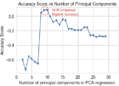
Dimensionality Reduction for PCA. Fig. 15 shows that the PCA model reduces the dimensionality from 71 inputs to 10 principal components (PCs) that explain over 90% of the variance of the model for both UX1 3 and 5-days forward. In the second graph, the number of PCs is chosen at the lowest MSE, which is 10. Similarly, in Appendix 10, maximum accuracy is shown to be optimized at 10 PCs.

Fig. 15. PCA Reduction to 10 Principal Components (PCs) with Explained Variance over 90% for 1-mth VIX Futures (UX1) 3 and 5-days Fwd. In addition, the second graph shows that with 10 PCs the MSE is minimized for both 3 and 5-days Fwd. (Jul 2006 to Jun 2015)

Fig. 16. PCA Scatter Plot of Training & Test Actual vs. Estimated for 1-mth VIX Futures (UX1) 3-days Forward and Error Histogram of Estimated Test vs. Actual UX_3D_FWD (Jul 2006 to Jun 2015 for Train & Jun 2015 to Jun 2018 for Test)

Quality Assessment of Results for PCA. Fig. 16 shows the PCA scatterplot of the output for the training versus test actual and estimated values as well as 1 to 1 plot of the perfect output for the training dataset as a benchmark for UX1 3-days forward. The scatterplots show generally a linear relationship for both the test and training

(20)

estimates with a slightly tighter variance in the test estimates. In addition, Fig. 15 shows the PCA error histogram of the actual versus estimated for the test data sets for UX1 3 days forward. The test data error histograms are still left skewed.

Appendix 10 contains the complete test and training data graphs and tables for the PCA analysis for 1-mth VIX futures both 3 and 5 days forward.

Table 6 shows a summary of results for both our 10-split cross validation and the 75%/25% train/test split. Using 10-split cross validation, the MSE of the test data is slightly higher and the variance explained (R2_{) of the test is higher than the} traditional split. For the output of our accuracy matrix, see Appendix 10.

Table 6. Some Quality Assessment Results of PCA Model

Output Inputs Traditional 75%/25% Train/Test Split 10-Split CV R2_train _R2_test_MSE_train _MSE_test _ρ(train)* _ρ(test)* _R2_test _MSE_test 3D Fwd. 10 0.86 0.22 11.80 19.38 0.93 0.70 0.339 29.10 5D Fwd. 10 0.84 0.03 13.77 21.93 0.92 0.61 0.334 30.39 *ρ(train) is the correlation of the actual to the estimated training data set (in-sample). ρ(test) is the correlation of the actual to the estimated test data set (out-sample)

4.3 Common Model: Univariate Auto-Regressive Integrated Moving Average (ARIMA)

Inputs: Univariate Autoregressive Integrated Moving Average (ARIMA) is a different model with only 1 input, the response variable. The response variable is used to forecast the future response.

Fig. 17. ARIMA Scatter Plot of Test Actual vs. Estimated for 1-mth VIX Futures (UX1) 3-days Forward (Jun 2015 to Jun 2018 for Test)

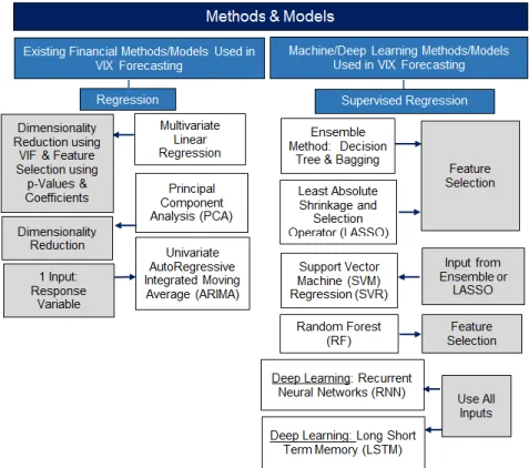
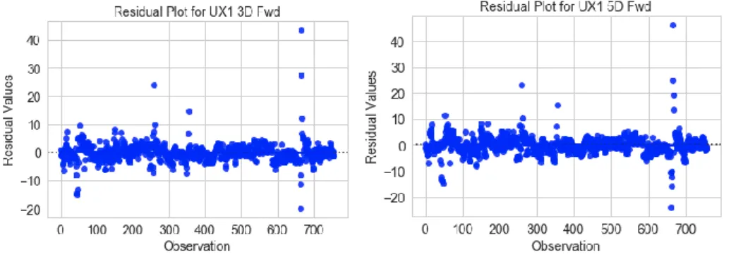
For this to occur, there has to be autocorrelation in the variable as was shown in section 2.3 earlier in this paper. In section 2.3, the optimal lag for an ARIMA model was 1. Fig. 17 shows the actual versus the estimated 1-mth VIX 3-days forward for the ARIMA model. Fig. 18 shows the residuals which jump during high volatility moves; otherwise, variance is generally more consistent within a range for both UX1

(21)

3 and 5-days forward. Appendix 11 contains the complete test and training data graphs and tables for the ARIMA analysis for 1-mth VIX futures both 3 and 5 days forward.

Fig. 18. ARIMA Residual Plot of Test Data for 1-mth VIX Futures (UX1) 3 and 5-days Forward (Jun 2015 to Jun 2018 for Test)

Table 7 is shows that the ARIMA model has a good explained variance and low MSE. However, it can be difficult to add more variables to the ARIMA model (multivariate ARIMA) compared to RNN and LSTM. In addition, ARIMA can have trouble forecasting inflection points based solely on the prior response level.

Table 7. Some Quality Assessment Results of ARIMA Model Traditional 75%/25% Train/Test Split

Output Forecasted

Inputs R2_test_MSE_test 3D Fwd. 1 0.52 6.44 5D Fwd. 1 0.36 8.63

4.4 Machine Learning: Ensemble Method

The ensemble method incorporates the error term from the forecast of the prior day. In our implementation, the data was first normalized, and then the ensemble method was used with a linear regression method, incorporating the prior error term into the forecast. In our case the error term cannot be known until 3 or 5 days from the closing price for each day in the dataset.

Feature Selection for Ensemble: Fig. 19 shows the top 15 predictors (input variables) plus 1 error term from our ensemble model for UX1 3 and 5 days forward. The top 15 predictors explain a majority of the variance and reduces the MSE to a minimum level.

Bootstrapping refers to any test or metric that relies on random sampling with replacement. It falls in to the broader class of resampling methods. It generates a new dataset for each ensemble member by bootstrapping, i.e. sample N items with

Residuals jump during high vol; otherwise, variance fairly constant

Residuals jump during high vol; otherwise variance fairly constant

(22)

replacement from the original N. Bagging uses bootstrap sampling to obtain the data subsets for training the base learners. In addition, bagging uses averaging for regression.

In addition, ensemble usually adds an error term as an input to forecast the response variables after finding the optimal model. First, the error term for our dataset has to be moved forward 3 or 5 days because it is not known until the actual UX1 level 3 or 5-days forward is realized. Second, the error term is also predicted as a third response variable, which is not moved forward, since it is used as our training data response variable. The added error term improves the estimate. The predicted error term is added to the predicted UX1 levels 3 or 5-day forward using out data set with the error term as an input moved forward. In our case, ensemble chose decision trees as the best estimator.

Fig. 19. Ensemble Top 15 Predictors plus 1 Error Term that Provide Optimal Results for UX1 3 and 5D Forward (Jul 2006 to Jun 2015)

Top Predictors (Inputs): UX6_HILO, VVIX, VVIX_HILO, UX4MUX2, UX3MUX2, UX7MUX2, UX7MUX4, UX6MUX2, M6_200_100, M3_150_100, M2_120_80, M3_100_80, M2_200_100, M3_200_100, M1_150_100 and TRAIN_ERR (training error term). See Appendix 3 for descriptions of each variable. The set of variables for 3 and 5-days forward is the same.

Optimization of Hyper-Parameters for BaggingRegressor Function in Python: The parameters are optimized by iterating using ParameterGrid for base estimator, maximum sample, maximum feature, and bootstrap (on or off) and bootstrap features (on or off). In addition, the base estimator iterates over estimators DecisionTree, DummyRegressor, DecisionTreeRegressor, KNeighborRegressor and SVR. The optimal hyper-parameters using the best estimator (DecisionTree) are all the samples (1.0), all the features (1.0), bootstrapping (True) and bootstrap features (False). Quality Assessment of Results for Ensemble Incorporating Error Term: Fig. 20 shows the ensemble scatterplot of the output for the training versus test actual and estimated values as well as 1 to 1 plot of the perfect output for the training dataset as a benchmark for UX1 both 3 and 5 days forward. The scatterplots show an estimate with increasing variance as volatility increases compared to the 1 to 1 plot line for the test estimate while the training estimates shows better results and a tighter variance versus the 1 to 1 plot. Appendix 12 contains the complete test and training data

(23)

graphs and tables for the ensemble analysis for 1-mth VIX futures both 3 and 5 days forward.

Fig. 20. Ensemble Scatter Plot of Training & Test Actual vs. Estimated for 1-mth VIX Futures 3 and 5 days Forward

Table 8 shows a summary of results for both our 10-split cross validation and the 75%/25% train/test split. The ensemble decision tree (DT) using bagging regression with a prior error term (DT with error term) shows great results for our traditional 75% train/25% test data split with a high explained variance (R2_{) and low MSE but} the 10-split time series cross validation shows a higher MSE and much lower explained variance. The higher MSE for the 10-split cross validation is due to much less accurate predictions of inflection points, such as the mortgage crisis of 2008 (the Great Recession) and the European debt crisis (the PIGS). Additionally, our model attempts to capture these inflection points. Similarly, for UX1 5D forward, the predictions or estimates also have good results for our 75% training /25% test data but worse results using our 10-split time series cross validation. For the output of our accuracy matrix, see Appendix 12. Once again, the accuracy matrix is good for the traditional split UX1 3D forward but less accurate for the traditional split of UX1 5D forward.

Table 8. Some Quality Assessment Results of Ensemble Decision Tree using Bagging Regression with Prior Error Term

Output Inputs Traditional 75%/25% Train/Test Split 10-Split CV R2_train _R2_test_MSE_train _MSE_test _ρ(train)* _ρ(test)* _R2_test _MSE_test 3D Fwd. 16 0.98 0.40 1.58 9.11 0.99 0.80 0.05 43.49 5D Fwd. 16 0.99 0.26 0.14 15.57 0.99 0.59 -0.19 49.45 *ρ(train) is the correlation of the actual to the estimated training data set (in-sample). ρ(test) is the correlation of the actual to the estimated test data set (out-sample)

4.5 Machine Learning: Least Absolute Shrinkage and Selection Operator (LASSO)

For the Least Absolute Shrinkage and Selection Operator (LASSO) method, the data was first normalized and then then the linear model for LASSO was run in python

(24)

(‘linear_model.Lasso’). The LASSO performs both variable selection and regularization in order to enhance the prediction accuracy and interpretability of the statistical model.

Dimensionality Reduction for LASSO: For UX1 3D forward, LASSO reduced the input dimensions from 71 to 16 and for 5D forward, from 71 to 15. LASSO reduces the number of predictors, identifies important predictors, selects among redundant predictors and produces shrinkage estimates with lower predictive errors than ordinary least squares. The selected input variables of LASSO are then used to select the final inputs of the linear regression model.

Top Predictors (Inputs): UX1 3D forward has 16 inputs and UX1 5D Forward has 15 inputs with a 94% overlap. LASSO for UX1 3D forward has the following inputs: UX7MUX2, UX8MUX2, VVIX, VVIX_HILO, M1_120_80, M1_150_100, M1_200_100, M2_120_80, M2_100_80, M2_200_100, M3_120_80, M3_100_80, M3_200_100, M6_120_80, M6_100_80, M12_200_100. LASSO for UX1 5D forward has all the same input excluding one, M2_200_100. See Appendix 3 for descriptions of each variable.

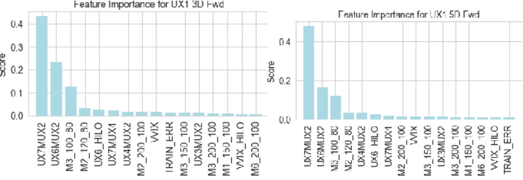
Optimization of Hyper-Parameters for LASSO: Alpha is the elasticity factor that controls the balance between lasso and ridge penalties. Our analysis uses a higher alpha of 0.95 (testing a range between 1.0 and 0) to reduce the MSE for both UX1 3 and 5-days forward shown in Fig. 21. The objective function is following:

min ww[[ (1 / (2 * n samples)) * ||X-y||22 + α * ||w||1 ] (1)6

The lasso estimate thus solves the minimization of the least-squares penalty with

α*||w||1 added, where α is a constant and ||w||1 is the L1-norm of the parameter vector. The higher the alpha value, more restriction on the coefficients; while the lower the alpha, more generalization and coefficients are barely restricted (at zero, it becomes a simple linear regression). The maximum number of iterations does not seem to matter so we set it at 10k.

Fig. 21. LASSO Alphas versus MSE for test data for both UX1 3 and 5-days forward (Jun 2015 to Jun 2018 )

6 _{http://scikit-learn.org/stable/modules/linear_model.html}

alpha = 0.95 alpha = 0.95

(25)

Quality Assessment of Results for LASSO: Fig. 22 shows the LASSO scatterplot of the output for the training versus test actual and estimated values as well as 1 to 1 plot of the perfect output for the training dataset as a benchmark for both UX1 3 days forward. The scatterplots show generally a linear relationship for both the test and training estimates for 3 days forward. In addition, Fig. 22 shows the LASSO error histogram of the actual versus estimated for the test data sets for UX1 for 3 days forward. The test data error histograms are slightly right skewed but more normal than other models so far, indicating a slightly better fit using LASSO. Similar results exist for 5-days forward as shown in Fig. 23. Appendix 13 contains the complete test and training data graphs and tables for the LASSO analysis for 1-mth VIX futures both 3 and 5 days forward.

Fig. 22. LASSO Scatter Plot of Training & Test Actual vs. Estimated for 1-mth VIX Futures 3-days Forward and Error Histogram of Estimated Test vs. Actual UX_3D_FWD (Jul 2006 to Jun 2015 for Train & Jun 2015 to Jun 2018 for Test)

Fig. 23. LASSO Scatter Plot of Training & Test Actual vs. Estimated for 1-mth VIX Futures 5-days Forward and Error Histogram of Estimated Test vs. Actual UX_5D_FWD (Jul 2006 to Jun 2015 for Train & Jun 2015 to Jun 2018 for Test)

Table 9 shows a summary of results for both our 10-split cross validation and the 75%/25% train/test split. Using 10-split cross validation, the MSE of the test data is higher and the R2_{of the test is higher than the traditional split. The results so far}

(26)

look very good compared to the models analyzed so far except the MSE for our 10-Split cross-validation is higher. For the output of our accuracy matrix, see Appendix 13.

Table 9. Some Quality Assessment Results of LASSO

Output Inputs Traditional 75%/25% Train/Test Split 10-Split CV R2

train R2test MSEtrain MSEtest ρ(train)* ρ(test)* R2test MSEtest 3D Fwd. 16 0.83 0.39 14.21 16.16 0.91 0.72 0.33 42.75 5D Fwd. 15 0.81 0.22 16.09 18.54 0.90 0.62 0.32 53.64 *ρ(train) is the correlation of the actual to the estimated training data set (in-sample). ρ(test) is the correlation of the actual to the estimated test data set (out-sample)

4.6 Machine Learning: Support Vector Regression (SVR)

For the Support Vector Machine Regression (SVR) method, the data was first normalized.

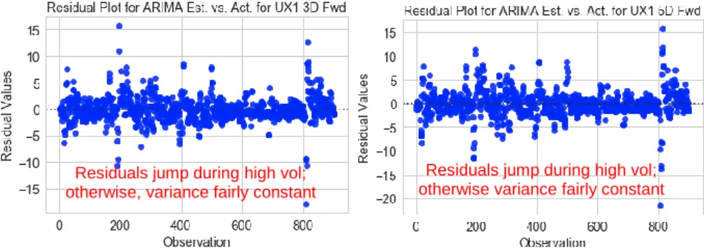
Dimensionality Reduction for SVR: For SVR, the top features from the ensemble and LASSO model are used as optimized inputs. The inputs from ensemble worked the best and ensemble reduced dimensionality to 15 inputs.

Top Predictors (Inputs): UX6_HILO, VVIX, VVIX_HILO, UX4MUX2, UX3MUX2, UX7MUX2, UX7MUX4, UX6MUX2, M6_200_100, M3_150_100, M2_120_80, M3_100_80, M2_200_100, M3_200_100, M1_150_100. See Appendix 3 for descriptions of each variable. The input variables for 3 and 5-days forward are the same.

Optimization of Hyper-Parameters for SVR: The parameters optimized are the following: the better kernel is linear; penalty factor (c) is 0.1; max iterations = 10k; and tolerance is 0.0001. The better kernel is linear but the sigmoid, rbf, and poly kernels were tested as well. The penalty factor of the error term was moved to 0.1 with the better results, after testing a range from 1.0 to 0.01. For large values of (c), the optimization will choose a smaller-margin hyperplane if that hyperplane does a better job of getting all the training points classified correctly. Conversely, a very small value of (c) will cause the optimizer to look for a larger-margin separating hyperplane, even if that hyperplane misclassifies more points. A hard limit of 10K for number of iterations was set. The criteria of tolerance for stopping was made tighter from 0.001 to 0.0001 to achieve better results.

Quality Assessment of Results for SVR: Fig. 24 shows the SVR scatterplot of the output for the training versus test actual and estimated values as well as 1 to 1 plot of the perfect output for the training dataset as a benchmark for both UX1 3 days forward. The scatterplots show generally a linear relationship for both the test and training estimates for 3 days forward; however, there are a few data points with large variances from the 1 to 1 line. In addition, Fig. 24 shows the SVR error histogram of the actual versus estimated for the test data sets for UX1 for 3 days forward. The test data error histograms are only slightly left skewed but still closer to normal, indicating a better fit. Similar results exist for 5-days forward as shown in Fig. 25. Appendix 13 contains the complete test and training data graphs and tables for the SVR analysis for 1-mth VIX futures both 3 and 5 days forward.

(27)

Fig. 24. SVR Scatter Plot of Training & Test Actual vs. Estimated for 1-mth VIX Futures 3-days Forward and Error Histogram of Estimated Test vs. Actual UX_3D_FWD (Jul 2006 to Jun 2015 for Train & Jun 2015 to Jun 2018 for Test)

Fig. 25. SVR Scatter Plot of Training & Test Actual vs. Estimated for 1-mth VIX Futures 5-days Forward and Error Histogram of Estimated Test vs. Actual UX_5D_FWD (Jul 2006 to Jun 2015 for Train & Jun 2015 to Jun 2018 for Test)

Table 10 shows a summary of results for both our 10-split cross validation and the 75%/25% train/test split. Using 10-split cross validation, the MSE of the test data is higher and the R2_{of the test is higher than the traditional split. The results so far} look very good compared to the models analyzed so far except the MSE for our 10-Split cross-validation is high. For the output of our accuracy matrix, see Appendix 14.

Table 10. Some Quality Assessment Results of SVR

(28)

4.7 Machine Learning: Recurrent Neural Networks (RNN)

In traditional neural networks, all inputs and outputs are independent with no memory of prior levels. However, RNNs and LSTMs have “memory” to capture information

about what is already calculated in the prior time series. Three of the many factors to optimize in neural networks (RNN and LSTM) are number of epochs, batch size and number of iterations.

Table 11 defines these inputs to the model. For batch size, 44 business days (2-mth) turns out to be optimal for RNN and 66 business days (3-mths), for LSTM. This makes sense since generally markets have shorter memories.

Table 11. Definition of Three Inputs in NN model for RNN and LSTM

Input Variable Definition

1 Epoch 1 forward & 1 backward pass of all the training data Batch Size total number of data samples in a single batch for one

forward and backward pass

Iterations the number of batches or passes needed to complete 1 epoch 1 Pass 1one forward and one backward pass

Inputs: All 71 inputs are utilized for both response variables

Optimization of Hyper-Parameters for RNN: The parameters optimized are the following using GridSearchCV in Python: optimizer is Adam; initialization mode is uniform; loss function is mean squared error; activation function is relu; number of neurons for each layer is 150; metric output is accuracy; epochs is 300; batch size is 44 (approximately two months of data); dropout rate is 0 and learning rate is 0.001. A smaller number of layers and neurons used due to our smaller data set of only 71 inputs of 3009 entries each. The number of hidden layers is 1 with 10 neurons with one output layer for our response variable. For the traditional 75% training / 25% test split, the training input size is 2256 by 71.

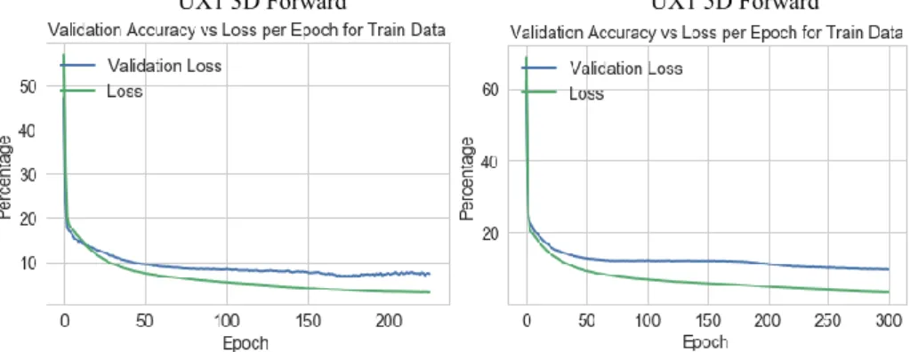
Quality Assessment of Results for RNN: Fig. 26 shows the validation accuracy versus loss per epoch for the training data, which shows that there is little improvement after 200 epochs for UX1 3 and 5-days forward. The lower the loss, the better a model (unless the model has over-fitted to the training data).

(29)

UX1 3D Forward UX1 5D Forward

Fig. 26. Validation Accuracy versus Loss per Epoch for Training Data for both 1-mth VIX Futures 3 and 5-Days Forward

The loss is calculated on training and validation. The interpretation of the loss is how well the model is doing for these two sets. Unlike accuracy, loss is not a percentage. It is a summation of the errors made for each example in training or validation sets.

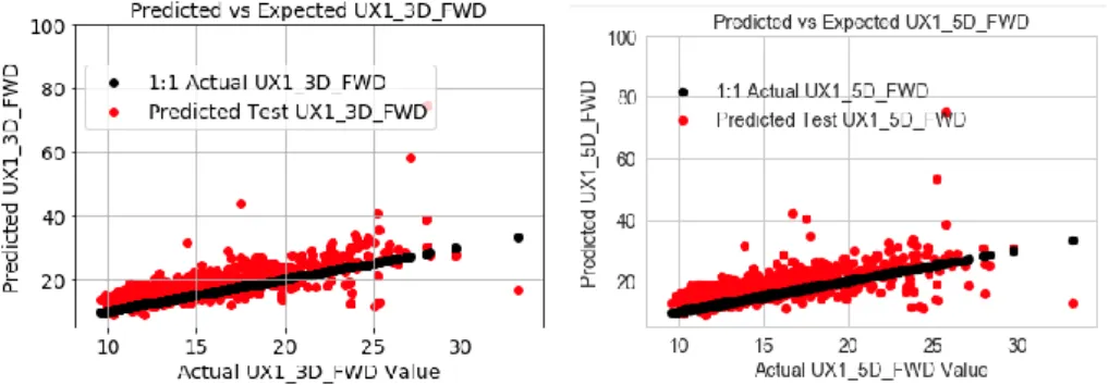
Fig. 27 shows the RNN scatterplot of the output for the training versus test actual and estimated values as well as 1 to 1 plot of the perfect output for the training dataset as a benchmark for both UX1 3 and 5-days forward. The scatterplots show generally a linear relationship for both the test and training estimates for 3 days forward. In addition, Fig. 27 shows the RNN error histogram of the actual versus estimated for the test data sets for UX1 for 3 days forward. The test data error histograms are closer to a normal distribution, indicating a better fit and the variance of the test estimated are closer to the 1 to 1 line, indicating less variance. Similar results exist for 5-days forward as shown in Fig. 28. Appendix 15 contains the complete test and training data graphs and tables for the RNN analysis for 1-mth VIX futures both 3 and 5 days forward.

Fig. 27. RNN Scatter Plot of Training & Test Actual vs. Estimated for 1-mth VIX Futures 3-days Forward and Error Histogram of Estimated Test vs. Actual UX_3D_FWD (Jul 2006 to Jun 2015 for Train & Jun 2015 to Jun 2018 for Test)

(30)

Fig. 28. RNN Scatter Plot of Training & Test Actual vs. Estimated for 1-mth VIX Futures 5-days Forward and Error Histogram of Estimated Test vs. Actual UX_5D_FWD (Jul 2006 to Jun 2015 for Train & Jun 2015 to Jun 2018 for Test)

Table 12 shows a summary of results for both our 10-split cross validation and the 75%/25% train/test split. Using 10-split cross validation, the MSE of the test data is higher and the R2_{of the test is about the same as the traditional split. Overall for} both the traditional and 10-split cross validation, the results are very good compared to the models analyzed so far with higher variance explained (R2_{) and lower MSE.} For the output of our accuracy matrix, see Appendix 15.

Table 12. Some Quality Assessment Results of RNN

4.8 Machine Learning: Long Short-Term Memory (LSTM)

Long Short-Term Memory (LSTM) is similar to RNN but can have a longer memory of prior forecasts. Having multiple layers (a deeper network) makes your network more eager to recognize certain aspects of input data; however, our data is not as complex and only one hidden layer seems to improve performance over other models. Inputs: All 71 inputs are utilized for both response variables.

Optimization of Hyper-Parameters for LSTM: The parameters optimized are the following using GridSearchCV in Python: optimizer is Adam; initialization mode is uniform; loss function is mean squared error; activation function is relu; number of neurons for each layer is 150; metric output is accuracy; epochs is 300, batch size is 66 (approximately three months of data); refit data is True; dropout rate is 0; and learning rate is 0.001. A smaller number of layers and neurons used due to our smaller data set of only 71 inputs of 3009 entries each. The number of hidden layers is 1 with 10 neurons with one output layer for our response variable. For the traditional 75% training / 25% test split, the input size is 2256 by 71.

(31)

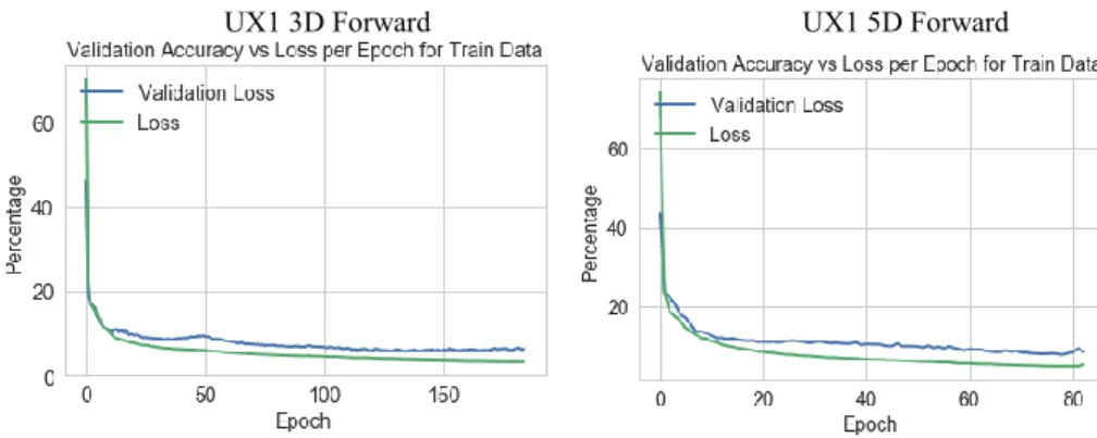
Quality Assessment of Results for LSTM: Fig. 29 shows the validation accuracy versus loss per epoch for the training data, which shows that there is little improvement after 200 epochs for UX1 3 and 5-days forward. The lower the loss, the better a model (unless the model has over-fitted to the training data). The loss is calculated on training and validation and its interpretation is how well the model is doing for these two sets. Unlike accuracy, loss is not a percentage. It is a summation of the errors made for each example in training or validation sets.

UX1 3D Forward UX1 5D Forward

Fig. 29. Validation Accuracy versus Loss per Epoch for Training Data for both 1-mth VIX Futures 3 and 5-Days Forward

Fig. 30 shows the LSTM scatterplot of the output for the training versus test actual and estimated values as well as 1 to 1 plot of the perfect output for the training dataset as a benchmark for both UX1 3 days forward. The scatterplots show generally a linear relationship for both the test and training estimates for 3 days forward. In addition, Fig. 30 shows the LSTM error histogram of the actual versus estimated for the test data sets for UX1 for 3 days forward. The test data error histogram has a left skew unlike RNN. Similar results exist for 5-days forward as shown in Fig. 31. Appendix 16 contains the complete test and training data graphs and tables for the LSTM analysis for 1-mth VIX futures both 3 and 5 days forward.

(32)

Fig. 30. LSTM Scatter Plot of Training & Test Actual vs. Estimated for 1-mth VIX Futures 3-days Forward and Error Histogram of Estimated Test vs. Actual UX_3D_FWD (Jul 2006 to Jun 2015 for Train & Jun 2015 to Jun 2018 for Test)

Fig. 31. LSTM Scatter Plot of Training & Test Actual vs. Estimated for 1-mth VIX Futures 5-days Forward and Error Histogram of Estimated Test vs. Actual UX_5D_FWD (Jul 2006 to Jun 2015 for Train & Jun 2015 to Jun 2018 for Test)

Table 13 shows a summary of results for both our 10-split cross validation and the 75%/25% train/test split. Using 10-split cross validation, the MSE of the test data is higher and the R2_{of the test is about the same as the traditional split. Overall for} both the traditional and 10-split cross validation, the results are good compared to the models analyzed but still a slight left skew in the histogram and a bit more variance from the 1 to 1 line compared to RNN. The MSE is slightly higher for 10-split cross validation of the time series than for the traditional split. For the output of our accuracy matrix, see Appendix 16.

Table 13. Some Quality Assessment Results of LSTM

4.9 Machine Learning: Random Forest (RF)

Random Forest (RF) is an ensemble method that performs feature selection.

Top Features (Inputs): UX7MUX2, UX6MUX2, M3_100_80, UX5MUX2, UX6MUX3, M3_120_80, UX7MUX3, M2_120_80, M2_100_80, UX4MUX2, M2_200_100, UX7MUX4, UX2_HILO, and M12_200_100. See Appendix 3 for descriptions of each variable. See Appendix 3 for descriptions of each variable.

(33)

The top 14 input variables for 3 and 5-days forward are the same. And shown in Fig. 32.

Fig. 32. Top 14 Features Selected for 1-mth VIX Futures 3 and 5-Days Forward Optimization of Hyper-Parameters for RF: The parameters optimized are the following using GridSearchCV in Python: trees or estimators are 200, criterion is mean squared error, maximum depth has no limit, minimum leaf samples are 1, max features are auto, and bootstrap is True. Fig. 32 show the output of both 3 and 5-day feature selection using the top 15 factors to explain most of the variance.

Quality Assessment of Results for RF: Fig. 33 shows the RF scatterplot of the output for the training versus test actual and estimated values as well as 1 to 1 plot of the perfect output for the training dataset as a benchmark for both UX1 3 days forward. The scatter plots show a bias to low ranges in the training data estimate which actually works for our test data estimate. Since the VIX generally stays at lower volatility levels, it makes sense a majority of the trees would have a lower range. Decision trees tend to have high variance when they utilize different training and test sets of the same data, since they tend to overfit on training data. This can lead to poor performance on forecasting inflection points. Unfortunately, this limits the usage of decision trees in predictive modeling as seen in our results. In addition, Fig. 33 shows the RF error histogram of the actual versus estimated for the test data sets for UX1 for 3 days forward. The test data error histogram has a right skew. Similar results exist for 5-days forward as shown in Fig. 34 but for 5-days the error histogram has more of a normal distribution. Appendix 17 contains the complete test and training data graphs and tables for the RF analysis for 1-mth VIX futures both 3 and 5 days forward.

(34)

Fig. 33. RF Scatter Plot of Training & Test Actual vs. Estimated for 1-mth VIX Futures 3-days Forward and Error Histogram of Estimated Test vs. Actual UX_3D_FWD (Jul 2006 to Jun 2015 for Train & Jun 2015 to Jun 2018 for Test)

Fig. 34. RF Scatter Plot of Training & Test Actual vs. Estimated for 1-mth VIX Futures 5-days Forward and Error Histogram of Estimated Test vs. Actual UX_5D_FWD (Jul 2006 to Jun 2015 for Train & Jun 2015 to Jun 2018 for Test)

Table 14 shows a summary of results for both our 10-split cross validation and the 75%/25% train/test split. Using 10-split cross validation, the MSE of the test data is higher and the R2_{of the test is about the same as the traditional split. Overall for} both the traditional and 10-split cross validation, the results are good compared to the models analyzed except for the bias toward a lower volatility forecast. The MSE is slightly higher for 10-split cross validation of the time series than for the traditional split. RF has some of the best quality metrics (high accuracy, low MSE, etc.); however similar to ensemble, predicting training data is biased to lower volatility forecasts due to the overfit even using the 10-split CV. For the output of our accuracy matrix, see Appendix 17.

(35)

Table 14. Some Quality Assessment Results of RF

5 Analysis

In this section, the results of choosing the best model for each method are compared for 1-mth VIX futures 3 and 5-days forward. In addition, the accuracy matrix calculations are presented and analyzed.

5.1 Analysis of Forecast Results for 1-Mth VIX Futures 3-Days Forward Table 15 and 16 shows the result for the 1-mth VIX futures forecast 3 days forward across all models for both traditional 75% train/25% test split and cross-validation 10-split time series. The best first and second results for each column are highlighted in yellow. Across the multiple metrics, the machine/deep learning models RNN, LSTM, RF and the ensemble decision tree using bagging regressor with prior error term (Ensemble DT with Err. Term) have better quality assessment metrics compared to the other models. RNN has the best metrics for both the traditional 75% train/25% test split and the cross validation with 10 time series splits. Explained variance for the test data sets are generally low across most models. RF has great quality assessment, but it can be biased to lower volatility forecasts (see section 4.9). Similarly, the ensemble DT with error term (see section 4.4) shows great results for our traditional 75% train/25% test data split with a high explained variance (R2_{) and} low MSE but the 10-split time series cross validation shows a higher MSE and much lower explained variance, indicating potential overfitting using the traditional split. For RF and DT with error term, the higher MSE for the 10-split cross validation is due to much less accurate predictions of inflection points, such as the mortgage crisis of 2008 (the Great Recession) and the European debt crisis (the PIGS). Additionally, our model attempts to capture these inflection points.