Efficient Scheduling Algorithms for Wireless Resource Allocation and Virtualization in Wireless Networks

(1)

Scholarship@Western

Electronic Thesis and Dissertation Repository

11-27-2015 12:00 AM

Efficient Scheduling Algorithms for Wireless Resource Allocation

and Virtualization in Wireless Networks

Mohamad Kalil

The University of Western Ontario

Supervisor Abdallah Shami

The University of Western Ontario

Graduate Program in Electrical and Computer Engineering

A thesis submitted in partial fulfillment of the requirements for the degree in Doctor of Philosophy

Follow this and additional works at: https://ir.lib.uwo.ca/etd Part of the Digital Communications and Networking Commons

Recommended Citation Recommended Citation

Kalil, Mohamad, "Efficient Scheduling Algorithms for Wireless Resource Allocation and Virtualization in Wireless Networks" (2015). Electronic Thesis and Dissertation Repository. 3445.

https://ir.lib.uwo.ca/etd/3445

This Dissertation/Thesis is brought to you for free and open access by Scholarship@Western. It has been accepted for inclusion in Electronic Thesis and Dissertation Repository by an authorized administrator of

(2)

Resource Allocation and Virtualization in

Wireless Networks

(Thesis format: Monograph)

by

Mohamad Kalil

Graduate Program in

Electrical and Computer Engineering

A thesis submitted in partial fulfillment of the requirements for the degree of

Doctor of Philosophy

School of Graduate and Postdoctoral Studies The University of Western Ontario

London, Ontario, Canada

c

(3)

The continuing growth in demand for better mobile broadband experiences has motivated rapid development of radio-access technologies to support high data rates and improve quality of service (QoS) and quality of experience (QoE) for mobile users. However, the modern radio-access technologies pose new challenges to mobile network operators (MNO) and wireless device designers such as reducing the total cost of ownership while supporting high data throughput per user, and extending battery life-per-charge of the mo-bile devices. In this thesis, a variety of optimization techniques aimed at providing innova-tive solutions for such challenges are explored.

The thesis is divided into two parts. In the first part, the challenge of extending battery life-per-charge is addressed. Optimal and suboptimal power-efficient schedulers that minimize the total transmit power and meet the QoS requirements of the users are presented. The second outlines the benefits and challenges of deploying wireless resource virtualization (WRV) concept as a promising solution for satisfying the growing demand for mobile data and reducing capital and operational costs. First, a WRV framework is proposed for single cell zone that is able to centralize and share the spectrum resources between multiple MNOs. Consequently, several WRV frameworks are proposed, which virtualize the spectrum resource of the entire network for cloud radio access network (C-RAN)- one of the front runners for the next generation network architecture.

The main contributions of this thesis are in designing optimal and suboptimal solu-tions for the aforementioned challenges. In most cases, the optimal solusolu-tions suffer from high complexity, and therefore low-complexity suboptimal solutions are provided for prac-tical systems. The optimal solutions are used as benchmarks for evaluating the suboptimal solutions. The results prove that the proposed solutions effectively contribute in addressing the challenges caused by the demand for high data rates and power transmission in mobile networks.

Keywords: Power Minimization, QoS, LTE, Packet Scheduling, Uplink, Virtualiza-tion, C-RAN, Resource Sharing

(4)

I would like to express my sincere gratitude to my supervisor, Prof. Abdallah Shami, for the immeasurable amount of support, guidance, and personal and professional advices he has provided me while pursuing this degree. I could not imagine having a better supervisor for my PhD study. I appreciate all his contributions of time, ideas and support to make my PhD experience productive, successful and enjoyable. Thank you for motivating me along the way and for being the go-to person whenever I faced problems or felt down. I knew I could always turn to him when my depleted motivation needed recharging.

My sincere gratitude goes to my co-supervisor Dr. Arafat Al-Dweik for his continuous help and support in all stages of my PhD study. Without his involvement, this work will not have been possible. His encouragement, kindness, brilliant comments and insightful suggestions, and his prompt responses to my questions will always be remembered. I would like to thank my examiners: Dr. Serguei Primak, Dr. Lian Zhao, Dr. Aleksander Essex, and Dr. Michael Bauer for taking the time to review and examine my thesis, and for their insightful comments and suggestions.

I would also like to thank my Master’s thesis supervisor, Dr. Mohammad Banat, for help-ing me to begin my research journey. I would like to thank Dr. Ibrahim M. Ghareeb and Dr. Redha Radaydeh, who taught me the first courses in wireless communication and in-troduced me to the area.

Special thanks go to my colleagues and friends at Western university who made my PhD years a joyful and memorable experience. For most, a BIG thanks to Mohamed Abu Sharkh who experienced all of the ups and downs of my research, and to Fuad Shamieh who was always there for me and ready to help. Also, I would like to extend my thanks to my friends: Oscar Filio, Karim Hammad, Aidin Reyhani, Dan Wallace, , Manar Jammal, Has-san Hawilo, Bradley de Vlugt, Elena Uchiteleva, Abdallah Moubayed, Khaled Alhazmi, Emad Aqeeli, Mohamed Hussein, Maysam Mirahmadi, Khalim Meerja, Siamack Ghadimi, M. Ajmal Khan, Eric Southern, Peng Hao, Mohamed Youssef, Abdulfattah Noorwali, Mo-hammad Noor Injadat, Fadi Salo, Anas Saci, Marco Luccini, Anas Ibrahim, Jay Nadeau, and Kevin Mi.

To my friends scattered around the world, thank you for your well-wishes, phone calls, e-mails, and being there whenever I needed a friend. For most, I would like to thank Yazan Al-Badarneh, Khair Al Shamaileh, Majdi Ababneh, Alaeddin Bani Milhim, Ali

(5)

Bani Amer, Yousef Mashaala, Bashar Alwadyan, Malek Khudirat, Qutaiba Al-Hazaime, Mohamad Abu Hani, Hasan Thiabat, and Ahmad Al-Sharoa.

A warm thanks goes to Madeleine and Carl, whom I lived with for almost 3 years, for being warm, kind, and a second family for me.

And most importantly, I am deeply and forever indebted to my family. You are the great-est source of love, encouragement, and inspiration. In particular, this project is dedicated to them with my sincerest thanks and appreciation to my father, God bless his soul, who passed away last may, and to my mother for their love, support and encouragement through-out my entire life, and for all of the sacrifices they have made on my behalf. Withthrough-out them I would have been totally lost and never took a step ahead.

My sincere gratitude goes to my sisters Maysa, Mayada, Maram, and Marwa, and my brothers, Motaz and Mones, as well as to my grandmothers, grandfathers, father-in-law, mother-in-law, brothers-in-law, sister-in-law, aunts, uncles, and cousins for their love and support, and for being proud of me.

Last but not least, a heartfelt thanks to my wife Tasneem for her continued support, love, and for being my best friend and great companion who helped me get through the unex-pected troubles of research in the most positive way. Words cannot describe how lucky I am to have you in my life.

(6)

(7)

Abstract . . . ii

Acknowledgements . . . iii

Dedication . . . v

Table of Contents . . . vi

List of Tables . . . ix

List of Figures . . . x

Acronyms . . . xii

1 Introduction . . . 1

1.1 Thesis Outline and Contributions . . . 2

1.2 Contributions of the Thesis . . . 3

1.2.1 Contributions of Chapter 2 . . . 3

2 QoS-Aware Power-Efficient Scheduler for LTE Uplink . . . 6

2.1 Introduction . . . 6

2.2 Related Work . . . 7

2.3 System Model . . . 9

2.3.1 LTE QoS and Buffer Status Reports (BSRs) . . . 13

2.3.2 Uplink Data Transmission Procedure . . . 15

2.3.3 Delay Analysis . . . 15

2.4 System Constraints and Objective . . . 18

2.5 BIP Formulation . . . 21

2.5.1 Binary Integer Programming . . . 24

2.5.2 Complexity of BIP . . . 26

2.6 Iterative Algorithm . . . 26

2.6.1 Complexity of the Iterative Algorithm . . . 27

(8)

2.8 Intra-User Scheduling . . . 30

2.9 Numerical Results . . . 30

2.9.1 Experiment 1: Two Users with Identical Conditions . . . 32

2.9.2 Experiment 2: Two Users with Identical Conditions but Different ACG . . . 33

2.9.3 Experiment 3: The Iterative Algorithm Evaluation . . . 34

2.10 Chapter Summary . . . 41

3 Low-Complexity Power-Efficient Schedulers for LTE Uplink with Delay-Sensitive Traffic . . . 42

3.1 Introduction . . . 42

3.2 System Model Description and Assumptions . . . 44

3.3 Allocation Constraints and Problem Definition . . . 50

3.3.1 Delay Constraint . . . 50

3.3.2 System Constraints . . . 51

3.3.3 Problem Definition . . . 52

3.4 Optimal Offline Scheduling . . . 53

3.5 Sub-Optimal Power-Efficient Schedulers . . . 59

3.5.1 Maximum Transmit Power Controlling (MTPC) Scheduler . . . 60

3.5.2 Bit per Watt Controlling (BWC) Scheduler . . . 63

3.5.3 Complexity of the Heuristic Algorithms . . . 64

3.5.4 The Controllers . . . 64

3.6 Simulation Results . . . 65

3.6.1 Large-Scale Scenario . . . 68

4 Wireless Resource Virtualization: Opportunities, Challenges, and Solutions . 76 4.1 Introduction . . . 76

4.2 Main Benefits of WRV . . . 78

4.2.1 Economic Sharing of Investment and Cost Reduction . . . 78

4.2.2 Collaborative Business Models . . . 79

4.2.3 Environmental Benefits . . . 79

4.3 Operational and Business Challenges of WRV Deployment . . . 80

4.3.1 The Risk of Market Share Loss and Anti-Competitive Practices . . 80

4.3.2 Independence of Services with RAN-Sharing . . . 80

4.4 Scope of Virtualization and Depth of Sharing . . . 80

4.4.1 Passive Sharing . . . 81

4.4.2 Active Sharing . . . 82

4.5 Efficient Fair Low-Complexity Scheduler for WRV . . . 85

4.5.1 System and Channel models . . . 86

4.5.2 Problem Formulation . . . 87

4.5.3 Computing the Optimal Weights for MNOs . . . 90

(9)

4.5.4 Numerical Results . . . 92

5 Wireless Resources Virtualization for Cloud Radio Access Networks (C-RAN) 96 5.1 Introduction . . . 96

5.2 Related work . . . 98

5.3 System and Sharing Models . . . 101

5.3.1 Resource Blocks Sharing Model . . . 103

5.4 Problem Formulation . . . 104

5.4.1 Special Case: Backlogged Traffic Model . . . 106

5.4.2 Radio Resource Scheduling Polices . . . 107

5.4.3 Complexity of Optimal Solution . . . 107

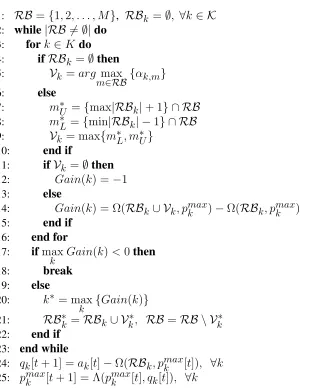
5.5 Low-Complexity Solutions . . . 108

5.5.1 The Complexity of the Heuristic Algorithm . . . 113

5.6 Simulation Model and Numerical Results . . . 113

5.6.1 Scenario 1: Backlogged Traffic Model . . . 114

5.6.2 Scenario 2: Dynamic Traffic Model . . . 117

6 Conclusion . . . 122

6.1 Thesis Summary . . . 122

6.2 Future Work . . . 124

6.2.1 Power-Efficient Schedulers for LTE-A Uplink . . . 124

6.2.2 Virtualization in Next Generation Radio Access Network . . . 125

6.2.3 Spectrum and Computing Resources Virtualization in C-RAN . . . 126

References . . . 127

Curriculum Vitae . . . 135

(10)

2.1 Summary of the most significant notation used in this chapter. . . 10

2.2 List of MCS indices [1] . . . 13

2.3 Iterative allocation . . . 28

2.4 Intra-user scheduling for userk . . . 30

2.5 Simulation default parameters . . . 31

2.6 Users’ data profile . . . 31

3.1 Summary of the most significant notation used in this chapter. . . 45

3.2 MTPC scheduler. . . 61

3.3 BWC scheduler. . . 62

3.4 MATP controller. . . 66

3.5 BPWR controller. . . 66

3.6 Parameter settings of the uplink LTE model. . . 67

3.7 Parameter settings of the large-scale scenario. . . 71

4.1 Summary of the most significant notation. . . 85

4.2 Iterative search method to find MNOs’ weights . . . 91

4.3 Number of iterations to converge . . . 93

5.1 Summary of the most significant notation. . . 102

5.2 Examples of different schedulers [2] . . . 108

5.3 Per RB optimal allocation algorithm . . . 111

5.4 Heuristic algorithm . . . 112

5.5 Normalized average running time of the BIP, heuristic, heuristic-RRH and static sharing solutions. . . 119

(11)

2.1 The structure of the LTE subframe. . . 11

2.2 BLER-SNR curves for all Table 2.2 MSC, from Index 1 (leftmost) to index 15 (rightmost) [3]. . . 12

2.3 An example of four bearers established for a user. . . 14

2.4 Uplink data transmission sequence. . . 16

2.5 Spectral efficiency versus SNR for the MCS that are shown in Table 2.2. . . 22

2.6 Extra weight demonstration forE_k = 200bits. . . 24

2.7 Experiment 1: Average transmitted power per user per TTI (Watt). . . 33

2.8 Experiment 1: Battery life comparison. . . 34

2.9 Experiment 1: Average queue length per bearer per user. . . 35

2.10 Experiment 1: Probability density function of the delay of the NGBR bear-ers at ACG=10. . . 35

2.11 Experiment 1: Average transmission rate per bearer per user. . . 36

2.12 Experiment 1: Time complexity comparison. . . 36

2.13 Experiment 2: Average transmitted power per TTI for user 1 (Watt). . . 37

2.14 Experiment 2: Average transmitted power per TTI for user 2 (Watt). . . 37

2.15 Experiment 2: Average queue length for the NGBR bearers in bits. . . 38

2.16 Experiment 2: Average transmission rate per bearer per user. . . 38

2.17 Experiment 3: Average transmitted power per user per TTI (Watt). . . 39

2.18 Experiment 3: Delay per bearer averaged on all users. . . 40

2.19 Experiment 3: Average transmission rate per bearer averaged on all users. . 40

3.1 A block diagram of a SC-FDMA system. . . 46

3.2 The structure of the LTE frame. . . 50

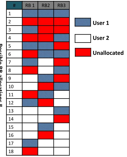
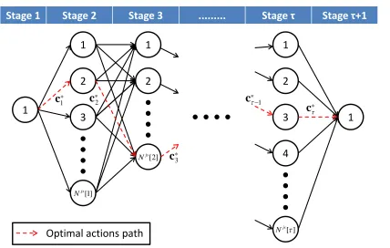
3.3 Contiguous allocations possible from three RBs. . . 52

3.4 An example of all possible RB allocations for a system consisting of three RBs shared between two users. . . 57

3.5 The components and the optimal action path of the DP problem. . . 58

3.6 Average transmit power per TTI. . . 68

3.7 Average queue length for UE1. . . 69

3.8 Average queue length for UE2. . . 69

3.9 Probability density function of the queue length for UE1 (average CNR=13 dB). . . 70

3.10 Probability density function of the queue length for UE2 (average CNR=13 dB). . . 70

(12)

3.11 Average transmit power per TTI for the large-scale scenario. . . 71

3.12 Average queue length for all users for the large-scale scenario. . . 72

3.13 Probability density function of the queue length for number of users 70. . . 72

3.14 Average transmit power for all users per TTI for differentl. . . 74

3.15 Average queue length for all users for differentl. . . 74

4.1 Base station virtualization. . . 77

4.2 Scope of virtualization. . . 81

4.3 LTE sharing configuration options. . . 83

4.4 The average aggregate throughput of MNOs as the number of users increases. 94 4.5 The average users’ throughput of MNOs as the number of users increases. . 94

4.6 Resource access probability analytical and simulation results. . . 95

5.1 Virtualized C-RAN shared between two MNOs. . . 99

5.2 Example of interference graphG= (V, E)of five weighted vertices (RRHs).110 5.3 Simulated network layout. For the first scenraio, only the red RRHs 1-6 are considered. For the second scenario, all RRHs are considered. . . 114

5.4 Average throughput per UE forT_sleep = 40%. . . 116

5.5 Average aggregate throughput per cell forT_sleep = 40%. . . 116

5.6 Average throughput per UE for MNO1’s users for different vales ofT_sleep. . 117

5.7 Average throughput per UE for MNO2’s users for different vales ofT_sleep. . 118

5.8 Average aggregate throughput of MNO1’s users. . . 119

5.9 Average head-of-line packet delay of MNO2’s users. . . 120

5.10 Average aggregate throughput of MNO1’s users. . . 120

(13)

3GPP 3rd Generation Partnership Project

ACG Average Channel Gain

APF Access Proportional Fairness

ARP Allocation and Retention Priority

AWGN Additive White Gaussian Noise

BIP Binary Integer Programming

BLER Block Error Rate

BPU Baseband Processing Unit

BPWR Bit per Watt Ratio

BS Base Stations

BSR Buffer Status Reporting

BWC Bit per Watt Controlling

CAPEX Capital Expenditure

CoMP Coordinated Multipoint

CPU Central Processing Unit

C-RAN Cloud Radio Access Network

DP Dynamic Programming

DU Data Unit

eNB Evolved Node-B

FFR Fractional Frequency Reuse

FR Frequency-Reuse

GBR Guaranteed Bit Rate

GPF Generalized Proportional Fair

GWCN Gateway Core Network

HetNet Heterogeneous Network

HoL Head-of-Line

(14)

ICI Intercell Interference

ICIC Intercell Interference Coordination

LSM Least Satisfied Mobile Network Operator

LTE Long Term Evolution

MAC Media Access Control

MATP Maximum Allowable Transmit Power

MCS Modulation And Coding Scheme

MDP Markov Decision Process

MIMO Multiple-Input Multiple-Output

M-LWDF Modified-Largest Weighted Delay First

MME Mobility Management Entity

MNO Mobile Network Operator

MOCN Multi-Operator Core Network

MT Maximum Throughput

Multi-RAT Multiple Radio Access Technology

MWIS Maximum Weighted Independent Set

NGBR Non Guaranteed Bit Rate

NGN Next Generation Network

OFDMA Orthogonal Frequency Division Multiple Access

OPEX Operating Expenditure

PAPR Lower Peak-To-Average Power Ratio

PDB Packet Delay Budget

PDF Probability Density Function

PDU MAC Protocol Data Units

PF Proportional Fair

PHY Physical Layer

QCI Quality of Service Class Identifier

QoS Quality of Service

RAP Resource Block Access Probabilities

RB Resource Block

RLC Radio Link Control

RRH Remote Radio Head

(15)

SC-FDMA Single Carrier Frequency Division Multiple Access

SINR Signal-to-Interference Plus Noise Ratio

SLA Service-Level Agreement

SNR Signal to Noise Ratio

SON Self-Organizing Network

SP Service Providers

SS Static Sharing

TTI Transmission Time Interval

UE User Equipment

vMNO Virtual Mobile Network Operator

WRV Wireless Resource Virtualization

(16)

Chapter 1 Introduction

The demand for mobile data is growing exponentially and mobile network operators (MNOs) are struggling more than ever to increase their capacity profitably. Mobile communication is becoming an essential need for individuals and businesses. The number of new mobile-connected devices added in 2014 reached almost half a billion, meaning the total number of mobile-connected devices exceeds the world’s population [4]. Mobile Internet-access is also visibly becoming affordable and available for a larger segment of the population. This leads to Internet usage levels we thought were once unreachable. A look at the Youtube statistics shows that more than 4 billion hours of video are watched on YouTube every month. Pressures on the infrastructure, service levels and performance have never been that high. The demand for mobile data does not stop there. Mobile data traffic forecasts estimate a 10-fold increase in global mobile data traffic between 2014 and 2019. This un-precedented penetration is accompanied by a major increase in mobile network connection speeds. For example, the average mobile network downstream speed increased 20 percent in 2014 [4].

(17)

transmission power, which makes power-efficient communication in uplink transmission an essential requirement for next-generation mobile networks.

Due to the large investments in network resources needed to support the surge in mobile data traffic, MNOs profits have not been growing at rate that the traffic volume level would indicate. In their continuous endeavors to tackle this issue, MNOs have become highly interested in cost-effective solutions in order to satisfy the high demand for mobile data. To maximize the average revenue per user, MNOs have to efficiently utilize the limited and highly expensive spectrum resources. A surprising fact here arises. Recent spectrum utilization measurements have shown that the bandwidth licensed to MNOs is mostly underutilized. According to a recent study by Nokia [7], only 20 percent of a radio access network’s full capacity is used at any given time with 80 percent being idle and waiting for peak hour demand. This motivates innovative solutions to efficiently use the limited spectrum resources and maximize profits.

1.1 Thesis Outline and Contributions

(18)

1.2 Contributions of the Thesis

The major contributions of the thesis are summarized as follows.

1.2.1 Contributions of Chapter 2

1. An optimal formulation of the resource allocation problem in the LTE uplink is presented. In contrast to previous work, the formulation considers the maximum transmission power threshold of the users, which may produce infeasible solutions. In addition, the challenge of solution infeasibility is addressed by amending the objective function with additional terms.

2. The proposed schedulers are designed and evaluated for a realistic LTE framework, where each user requests many bearers with different QoS requirements.

3. A low complexity iterative resource allocation algorithm is derived to solve the optimal formulation with comparable power consumption and comparable perfor-mance. Moreover, the computational complexity of the proposed schedulers is an-alyzed. The algorithm isO(M K), whereM is the numbers of users andK is the number of RBs.

1.2.2 Contributions of Chapter 3

1. The global optimal scheduler is derived for the LTE uplink. The scheduler min-imizes the total transmit power of all users while satisfying delay requirements. Unlike Chapter 2, where the system is optimized for one time slot, the optimization framework presented in this chapter takes into consideration several time slots, and finds the minimum transmit power that satisfies the delay requirements of the users. This solution can be used as a benchmark for comparing different schedulers used for the LTE uplink.

(19)

3. To reduce complexity, we propose two power-efficient heuristic schedulers to solve the scheduling problem. The algorithms areO(K×M×log(M)). The performance of the heuristics is evaluated and compared to the optimal scheduler and to other existing schedulers.

1.2.3 Contributions of Chapter 4

1. The main benefits of WRV and an overview of existing WRV techniques are pro-vided and classified.

2. An efficient low-complexity WRV scheme is provided. The scheme aims at maxi-mizing the throughput while maintaining access proportional fairness (APF) among users and MNOs.

3. An iterative offline algorithm is developed to compute the optimal weights that the scheme uses to maintain the APF. The algorithm has low complexity, converges after a small number of iterations, and it is scalable to large-scale scenarios.

1.2.4 Contributions of Chapter 5

1. An optimal scheme that enables spectrum sharing between multiple MNOs and RRHs is proposed and formulated. The scheme eliminates intercell interference (ICI) between RRHs and considers fair distribution of spectrum resources between RRHs based on their traffic loads. Moreover, it provides a high level of isolation between MNOs, allows different MNOs to apply different customizable resource scheduling policies, and offers efficient resource utilization across the network. 2. A suboptimal scheme that solves the optimization problem with lower complexity

is derived. The suboptimal scheme is obtained by dividing the wireless resource allocation problem into sub-problems. The objective of each sub-problem is to al-locate one RB to a set of non-interfering RRHs. The allocation per single RB is formulated as a maximum weighted independent set problem, which is solved us-ing binary integer programmus-ing (BIP) solvers.

(20)

(21)

Chapter 2 QoS-Aware Power-Efficient Scheduler for LTE

Uplink

2.1 Introduction

The continuous introduction of mobile applications and services leads to a significant in-crease of data usage over mobile devices. To accommodate the drastic growth of mobile data traffic and improve the system capacity, long-term evolution (LTE) technology has been developed by the 3rd generation partnership project (3GPP). LTE provides superior speed, low latency and better quality of service (QoS) for mobile networks. The target peak cell aggregated downlink throughput within a 20 MHz spectrum can reach 300 Mbit/s in downlink, and 75 Mbit/s in uplink by applying multiple-input multiple-output (MIMO) configurations [9]. However, the high speed data links offered by LTE systems increase the power consumption of the user equipments (UEs) [10]. In uplink mobile communication systems, the power source of the UE is limited to a battery. Nevertheless, the improvement of battery technologies is much slower than the steadily rising demand for transmission power by UEs. Consequently, the battery life per charge is currently one of the main fac-tors that dominate the reliability of mobile devices.

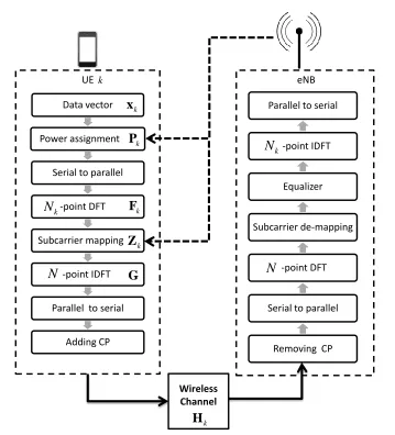
To enhance the power efficiency of UEs, LTE uses single carrier frequency division multiple access (SC-FDMA) in the uplink, while orthogonal frequency division multiple access (OFDMA) is used for the downlink. SC-FDMA has a lower peak-to-average power ratio (PAPR) when compared to OFDMA. The low PAPR advantage allows the power

(22)

amplifier at the transmitter to operate close to the saturation point which improves its effi-ciency. However, the lower PAPR feature of SC-FDMA requires contiguous allocation of the resource blocks (RBs) [9].

In this chapter, power-efficient schedulers for LTE uplink systems are proposed. The proposed schedulers are able to minimize the total instantaneous transmission power from all users while maintaining the LTE uplink physical layer constraints and the QoS require-ments. It is noteworthy that minimizing the total instantaneous transmission power can lead to minimizing the average transmission power specially in burst transmission.

The rest of the chapter is organized as follows. Section 2.2 presents the related work. Section 2.3 presents the system model. The system constraints and the objective of the work are presented in Section 2.4. The optimal and iterative formulations of the proposed scheduler are described in Sections 2.5 and 2.6, respectively. In Section 2.7 the PF scheduler is discussed. Intra-user scheduling is described in Section 2.8. Simulation results are presented in Section 2.9, and Section 2.10 concludes the chapter.

2.2 Related Work

The resource allocation problem for OFDMA systems has been widely investigated in the literature [11, 12]. As each RB cannot be assigned to more than one user, the resource allocation is a combinatorial optimization problem [11], which cannot be solved in polyno-mial time. Many studies have solved the allocation problem by using the convex relaxation method [11, 12]. The relaxation replaces the binary variables by continuous variables in the interval [0,1], then Lagrange multipliers are derived to solve the resource allocation. However, due to the contiguity constraint in SC-FDMA, the resource allocation methods that are applied to OFDMA are not directly applicable to the LTE uplink [13]. More details about the convex relaxation method are discussed in Section 2.4.

(23)

problem which is NP-hard. Consequently, low-complexity algorithms based on message-passing paradigm are proposed to solve the allocation problem in polynomial time. An-other sum-rate maximization scheduler that considers multiuser scheduling with transmit antenna selection is investigated in [15]. Based on local ratio test approach, suboptimal polynomial-time algorithms are proposed to solve the allocation problem. A scheduling approach based on a genetic algorithm is presented in [16] to solve the sum-rate maximiza-tion problem in LTE uplink systems. Nevertheless, sum-utility maximizamaximiza-tion problems usually lead to transmitting data using the maximum allowable transmission power, which often lowers the transmitter power efficiency [18].

A general packet scheduling scheme for LTE uplink is considered in [17]. The prob-lem is proven to be MAX SNP-hard. Consequently, two approximation algorithms for the scheduling problem are proposed to reduce complexity. The algorithms are evaluated for a specific scenario that incorporates the queue length and channel quality information. Leeet al. [19] investigated the proportional fair (PF) scheduler for the LTE uplink. The schedul-ing problem is proven to be an NP-hard because of the contiguity constraint. Heuristic algorithms were proposed and compared in terms of system throughput and fairness.

(24)

2.3 System Model

This study considers an LTE uplink multiuser system in a single cell, whereK UEs com-municate with an evolved node-B (eNB). It is assumed that each user has a maximum of four bearers, or logical channels, associated with different QoS requirements, an assump-tion which is justified in Secassump-tion 2.3.1. The overall cell bandwidth is divided equally intoM

RBs, each of which contains 12 adjacent subcarriers. The bandwidth of an RB is 180 kHz. To facilitate the readability, Table 2.1 summarizes the notations frequently used throughout the chapter.

The contiguity constraint which is required by SC-FDMA can be modeled by con-structing a binary matrixRas follows. Each column inRrepresents a potential contiguous allocation, while each row represents an RB. The column indexcin the matrixRwith the sizeM ×1is denoted byrc. Therefore,Rcan be expressed as

R= [r1,r2, ...,rC]. (2.1)

whereCis the number of columns inR, which can be calculated for a system that hasM

RBs as [20]

C = 1

2M(M + 1). (2.2)

For example, a system with 3 RBs has anRthat is equal to

R=



  

1 0 0

0 1 0

0 0 1

1 0 1

1 1 1

0 1 1



  

. (2.3)

To better understand the meaning of allocating one column ofRto a user, consider that the columnr1 is allocated to user k. The first element in r1 is one, which indicates that RB number one is allocated to user k. The second and third elements in r₁ are zeros, which indicates that RB numbers two and three are not allocated to userk. As can be seen in (2.3),

(25)

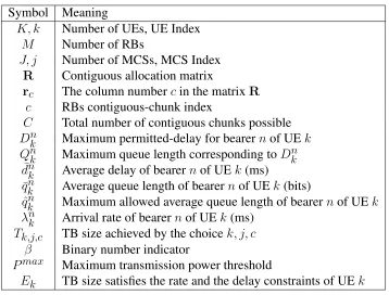
Table 2.1: Summary of the most significant notation used in this chapter. Symbol Meaning

K, k Number of UEs, UE Index

M Number of RBs

J, j Number of MCSs, MCS Index

R Contiguous allocation matrix

rc The column numbercin the matrixR c RBs contiguous-chunk index

C Total number of contiguous chunks possible

D_kn Maximum permitted-delay for bearernof UEk Qn_k Maximum queue length corresponding toD_kn

¯

dn_k Average delay of bearernof UEk(ms)

¯

qn_k Average queue length of bearernof UEk(bits)

ˆ

qn_k Maximum allowed average queue length of bearernof UEk λn_k Arrival rate of bearernof UEk(ms)

T_k,j,c TB size achieved by the choicek, j, c β Binary number indicator

Pmax Maximum transmission power threshold

E_k TB size satisfies the rate and the delay constraints of UEk

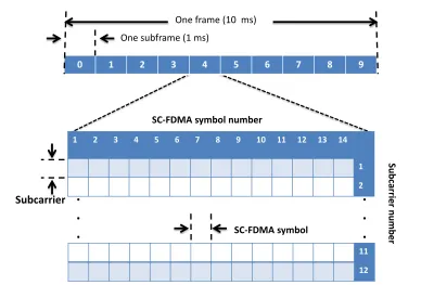
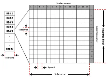
The LTE frame duration is 10 ms and it is composed of 10 LTE subframes. Each subframe has a duration of 1 ms, and represents a TTI [9]. When the normal cyclic prefix is used [9], each subframe consists of 14 SC-FDMA symbols, each with a duration of

66.67µs. Following the assumption used in [20], three symbols in each frame are assigned to uplink physical control signalling. The total number of data symbols in each RB per subframe is(14−3)×12 = 132. Fig. 2.1 shows the LTE subframe structure.

The LTE physical layer supports various modulation and coding schemes (MCSs). The MCS and the RBs that are assigned to a user determines the uplink transport block (TB) size. Suppose that the column vectorrc and the MCS numberj are assigned to user k, the TB size that userkcan transmit over a TTI is calculated as follows

T_k(j, c) =

132×ζ_j × krck (2.4)

whereζjis the MCS efficiency for the MCS numberjin terms of the number of useful bits

per symbol, krck is the the Hamming weight ofrc, which represents the number of RBs

(26)

1 2 3 4 5 6 7 8 9 10 11 12 13 14 1 2 3 4 5 6 7 8 9 10 11 12 Subframe 1 ms Symbol Subcarrier RB# 1 Subframe Symbol number Subc ar rie r numb er R e so u rc e b lock

Figure 2.1: The structure of the LTE subframe.

x.

The selection of MCS is determined such that the BLER is lower than the target BLER, which is 10% for LTE systems [9]. The BLER for each MCS depends on the effective received signal to noise ratio (SNR). A simple criterion for choosing appropriate MCSs is based on a set of SNR thresholds [9]. Given the effective received SNR for a user, the eNB selects the most spectrally efficient MCS that satisfies BLER < 10%. In practice, the BLER values are determined through a link-level simulator for all MCSs. Fig. 2.2 presents the simulation curves of the adopted MCSs in an LTE uplink over an additive white Gaussian noise (AWGN) channel [3]. Table 2.2 shows the modulation, code rate, spectral efficiency, and SNR thresholds for the MCSs [1]. The SNR thresholds can be obtained from Fig. 2.2.

The effective instantaneous received SNR for userk who is assigned column rc at

TTItis given by [20, 23]

γ_k[t] = 1

krck

X

m∈rc

α_k,m[t]P_k,m[t]

(27)

−10 −5 0 5 10 15 20 10−2

10−1 100

SNR [dB]

BLER

Figure 2.2: BLER-SNR curves for all Table 2.2 MSC, from Index 1 (leftmost) to index 15 (rightmost) [3].

whereP_k,m[t]is the transmission power of userk over the RB mduring the TTIt,

α_k,m[l] =h_k,m[t]

2

,h_k,m[t]is the channel gain of RBmat TTItseen by userk, andσ2

is the AWGN variance.

To reduce the signalling overhead, LTE specifies that when a user is assigned more than one RB, one power level should be transmitted over the assigned RBs [15]. In other wordsP_k,₁ = P_k,₂ = · · · = P_k,m.Therefore, the RB indexm can be dropped, and (2.5) can be written as

γ_k[t] = 1

krck2

X

m∈rc

α_k,m[t]P_k[t]

σ2 (2.6)

whereP_k[t] =krckPk,m[t]is the total transmission power of userkat TTIt. Using (2.6),

the required power to achieve an effective SNR ofγ_k[t]is

P_k[t] =γ_k[t] X m∈r_c

α_k,m[t]

!−1

krck2σ2 (2.7)

To recap, when user k transmits P_k over the RB chunk that is represented by rc,

(28)

Table 2.2: List of MCS indices [1]

Index j Modulation Coding Rate Spectral Efficiencyζ Effective SNR (dB)γk

0 — — 0 bits >−6.7536

1 QPSK 78/1024 0.15237 −6.7536 :−4.9620

2 QPSK 120/1024 0.2344 −4.9620 :−2.9601

3 QPSK 193/1024 0.3770 −2.9601 :−1.0135

4 QPSK 308/1024 0.6016 −1.0135 : +0.9638

5 QPSK 449/1024 0.8770 +0.9638 : +2.8801

6 QPSK 602/1024 1.1758 +2.8801 : +4.9185

7 16QAM 378/1024 1.4766 +4.9185 : +6.7005

8 16QAM 490/1024 1.9141 +6.7005 : +8.7198

9 16QAM 616/1024 2.4063 +8.7198 : +10.515

10 64QAM 466/1024 2.7305 +10.515 : +12.450

11 64QAM 567/1024 3.3223 +12.450 : +14.348

12 64QAM 666/1024 3.9023 +14.348 : +16.074

13 64QAM 772/1024 4.5234 +16.074 : +17.877

14 64QAM 873/1024 5.1152 +17.877 : +19.968

15 64QAM 948/1024 5.5547 >+19.968

through Table 2.2. Consequently, the TB size of userkcan be calculated from (2.4).

2.3.1 LTE QoS and Buffer Status Reports (BSRs)

LTE systems are designed to support a wide range of applications and services. In general, the user might run multiple applications simultaneously, each application requires differ-ent QoS. For example, a user can play real-time game while downloading a file using a file-transfer protocol. The eNB establishes multiple radio bearers per user to support mul-tiple QoS requirements as shown in Fig. 2.3. The LTE defines two main radio bearer categories [9]:

1. Bearers with guaranteed bit rate (GBR) are established for real-time applications such as voice and video, which require certain GBR to satisfy their QoS require-ments.

(29)

eNB UE

UL Data Flows

Radio Bearer Groups QCI

#1 QCI

#5 QCI

#6 QCI

#8 QCI

#9

Buffers Long- Format BSR

Figure 2.3: An example of four bearers established for a user.

(30)

2.3.2 Uplink Data Transmission Procedure

The sequence of uplink data transmission is shown in Fig. 2.4. The UE receives uplink traf-fic from upper layers. Data for multiple logical channels are queued in the RLC sub-layer buffers. Information about buffered data sizes is reported to the eNB over the physical up-link control channel using the BSR procedure. The scheduler in the eNB makes allocation decisions according to a specific scheduling policy. Based on the allocation decisions, the eNB sends allocation maps to the users over the physical downlink control channel. The user’s allocation map specifies the assigned RBs, power control entity and MCS [24]. The power control entity specifies the uplink transmission power for each user. The RBs chunk and MCS that is assigned to a user determine the uplink transport block TB size. However, how the TB is shared between users’ buffers is left to the user policy, which is discussed in Section 2.8.

In the UE media access control (MAC) sub-layer, a MAC protocol data units (PDU) is formed according to the received map allocation. The MAC PDU contains data from one or more RLC PDUs in addition to the MAC header. The MAC passes the MAC PDU to the physical layer (PHY), which adds the cyclic redundancy check (CRC) bits to the MAC PDU and then transmits the entire packet as a TB over the physical uplink shared channel to the eNB. The PHY responsibility is to deliver the TB with an error probability less than a targeted BLER.

2.3.3 Delay Analysis

As mentioned in Section 2.3.1, the BSR does not report explicit information about PDU delays, but reports the sizes of the queued data in the UE buffers. In this section, the PDU delay is mapped to the size of the queued data. The queue evolution during TTIt+ 1can be described as

(31)

RLC

MAC

PHY MAC

header 4 4 3 2 1 1

CRC

MAC

header 4 4 3 2 1 1

UE

1 1 1 1 2

2 3

3 3 4

4 4 4 4

1

i 

2

i 

3

i 

4

i 

eNB Allocation

Map BSR to eNB

CSI Scheduler RLC

PDUs

TB MAC PDU

(32)

LTE defines a packet delay budget (PDB) for each bearer, which defines an upper bound for the time that a packet may be delayed between the UE and the packet data network gateway. In LTE, the outage delay outage level should be less than 2% [9]

P(dn_k >Dˇn_k)<0.02 (2.9)

wheredn_k is the head of the line packet delay, andDˇ_knis the PDB. For high data traffic load, the following approximation is valid [25]

P(dn_k >Dˇn_k)≈e

−Dˇn

k/d¯nk

(2.10)

where d¯n_k is the average value of dn_k. Therefore, in the case of high data traffic load, controlling d¯n_k is approximately equivalent to controlling the delay violation probability

P(dn_k > Dˇn_k). The justification for the assumption of heavy data traffic is that most delay violations take place when the traffic load is heavy. By substituting (2.9) into (2.10), the required average delay for bearernof userkis given by

¯ dn_k <−

ˇ Dn_k

ln(0.02). (2.11)

This work focuses on the the air-interface delay between UEs and eNB. It is assumed that the air-interface delayD_kncontributes toδof the PDB as follows

Dn_k =δDˇn_k (2.12)

where0≤δ≤1. Using Little’s theorem [22], the average delay can be computed as

¯ dn_k = q¯

n k

λn_k (2.13)

whereq¯_kn is the average queue size. Substituting (2.13) and (2.12) into (2.11), the bearer air-interface delay can be controlled by controlling the average number of bits in the users’ queues

¯

(33)

ˆ

q_kn =− Q

n k

ln(0.02) (2.14b)

whereqˆ_knis the maximum allowable average queue length of bearernof userkthat satisfies the delay requirement, andQn_k =D_kn×λn_k is the average queue length that corresponds to the air-interface delayDn_k.

It is worth noting that the size of the data buffers is assumed to be greater than the PDBs for all bearers. If the size of a buffer is less than the PDB, the PDB is assumed to be the maximum buffer size for that bearer.

It is assumed that the eNB knows, or at least can estimate, the average arrival rates for all bearers and users. One way to estimate the average arrival rates is reported in [26]. Suppose that the scheduler successfully maintains the delay requirements of buffer number

nof userksuch thatq_kn ≤qˆn_k, the average arrival rateλn_k is equal to the long-term average of the service rateT_kn.

2.4 System Constraints and Objective

The resource allocation in LTE uplink requires the following constraints to maintain the physical layer restrictions and the QoS requirements:

1. Exclusivity constraint: for every TTI, a single RB is allocated to no more than one user.

2. Contiguity constraint: SC-FDMA restricts the RB allocations to be contiguous. Each column in the matrix R represents a contiguous RB allocation. The conti-guity constraint can be maintained by assigning one column from the matrixRto each user.

3. Power constraint: the LTE standard specifiesPmax as the maximum transmission power threshold that the user cannot exceed.

4. Rate constraint: minimum bit rate for the GBR bearers must be maintained.

5. Delay constraint: NGBR bearers subject to PDB. As discussed in Section 2.3.3, the delay constraint can be maintained by controlling the average queue length.

(34)

question: how should the available resources, in terms of RBs and transmission power, be assigned to the users so that the total transmission power is minimized without violating the users’ QoS requirements? Without loss of generality, a finite time horizon of length

F TTIs is chosen. It is assumed that the current time is t and the observation interval is

[t, t+F]. DenoteW(x[t], L)as a sliding-average window of lengthLfor variablex

W(x[t], L) = 1 L

t+L X

l=t

x[l], (2.15)

and denoteP_k,j,c[l]as the transmission power required to achieved the target BLER when userk transmits using the MCS number j over the RB allocation numbercat TTIl. The resource allocation problem can be written as

min t+F

X

l=t K X

k=1

J X

j=1

C X

c=1

P_k,j,c[l]β_k,j,c[l] (2.16a)

subject to

K \

k=1

rcβk,j,c[l] =∅, ∀l, j, c (2.16b)

P_k,j,c[l]≤Pmax,∀l, k, j, c (2.16c)

W(T_kn[t], F)≥r_kn (2.16d)

W(qn_k[t], F)≤Dmarg ×qˆn_k (2.16e) whereβ_k,j,c[l]is a binary number indicator that is equal to 1 if and only if the MCS num-ber j and the column rc are selected for user k at TTI l, J is the total number of MCSs, Dmarg ∈(0,1)is a margin used to maintain the delay less than the maximum in (2.14), and rn_k is GBR of the bearer numbern of userk. Note that the exclusivity constraint is main-tained by (2.16b), where the summation over crestricts the users to only contiguous RB allocations and maintains the contiguity constraint. The power, rate, and delay constraints are maintained by (2.16c), (2.16d), (2.16e), respectively.

(35)

exist to solve MDPs, they suffer from the curse-of-dimensionality problem [27], where the number of states grows vastly with the numbers of both users and bearers. Conse-quently, formulating and solving constrained MDPs is non-trivial as it deals with an ex-tremely large number of transition probabilities. Therefore, approximated solutions are often provided [27]. Moreover, a comprehensive knowledge of the users’ channel gains and arrival processes may be required to solve the MDP. A similar problem in OFDM sys-tems is investigated in [12] by relying on stochastic convex optimization. For each TTI, the allocation depends on the instantaneous channel gains and Lagrange multipliers. The mul-tipliers are associated with the QoS requirements and are estimated online using stochastic approximation tools. However, many approximations are used while turning this problem into a stochastic convex optimization. First, Shannon’s capacity formula is used (contin-uous rate adaptation) instead of a practical discrete set of MCSs. Second, the exclusivity constraint is relaxed. The relaxation replaces the binary indicators by contentious variables belong to the interval[0,1]. In OFDMA each binary number refers to a single RB or sub-carrier. Having a fraction of a subcarrier translates into time sharing between users for the subcarrier which creates a form of time-division multiple access. However, in SC-FDMA, the allocated RBs for a particular user should be adjacent, and sharing chunks of RBs over time is not applicable because the contiguous allocation is not guaranteed [13]. Third, it is observed that, optimum values of the multipliers can never be found. Therefore stochastic approximation is used to estimate the multiplier values.

An alternative approach to solve (2.16) is to design a non-causal optimal offline scheduler, which gives a guideline to design and evaluate online suboptimal schedulers. The offline optimal scheduler requires a prior knowledge of both arrival data units and channel state information for{t, t+ 1, ..., t+F}at TTIt. Therefore, the problem turns into a discrete time deterministic control process, which can be solved, for example, by binary integer programming. Nevertheless, the search space of this formulation is extremely large and can be calculated as follows. For one TTI, for userk, there are 1₂M(M + 1)possible allocations in the frequency domain as shown in (2.2). For each possible allocation, J

MCSs exist. Therefore, the total number of choices possible for userkis J₂M(M+ 1). For theK users, the search space is

J

2M(M + 1)

K

(36)

TTIs is

J

2 M(M + 1)

KF

. (2.17)

For example, assume a system with the following parameters: M = 6RBs,J = 15MCSs,

K = 4andF = 10TTIs. The search space size is8.5590×1099.

In the following sections, a computationally feasible version of the scheduling prob-lem is presented.

2.5 BIP Formulation

To simplify the scheduler and to avoid the computationally-excessive optimization in (2.16), a formulation of the optimization problem for a single time slot (F = 1) is presented here. The exclusivity, contiguity, and power constraints must be satisfied for each TTI because they are related to the physical system. However, the rate and delay constraints are based on averages, which means they are soft and it is not necessary to satisfy them every TTI. In other words, the rate and/or delay might not meet their QoS requirements at certain times, but on average over a long time interval, the QoS requirements are met. Allowing the rate and delay constraints to be soft avoids infeasible instantaneous solutions. Such solutions appear when the instantaneous required data transmission rate is greater than the instant channel capacity. However, it is assumed that, in the long term, the channel capacity can provide the required QoS. In cases where the QoS requirements are greater than the avail-able channel capacity, scheduling becomes infeasible, and dropping users may be the only feasible solution [12]. An admission control procedure is responsible for deciding which user should be dropped or admitted in such cases. This study does not consider admission control procedures, and it is assumed that the average channel capacity can manage the required QoS.

(37)

−6−5 0 5 10 15 20 0

1 2 3 4 5 6

SNR (dB)

Spectral efficiency (bit/s/Hz)

MCS

MCS # 13

MCS # 9 MCS # 7

MCS # 11

Figure 2.5: Spectral efficiency versus SNR for the MCS that are shown in Table 2.2.

Table 2.2 and their corresponding effective SNRs. From (2.7), the transmission power de-creases as a function of the effective SNR for a specific RB chunk allocation, which implies that the transmission power is logarithmically related to the spectral efficiency of the trans-mission. For example, transmitting four symbols using MCS number four is equivalent to transmitting one symbol using MCS number nine. Although, the former transmission requires additional four time slots, it consumes only 43% of the later transmission power consumption. Therefore, splitting the data and transmitting lower data rates over more sub-frames eventually lowers the total transmit power. However, the data rates should maintain the users’ QoS requirements.

Modulation and coding schemes are less power-efficient at higher transmission rates [28]. Therefore, the scheduler is designed to judiciously transmit the minimum number of bits that softly satisfies the rate and the delay constraints at each TTI. Then by optimal power allocation, optimal chunk of RBs is assigned to each user. DefineB_kn as the mini-mum number of transmit bits that satisfy both the rate and the delay constraints to bearer

(38)

constraints is

E_k =

4

X

n=1

B_kn.

As the rate and the delay constraints are converted to soft constraints, the minimum-cost solution is a trivial one, i.e., no power is consumed if no data is transmitted. To address this issue, an extra weightρ_k,j,cis defined and added to the applied power cost as follows

ρ_k,j,c = log(E_k)−log(T_k,j,c/E_kGBR), T_k,j,c >0, (2.18)

where the T_k,j,c are the TB achieved using MCS j over the RB allocation numberc, and

E_kGBR is the number of bits that satisfies all the GBR bearers of userk

E_kGBR = X

n∈N_kGBR

B_kn, (2.19)

whereN_kGBRis a set contains the index of the GBR bearers that belongs to userk.

The weightsρ_k,j,c measure how close theE_kare to the actual transmitted TBT_k,j,c. To better illustrate extra weights, consider the demonstration shown in Fig. 2.6. Two main interesting characteristics can be observed. First, users with higher E_kGBR values have higher weights, which gives them a higher priority through the scheduling. Second, as the number of bits transmitted increases, weight values drop rapidly when T_k,j,c < E_kGBR, but slightly whenT_k,j,c > E_kGBR. The second characteristic implies that satisfying GBR requirements for all users are more important than that for NGBR requirements.

In this context, for single TTI, (2.16) is expressed as (time index is omitted for sim-plicity)

min K X

k=1

J X

j=1

C X

c=1

ρ_k,j,c+P_k,j,c

β_k,j,c (2.20a)

subject to

T_k,j,c ≤E_k (2.20b)

(39)

0 0.1 0.2 0.3 0.4 0.5 0.6 0.7 0.8 0.9 1 1.5

2 2.5 3 3.5 4 4.5

Tk,j,c/Ek

ρk

,j

,c

B_kGBR/E_k=.25 B_kGBR/E_k=.5 B_kGBR/E_k=.75

Figure 2.6: Extra weight demonstration forE_k = 200bits.

2.5.1 Binary Integer Programming

Thebintprogoptimization package from MATLAB is used to solve the non-convex prob-lem. The general form of a BIP optimization can be presented as

mincTx (2.21a)

subject to

Ax≤b, Aeqx=beq, (2.21b)

where the vector crepresents the weights ρ_k,j,c plus the transmission power costsP_k,j,c, and the binary decision vectorxminimizes the objective function and represents the term

β_k,j,c in (2.20a). Constraints (2.20b), (2.20c) are maintained by linear inequality and equality constraints,Ax≤ b,Aeqx=beq, respectively, whereA,Aeq are matrices

con-taining the coefficients of the inequality and equality constraints, andb,beqare vectors that

(40)

allo-cation. For each feasible contiguous allocation,J different MCSs are possible, the matrix which contains all feasible contiguous allocations for all MCSs is defined as

A_k = [R,R, . . . ,R

| {z } J

]. (2.22)

Each column in (2.22) is associated with a potential transmit power cost calculated from

P_k,j,c. The power constraint is maintained by deleting columns with potential transmission power greater thanPmax. Define the matrix Ath_k which has all columns inA_k less than or equal toPmax. Define matrixA which concatenates all matricesAth_k for all users as follows:

A=hAth₁ ,Ath₂ , . . .Ath_Ki, (2.23) where each row inA represents a single RB, to ensure the exclusivity constraint, and the vector b = 1_M, where 1_M is a vector of M ones. The equality constraints maintain a unique selection from all feasible allocations for all data sizes per user, and therefore

J X j=1 C_k X c=1

β_k,j,c= 1,∀k.

The equality constraints are expressed as follows

Aeq =        1T A th 1

· · · 0T

A th K .. . . .. ... 0T A th 1

· · · 1T

A th K        (2.24) where A th k

is the number of columns inA th

k which denotes the number of potential

al-location choices for user k, and 1T_x,0T_x are row vectors of length x of ones and zeros, respectively. The vector beq is defined as beq = 1K to guarantee that only one of the

(41)

2.5.2 Complexity of BIP

Consider the worst case scenario, where all columns inA0_k,∀kare less or equal toPmax. The search space of BIP formulation is similar to the search space of (2.17) for a single TTI (F = 1)

1

2J M(M + 1)

K

. (2.25)

For example, assume a system with the following parameters: M = 6 RBs, J = 15 MCSs, and K = 4. The BIP worst case search space size is 9.8456 ×109. Thus, the approach as formulated is still computationally expensive. Therefore, low-complexity algorithms are needed to solved the resource allocation problem.

2.6 Iterative Algorithm

In this section, an iterative algorithm is proposed to solve the BIP with much less compu-tational complexity. The algorithm belongs to the greedy algorithm family. The objective is to minimize the summation of the total users’ costs by assigning RBs to the users it-eratively. In each iteration, a single RB is assigned to a user who can achieve maximum reduction in the cost function. Therefore, the algorithm needsM iterations to assign all the RBs to users. For each iteration, the algorithm finds the best RB for each user. The best RB of userk is defined as the RB that has the highest instantaneous channel gain (α_k,m) and satisfies the contiguous allocation of user k. Then, the change in the user’s cost value be-fore and after assigning the best RB is calculated for each user. As the algorithm is greedy, the user who has the maximum positive change in the user’s cost function is granted the allocation. The pseudo-code in Table 2.3 describes the algorithm. The proposed algorithm consists of four main steps as follows:

Lines 1-7: find the minimum rate (E_k) for each userk that satisfies the rate and the delay constraints. In addition, in this step the following parameters are initialized: the set of users index K, the set of non-assigned RBs M, the set of RBs that assigned to users

(42)

Lines 8-14: find the best feasible RB F_k for each user k. Users, who have been assigned one or more RB, are limited to their neighboring RBs (line: 11). Therefore, two RBs are feasible at most to any user who has been assigned one or more RBs. For example, suppose that user k has been assigned the RB numbers {4,5,6}. Therefore, the feasible RBs to userkare3and7if they are not assigned to any user. However, users who have not yet been assigned RBs can select any RB of the non-assigned RBs setM(line: 13). In the case that a user has more than one feasible RB, the algorithm selects the RB that has the maximum instantaneous channel gain.

Lines 15-21: after finding the best feasible RB to each user, the users’ cost values of the new potential allocation sets are computed Ψ∗_k,∀k ∈ K. Then, the potential cost reduction∆Ψ_k for each user is computed, where∆Ψ_kis the difference between the actual cost valueΨ_k and the potential cost valueΨ∗_k. If all users do not benefit (reduce their cost values) from the new potential allocation sets, the algorithm stops (lines 19 and 20). The

COST(M_k, E_k)function finds the total costs, i.e. ρ_k,j,c+P_k,j,c, associated with assigning the set of RBsM_kto userk. In case ofM_k =∅, the total cost isCOST(∅, E_k) = log(E_k), as illustrated in line 5.

Lines 22-26:determine the winning user who achieved the maximum cost-reduction

∆Ψ∗_k (lines 22). Then the algorithm assigns RB F_k∗ to the winning user (lines 24), and updates the set of non-assigned RBs (lines 25).

2.6.1 Complexity of the Iterative Algorithm

For each major iteration (lines 8-27), an RB is allocated, and therefore, the maximum number of major iterations isM. The first major iteration for each user requires at most

(43)

Table 2.3: Iterative allocation

1: M={1,2, . . . , M} 2: K={1,2, . . . , K} 3: fork∈ Kdo

4: findEk 5: Ψk= log(Ek) 6: Mk=∅

7: end for

8: while|M 6=∅|do

9: fork∈ Kdo

10: ifM_k6=∅then

11: F_k= arg max

m∈{min(Mk)−1,max(Mk)+1}∩M

{αk,m}

12: else

13: F_k= arg max

m∈M

{αk,m}

14: end if

15: M∗_k=Mk∪ Fk 16: Ψ∗_k=COST(M∗_k, Ek)

17: ∆Ψk= Ψk−Ψ∗k

18: end for

19: ifΨ∗_k<0, ∀k∈ Kthen

20: exit

21: else

22: k∗ = arg max

k

{∆Ψk}

23: Ψk= Ψ∗_k

24: M∗_k=M_k∪ F_k

25: M∗ ₌_{M \ F}

k

26: end if

(44)

the maximum number of RBs in LTE system is 100 RBs. Thus, the complexity of such scenario is in the order of10,000iterations.

2.7 Proportional Fair Scheduler

The PF scheduler has been widely investigated in the literature. The objective of the PF scheduler is maximizing the total throughput of the system while maintaining level of fair-ness between users. Leeet al. [19] investigated the PF scheduler for SC-FDMA systems. The scheduling problem is known to be an NP-hard.

To determine the power efficiency of the proposed algorithms, the PF scheduler is used as the baseline scheme for comparison. The PF scheduler of [19] have been modified to cope with our system model. The objective function at TTItcan be expressed as

max K X

k=1

J X

j=1

C_k X

c=1

ω_k[t]×T_k,j,c[t], (2.26a)

subject to

(2.16b), (2.16c) (2.26b) where ω_k[t] is a scheduling weight assigned to userk at TTI t. The scheduling weights depend on transmission history for users as follows

ω_k[t] = 1

W(T_k[t−1], L_{P F}) (2.27)

whereW(T_k[t −1], L_{P F}) is a sliding-average window defined in (2.15) of lengthL_{P F}. Users who have low historical average data rates are assigned higher weights than those who have high historical average data rates, which increases their chances of obtaining more RBs during the scheduling.

(45)

Table 2.4: Intra-user scheduling for userk 1: E_kGBR= P

n∈NGBR k

B_kn

2: E_kN GBR= P n /∈NGBR

k

B_kn

3: ifE_kGBR< Tkthen 4: T_kn=B_kn, ∀n∈ NGBR

k 5: Tn

k = (Tk−EkGBR)×(Bkn/EkN GBR), ∀n /∈ NkGBR 6: else

7: T_kn=Tk×(Bkn/EkGBR), ∀n∈ NkGBR 8: Tn

k = 0, ∀n /∈ NkGBR

9: end if

2.8 Intra-User Scheduling

In all the scheduling schemes discussed above, the scheduler output is the setT_k, ∀k = 1,2, ..K, which indicates the TB size for each user. It is assumed that UEs share their TBs between their bearers as follows:

1. GBR bearers should be satisfied before NGBR bearers.

2. Within the same radio bearer category (GBR or NGBR), the allocated resources are distributed proportionally toB_kn. In case of PF scheduler, B_kn are replaced by the queues length of bearern.

The pseudo-code in Table 2.4 describes the intra-user scheduling, whereT_kndenotes the portion ofT_k allocated to bearernof userk.

2.9 Numerical Results

The simulation default parameters are shown in Table 2.5. The channel is modeled as a quasi-static frequency-flat Rayleigh fading channel. The channel gain is assumed to be constant over each RB bandwidth, but change independently over consecutive RBs. More-over, it is assumed that users experience independent fading. For a Rayleigh fading chan-nel, the distribution of the instantaneous received channel gain αfollows the exponential distribution [29]

p α_k,m= 1 α_ke

−αk,m

(46)

Table 2.5: Simulation default parameters

Parameter Value Parameter Value Coherence time 1 ms M 10

UE # 2 Iteration # 1e4

BW 15 kHz Cells interference Avoidance

δ 1 Dmarg 0.9

Pmax 23 dBm L_{P F} 50

Channel fading Rayleigh L 8 Target BLER 10 % σ2 1

Table 2.6: Users’ data profile

Index Type λn_k(Kbps) Dn_k(ms) Qn_k(bits) qˆ_kn rn_k(Kbps)

B1 NGBR 100 20 2000 511 0

B2 GBR - - - 50

B3 NGBR 75 20 1500 383 0

B4 GBR - - - - 30

whereα_k is the expected value ofα_k,mand denotes the average channel gain (ACG). Table 2.6 presents bearers profiles. NGBR bearers serve non real-time applications. It is assumed that the data arrivals for non real-time traffic follow a Poisson distribution as it has been used in related works [22, 26, 30].

(47)

2.9.1 Experiment 1: Two Users with Identical Conditions

In this experiment, a two-user scenario with an identical traffic load and channel profile is considered. Because the users experience identical conditions in terms of channel and traffic load, it is sufficient to show results for only one user. Each user is assumed to have two bearers, namelyB1andB2.

Fig. 2.7 compares the transmit power for the three schedulers. The BIP consumes slightly less power than the iterative scheduler, and both of them consume approximately 43% less power than the PF scheduler. To better visualize the efficiency of the schedulers, consider the following scenario: users transmit data until the total power consumption reaches 80 Watt. Note that 80 Watt is equivalent to transmitting at the maximum power threshold (200 mW) for 400 TTIs. Fig. 2.8 shows that the BIP and iterative schedulers prolong the battery life considerably compared with the PF scheduler for the same QoS requirements.

Fig. 2.9 compares the average queue length of the two bearers for the three sched-ulers. All the schedulers succeed in maintaining average queue lengths of the NGBR data less than the threshold. As the intra-scheduling serves the GBR bearers before the NGBR bearers, the queue lengths of the GBR bearers are shorter than the queue lengths of the NGBR for all schedulers. The PF scheduler tends to transmit aggressively, i.e., the max-imum achievable data rate. Therefore, the average queue lengths of the PF scheduler are lower than those for the other two schedulers. The queue lengths of the BIP scheduler are slightly shorter than the queue lengths of the iterative scheduler.

(48)

10 12 14 16 18 20 22 24 26 28 30 0.04

0.06 0.08 0.1 0.12 0.14 0.16

Average channel gain

Average transmit power per user

Iterative BIP PF

Figure 2.7: Experiment 1: Average transmitted power per user per TTI (Watt).

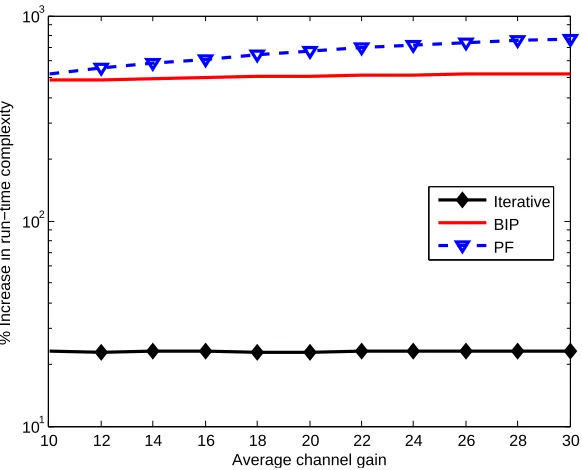
are compared in Fig. 2.12. The MATLAB functionsticandtocwere used to measure the running time. As expected, the running time of the iterative scheduler is significantly less than that for BIP and PF. Increasing ACG has no effect on the iterative and BIP running times. However, it is directly proportional to the PF time complexity. As ACG increases, more MCSs are considered in each RB chunks, which increases the size of the search space evolved in each iteration.

2.9.2 Experiment 2: Two Users with Identical Conditions but

Different ACG

TTo illustrate the behavior of the PF scheduler, two users with different ACGs are consid-ered. The ACG of user one is fixed to 10, whereas the ACG for user two varies from 10 to 30 (10 dB to 14.8 dB). The transmission power for user one and user two are shown in Fig. 2.13 and Fig. 2.14, respectively. Increasing the ACG of user two reduces transmit power consumption. However, this increase has no effect on the power consumption of user one who experiences a constant average channel fading.

(49)

10 12 14 16 18 20 22 24 26 28 30 1

1.2 1.4 1.6 1.8 2 2.2 2.4 2.6 2.8 3

Normalized battery life

Iterative BIP PF

Figure 2.8: Experiment 1: Battery life comparison.

three schedulers maintain average queue lengths of the NGBR bearers less than the maxi-mum allowed average queue length (q¯_kn <qˆ_kn). As user two ACG increases, shorter queue lengths are observed. However, user one queue length remains unchanged. In summary, the proposed schedulers isolate the users from each other. Users who experience good channel conditions consume less power than users who experience severe fading conditions. Fig. 2.16 shows that the transmission rates are equal to the data arrival rates, which implies that all the data arrived has been transmitted.